Article

The Retrieval of Forest and Grass Fractional Vegetation Coverage in Mountain Regions Based on Spatio-Temporal Transfer Learning

1
Aerospace Information Research Institute, Chinese Academy of Sciences, Beijing 100094, China
2
University of Chinese Academy of Sciences, Beijing 100049, China
*
Author to whom correspondence should be addressed.
Remote Sens. 2023, 15(19), 4857; https://doi.org/10.3390/rs15194857
Submission received: 14 August 2023 / Revised: 1 October 2023 / Accepted: 2 October 2023 / Published: 7 October 2023

Abstract

:
The vegetation cover of forests and grasslands in mountain regions plays a crucial role in regulating climate at both regional and global scales. Thus, it is necessary to develop accurate methods for estimating and monitoring fractional vegetation cover (FVC) in mountain areas. However, the complex topographic and climate factors pose significant challenges to accurately estimating the FVC of mountain forests and grassland. Existing remote sensing products, FVC retrieval methods, and FVC samples may fail to meet the required accuracy standards. In this study, we propose a method based on spatio-temporal transfer learning for the retrieval of FVC in mountain forests and grasslands, using the mountain region of Huzhu County, Qinghai Province, as the study area. The method combines simulated FVC samples, Sentinel-2 images, and mountain topographic factor data to pre-train LSTM and 1DCNN models and subsequently transfer the models to HJ-2A/B remote sensing images. The results of the study indicated the following: (1) The FVC samples generated by the proposed method (R2 = 0.7536, RMSE = 0.0596) are more accurate than those generated by the dichotomy method (R2 = 0.4997, RMSE = 0.1060) based on validation with ground truth data. (2) The LSTM model performed better than the 1DCNN model: the average R2 of the two models was 0.9275 and 0.8955; the average RMSE was 0.0653 and 0.0735. (3) Topographic features have a significant impact on FVC retrieval results, particularly in relatively high-altitude mountain regions (DEM > 3000 m) or non-growing seasons (May and October). Therefore, the proposed method has better potential in FVC fine spatio-temporal retrieval of high-resolution mountainous remote sensing images.

1. Introduction

Mountains cover approximately 30% of the Earth’s surface. Forest and grassland, as important components of mountain ecosystems, provide critical resources for human survival and development and prevent natural disasters such as landslides and debris flows. Additionally, they play a crucial role in maintaining regional and global ecological balance and regulating climate change [1,2,3]. Thus, monitoring and protecting forest and grass vegetation cover in mountain areas is essential. Fractional Vegetation Cove (FVC) is defined as a vertical projection of the areal proportion of a landscape occupied by green vegetation [4], which can characterize the vegetation coverage and is often used to quantify the dynamic changes of vegetation on a regional or global scale [5]. With global climate change and the intensification of human activities, forest and grass vegetation coverage in the mountains, particularly plateau areas with relatively fragile ecological environments, has been destroyed. Therefore, the dynamic monitoring and protection of FVC in mountain areas is a critical and long-term research topic that requires sustained attention.
Remote sensing Earth observation provides key technology for large-scale, multi-temporal FVC retrieval and monitoring at regional and global scales, and it is also available in mountain areas. At present, remote sensing-based FVC products, including GEOV2 FVC [6], GEOV3 FVC [7], and GLASS FVC [8], have been extensively utilized for global FVC monitoring and have achieved positive results [9,10,11]. However, these products typically have coarse spatial resolutions ranging from hundreds of meters to kilometers [12], and higher-resolution FVC products are relatively scarce. The high diversity of forest and grass types, frequent cloud cover, and rugged topography in mountain areas make it challenging for existing FVC products to capture the fine-scale heterogeneity of mountain topography, which results in increased uncertainties in FVC estimation [13,14,15,16]. Therefore, to ensure the accuracy of FVC estimation in mountain regions, it is necessary to adopt higher-resolution remote sensing images and consider topographic factors [17,18].
The methods of FVC estimation include a physically based model, linear spectral mixture models (LSMA) based on vegetation index (VI), and machine learning (ML). The physical model is mainly to establish a look-up table (LUT) based on PROSAIL [19], a vegetation radiative transfer (RT) model, to estimate the FVC. However, physical methods require more input parameters and prior knowledge of the vegetation canopy. The complex topography and lack of prior knowledge of vegetation in mountain areas increase the difficulty of FVC estimation. The LSMA model [20,21], known as the pixel dichotomy model, is the simplest FVC estimation method and is commonly used in medium-resolution or high-resolution images. Nevertheless, the normalized difference vegetation index (NDVI), as the variable of the pixel dichotomy model, usually exhibits the phenomena of “saturation” in areas with dense vegetation canopy cover in mountain areas, resulting in an overestimation of FVC [22,23]. The ML [24] method establishes an FVC estimation model by training a large number of high-precision samples composed of FVC values and spectral reflectance or VI. This method has been widely applied due to its excellent ability to handle nonlinear problems and reliable results. Typically, high-precision FVC samples come from drone images in the field or satellite images with fine pixel scale (resolution ≤ 1 m) [25,26]. However, mountain areas are easily affected by cloud and fog cover, and the topographic effect causes huge differences in slope vegetation spectral reflectance, resulting in scarce and difficult-to-obtain high-precision FVC samples. In addition, traditional ML algorithms are only applicable to vegetation bands or VIs in specific areas, and for images with different resolutions and temporal phases, the dataset and training need to be reconstructed, resulting in poor transferability.
Transfer learning (TL) is used to improve a learner from one domain by transferring information from a related domain [27,28,29,30]. In the study of vegetation quantitative retrieval, TL achieves model transfer by applying a pre-trained model from high-precision samples in one region to a new region or new remote sensing data source. Research has reported that the TL model is more robust than traditional ML models in crop FVC and yield estimation [31,32,33]. Astola [34] used the DNN-based TL model to predict structure variables of several forests, revealing that TL can solve the problem of model performance degradation caused by insufficient reference data in the field. TL can be realized by pre-training simulated samples, while high-precision samples are lacking. The RT mode can provide sufficient training samples for the TL model by generating simulated vegetation parameters. Yu [35] estimated the FVC of winter wheat in Sentinel-2 images (RMSE = 0.06) by using the LSTM model pre-trained on the simulated FVC samples generated with PROSAIL.
The TL model trained with simulated FVC holds great potential in predicting spatio-temporal variations of FVC in complex high-altitude mountain regions. Estimating FVC in mountain regions requires the consideration of not only vegetation spectrum and VIs but also topographic gradients, incorporating slope and aspect. At present, the RT models employed in generating vegetation parameter samples seldom account for the effects of topographic undulation, leading to limited sample accuracy in complex mountain regions. The accuracy of these samples can also impact the model’s precision in predicting FVC spatio-temporal variations.
Aiming at the current problem of lack of FVC training samples in mountain areas and difficulty in obtaining them, this paper proposed a method for estimating forest and grassland FVC distribution based on spatio-temporal TL in mountain areas, considering topographic factors. The flowchart of the proposed approach is shown in Figure 1: (1) We established a sample classification system based on the characteristics of mountain areas, considering the type of surface features and the characteristics of altitude gradients. (2) Based on the high-resolution remote sensing data, we established the FVC sample by using the PROSAIL model. (3) We Used FVC samples to train 1DCNN and LSTM models. (4) We fine-tuned the pre-trained model and obtained the distribution of FVC.

2. Materials and Methods

2.1. Study Area

The study area (Figure 2) is located in the mountain area (101°48′~102°42′E, 36°29′~37°11′N) of Huzhu Tu Autonomous County, Qinghai Province, China. The study area covers an area of 3321 km2, with an elevation ranging from 2100 m to 4360 m. The southwest part of Huzhu County is dominated by a basin with crops and urban, while the northeast part is a mountain area covered by grassland and forest. This region belongs to the continental cold temperate climate, the average annual temperature is 5.8 °C, the average annual precipitation is 447 mm, and the mountain vegetation in this region shows obvious seasonal changes.

2.2. Data Sources

2.2.1. Remote Sensing Image Data and Preprocessing

In the study, the multispectral time series remote sensing images of Sentinel-2 with 10 m resolution and HJ-2A/B with 16 m resolution are selected. Sentinel-2 imagery was utilized to construct a TL sample dataset in the study area. To reflect the seasonal variation of FVC in the study area, Sentinel-2 data with cloud cover of less than 20% from May to October during 2019–2022 were selected. The Sentinel-2 data was sourced from the Copernicus Open Access Hub, ESA (https://scihub.copernicus.eu/dhus/#/home, accessed on 1 October 2023). HJ-2A/B data served as the target images for FVC retrieval and were obtained from the China Centre for Resources Data and Application (https://data.cresda.cn/#/2dMap, accessed on 1 October 2023). The digital Satellite elevation model (DEM) of the study area was obtained from the Shuttle Radar Topography Mission (SRTM) with a 30 m spatial resolution and was used to calculate slope and aspect.
Preprocessing operations, including radiometric calibration, atmospheric correction, and geometric correction, were conducted to obtain a reflectance dataset of satellite images. We used the monthly maximum synthesis method [36] to remove cloud shadow interference and obtained 24 phases of Sentinel-2 and 6 phases of HJ-2A/B cloud-free time series images. The DEM was resampled to the same resolution as the Sentinel-2 and HJ-2A/B images, respectively, and topographic slope and aspect were calculated.

2.2.2. Site FVC

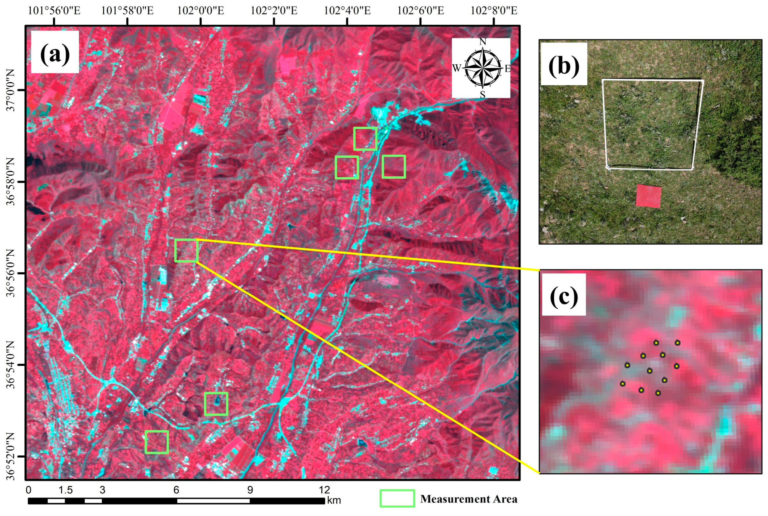
Site FVC for validation was taken in the mountain vegetation coverage area of Huzhu County from 10 to 12 September 2022. At all measurement points, FVC was recorded by analyzing digital photographs and visual estimation, and a total of 43 ground measurement points were obtained. The FVC measurement value can be obtained by calculating the percentage of green pixels in the white rectangle frame in the digital photographs taken on the spot (Figure 3b) to all pixels in the white rectangle. The green pixels and non-green pixels in digital photographs are extracted with Marcial-Pablo’s method [37], and the FVC measurement value calculated is as follows:
F V C m e a s u r e d = p i x e l g r e e n p i x e l t o t a l
where  F V C m e a s u r e d  is the measured FVC, and  p i x e l g r e e n  and  p i x e l t o t a l  are the green pixels and the total number of pixels in the digital photograph, respectively.

2.2.3. Vegetation Cover Classification

In this study, the Global Land Cover with Fine Classification System at 30 m in 2020 [38] was utilized as a reference dataset for land cover classification. The experimental area includes various land cover types, such as grassland, forest, cropland, water bodies, and urban areas, as illustrated in Figure 2c. For this study, we focused on two types of vegetation, namely forest and grassland. Based on the distribution of vegetation at different elevations, we divided the mountain area into 9 regions by using a gradient of 500 m for forest and grassland classification.

2.3. FVC Training Samples of Mountain Area

Due to topographic and climatic conditions in plateau mountain areas [39], it is difficult to obtain vegetation coverage sample data on the spot, and the existing vegetation coverage sample data are not accurate enough, and the representativeness of mountain characteristics is insufficient. This paper needs to use PROSAIL simulation data to establish highly accurate vegetation coverage training samples [40,41,42]. By inputting the physical and chemical parameters of the leaves, structural parameters, and parameters such as light and soil (Table 1), the spectral reflectance of the vegetation canopy in the range of 400–2500 nm was simulated. Since there is a functional relationship between vegetation coverage and LAI, the simulated vegetation coverage data can be obtained by inputting LAI into the PROSAIL model, and the calculation method is as follows:
P 0 ( θ ) = e λ 0 G ( θ ,   θ 1 ) c o s θ × L A I
F V C = 1 P ( 0 o )
where  P 0 ( θ )  is the function of gap fraction,  θ  is the sun zenith angle,  θ 1  is defined as the average leaf angle, and  G ( θ ,   θ 1 )  is the function of solar zenith angle and mean leaf inclination, expressed as an orthographic projection of unit leaf area.  λ 0  is the leaf dispersion or clumping, and it can be considered that the canopy leaves are randomly distributed in this study, that is,  λ 0 = 1 .
The simulated spectrum and FVC samples were first obtained through the PROSAIL model, and the corresponding relationship between FVC and four bands of visible light (red, green, blue) and near-infrared bands was established through an artificial neural network as a generator of high-precision FVC samples. Then, FVC training labels based on the Sentinel-2 multispectral data are generated by using the sample generator.

2.4. Features Extraction

In this study, several vegetation indices (VIs) representing vegetation growth and topographic parameters of sample points were used as characteristic variables. The vegetation index includes the Normalized Difference Vegetation Index (NDVI) [43], Green Normalized Difference Vegetation Index (GNDVI) [44], Enhanced Vegetation Index (EVI) [45], Difference Vegetation Index (DVI) [46], and Modified Soil-Adjusted Vegetation Index (MSAVI) [47], which were calculated based on the spectra of Sentinel-2. Topographic features included the slope and aspect of the mountains in the study area.

2.5. Deep Transfer Learning Method

Deep transfer learning is a method of fine-tuning pre-trained weights by establishing a neural network model. In this study, one-dimensional convolutional neural network (1D-CNN) and Long Short-Term Memory (LSTM) were used to fine-tune the pre-trained weights to obtain a FVC retrieval model suitable for remote sensing time series images and to realize the temporal and spatial migration of the model.

2.5.1. 1D-CNN Neural Network Model

The 1D-CNN [48,49] is a convolutional neural network variant that is primarily utilized for one-dimensional sequence data, such as audio and text, among others. It has also been applied in medicine for patient ECG classification [50]. Compared to traditional fully connected neural networks, 1D-CNN can more effectively handle the local relationships in sequence data, thereby yielding superior performance in processing remote sensing time series data.
This neural network is composed of five parts: input layer, convolution layer, pooling layer, fully connected layer, and output layer. The convolution layer carries out a convolution operation on the input data by sliding a fixed-size convolution kernel, which extracts the features in the convolution kernel and maps them to the next layer. The 1D-CNN network can reduce the dimensionality and computation of the feature map by setting the pooling layer after the convolutional layer. Finally, a fully connected layer is employed to map the extracted features to the output layer.
Figure 4a depicts the 1D-CNN structure, where the hidden layer is comprised of four convolutional layers with 64, 128, 256, and 64 neurons. A dropout layer is added before the fully connected layer of the model to remove a small number of neuron nodes randomly to prevent overfitting. The time series data of VI and topographic factors serve as input for the model, and the predicted value of FVC is outputted.

2.5.2. LSTM Neural Network Model

LSTM neural network [51] is a commonly used neural network model in processing remote sensing time series image data. Time series correlation can be used to reflect the time series characteristics of forecasting targets. In the LSTM network structure, each storage unit includes forget gate, input gate, and output gate control mechanism [52,53], which can effectively avoid the problem of “gradient disappearance” in the process of training time series data [54].
The data source includes VI with time series features and slope and aspect with non-time series features. Thus, the training features are divided into time series data and non-time series data, and the LSTM network of Figure 4b is constructed with reference to the crop prediction model of Cao [55]. The FVC prediction model includes input layer, LSTM layer, and dense layer. The LSTM layer consists of 5 layers of LSTM units. These layers of LSTM units contain 64, 128, 128, and 64 storage units (Cells). Firstly, the time series data features are extracted by LSTM and then input into the fully connected layer together with topographic features such as topographic slope and aspect, and finally, the FVC prediction value is obtained.

2.5.3. Pre-Training Samples and Valid Samples

The high-precision pre-training samples used in the model include over 150,000 randomly selected pixels from remote sensing images. Table 2 displays the sample points of different types of vegetation at various altitudes. To facilitate pre-training, the sample set is divided into a training set and a validation set, with the training set comprising 70% of the samples and the validation set containing the remaining 30%.

2.5.4. Pre-Training Samples and Valid Samples

To achieve TL of the model on HJ-2A/B images, we initialized the LSTM and 1D-CNN models with pre-trained neural network weights on FVC samples. Before inputting the feature variables of HJ-2A/B images, the fully connected layer of the pre-trained model was replaced with a new one. The front layers of the network were frozen, and the fully connected layer was retrained with the feature of the target image to accomplish fine-tuning.

2.6. Validation

To evaluate the accuracy of the simulated FVC and the deep transfer learning FVC retrieval model, we used the coefficient of determination (R2), and the root mean square error (RMSE). They were calculated as below:
R M S E =   ( y i y ^ i ) 2 n
R 2 = 1   ( y i y ^ i ) 2   ( y i y ¯ i ) 2
where  y i  and  y ^ i  are the observed FVC values and predicted FVC values with FVC retrieval models,  y ¯ i  is the mean FVC value on remote sensing image, and  n  is the total number of samples.

2.7. Feature Importance

The importance will serve as the criterion for analyzing the estimation results of features on FVC. The SHAP (Shapley Additive Explanations) is a method for explaining the prediction results of machine learning models. It is based on the concept of Shapley values in game theory and explains the predictions of the model by calculating the contribution of each feature to the prediction results [56]. The core idea of the SHAP method is to decompose the model prediction results into the contribution value of each feature and perform a weighted average of the contribution value of each feature to obtain the final prediction result [57].

3. Results

3.1. Result of FVC Retrieval

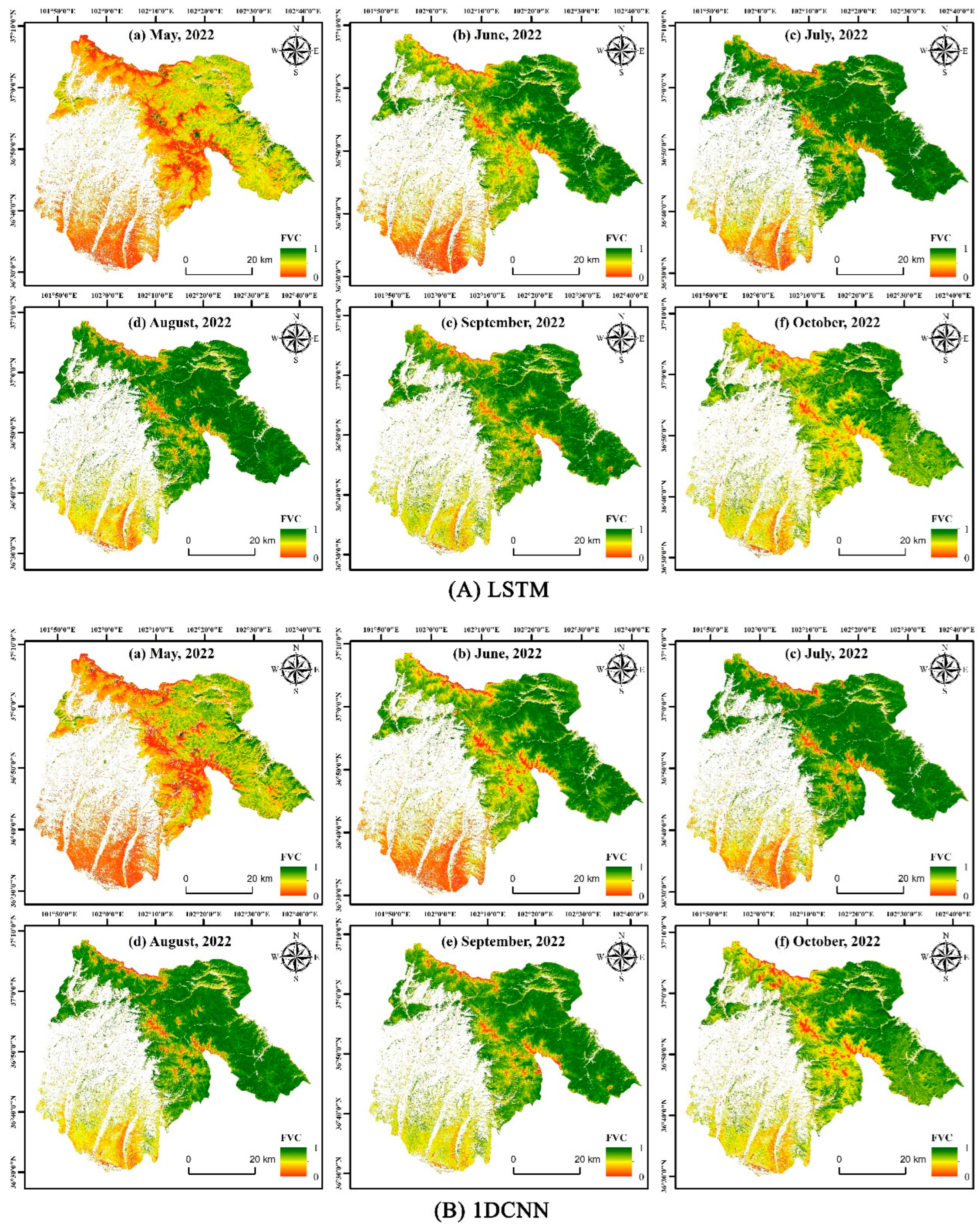
Figure 5A,B, respectively, show the spatio-temporal distribution of forest and grassland FVC in the mountain areas of Huzhu County for six periods in 2022, using the TL method based on LSTM and 1D-CNN networks. The FVC in the mountain areas of the study region presents distinct seasonal variations from May to October, with FVC gradually decreasing with increasing altitude. Comparing the vegetation cover extraction results of the LSTM and 1D-CNN models, the FVC estimates for June, July, and August are nearly similar. However, the FVC retrieval results of the two models show significant differences during periods of sparse vegetation in May and October.
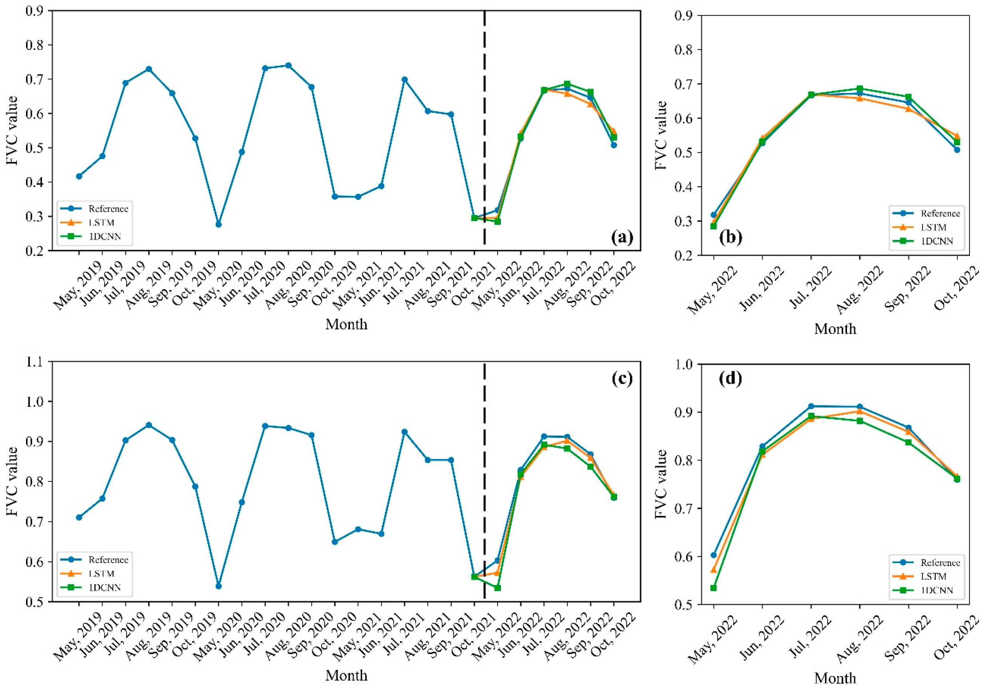
Figure 6 shows the temporal variation trend of the mean FVC time series inverted by the reference FVC, LSTM model, and 1D-CNN model. It can be observed that the FVC inversion results based on both models show a consistent trend with the actual reference FVC variation, with the LSTM method predicting FVC results that are closer to the reference FVC.
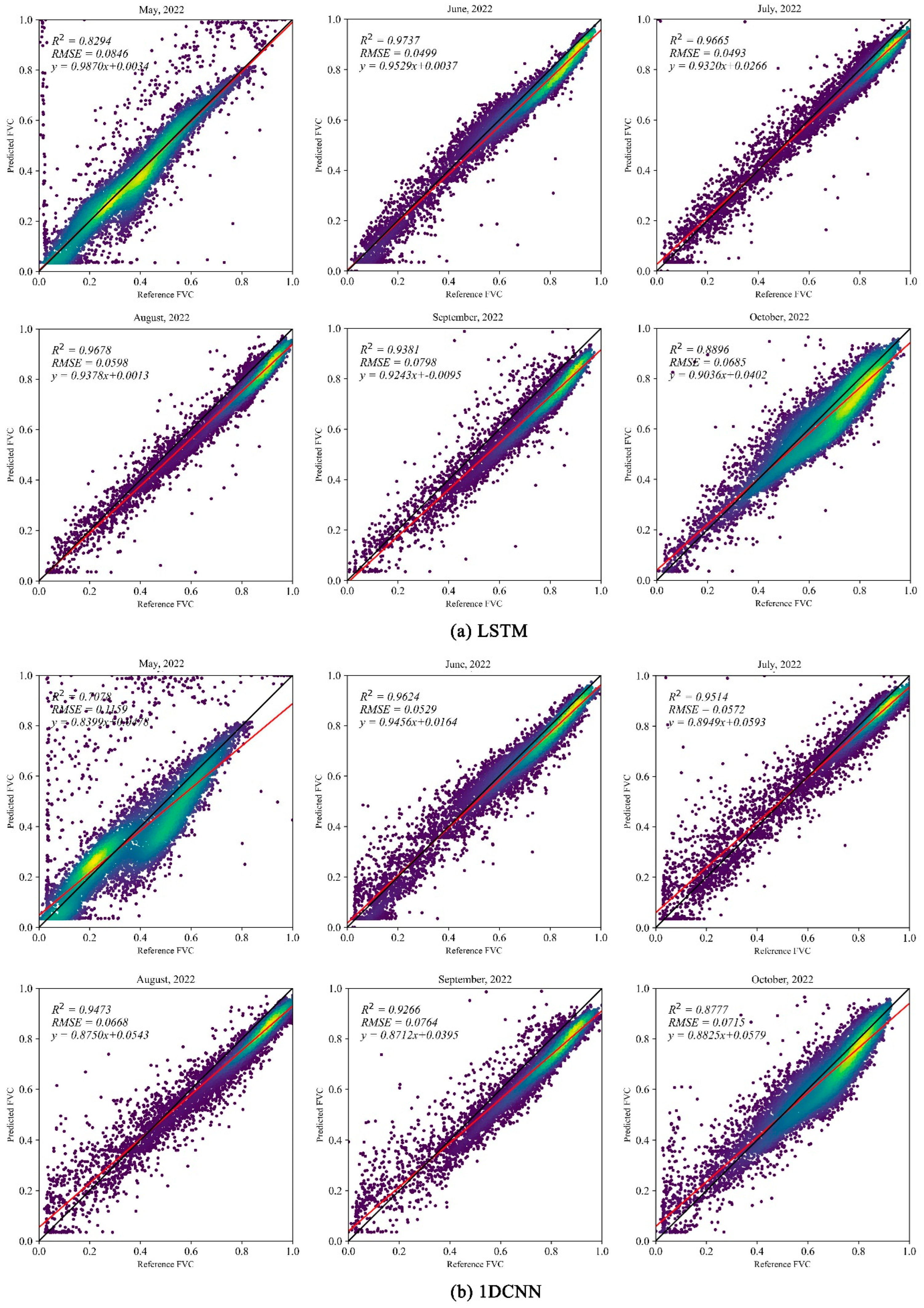
Table 3 presents the FVC prediction accuracy with LSTM and 1D-CNN models in grassland and forest areas, obtained by randomly selecting 9590 points in the mountain region of the study area for prediction. The mean R2 and RMSE values show that the performance of the LSTM model (grassland: R2 = 0.9108, RMSE = 0.0714; forest area: R2 = 0.8809, RMSE = 0.0581) is better than the 1DCNN model (grassland: R2 = 0.8722, RMSE = 0.0806; forest area: R2 = 0.847, RMSE = 0.065). Figure 7 are the scatter plots of the reference FVC vs. predicted FVC based on LSTM model (Figure 7a) and 1DCNN model (Figure 7b) from May to October 2022. The FVC retrieval accuracy of remote sensing image data of the model in June and July is higher, and the FVC retrieval accuracy difference between the two models is small. The FVC retrieval accuracy of the May image is the lowest, and the RMSE difference between the two models is approximately 0.03.

3.2. Importance Ranking of Features on FVC Retrieval

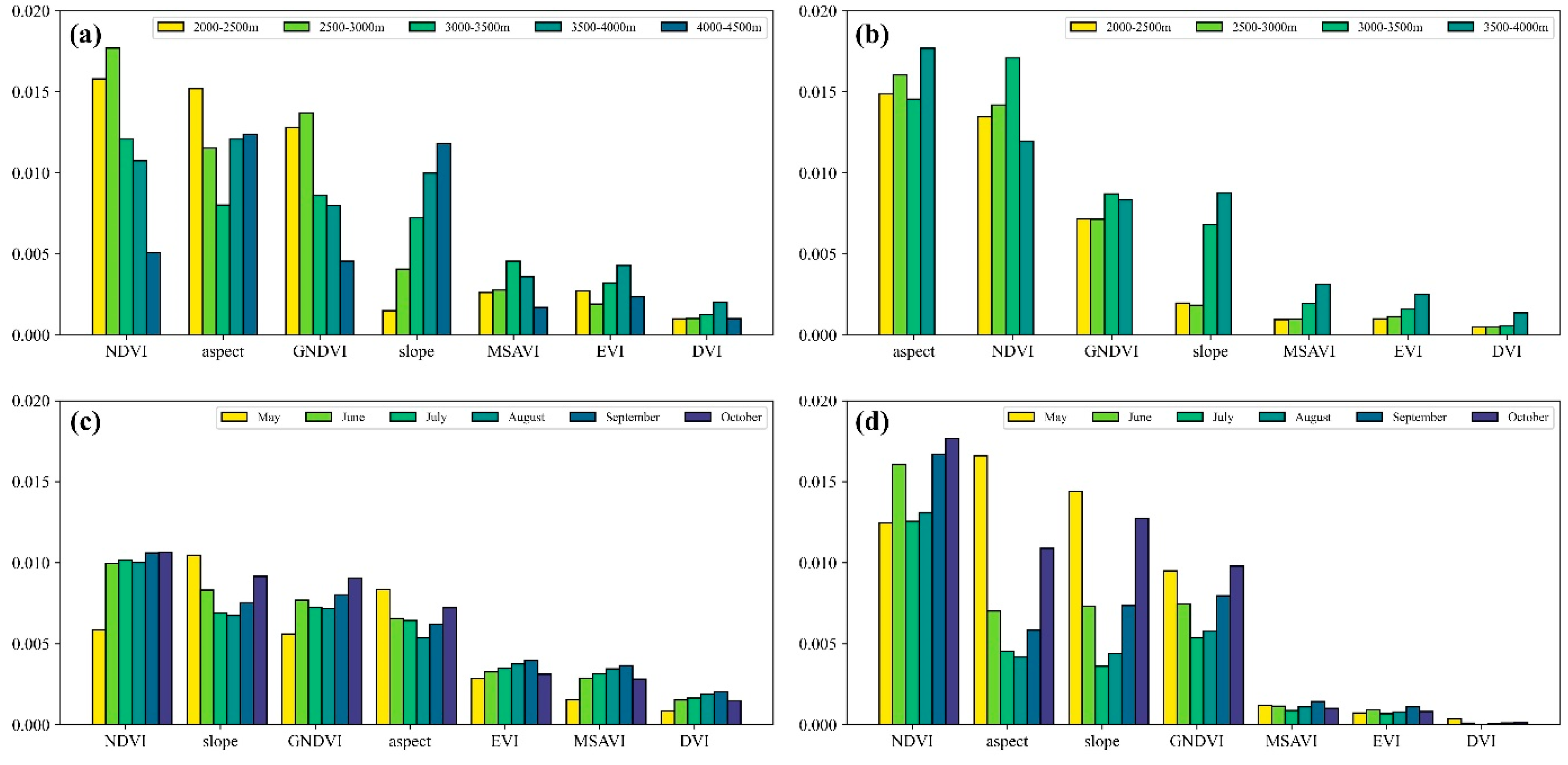
The importance ranking of features of different elevation gradients and months indicated that VIs and topographic factors had different impacts on FVC retrieval (Figure 8).
Under different altitude gradients, the four most important features in grassland are NDVI, aspect, GNDVI, and slope (Figure 8a), while in forest areas, the four most important features are aspect, NDVI, GNVDI, and slope (Figure 8b). MSAVI, EVI, and DVI are ranked as the least important features in both vegetation types. In grassland, NDVI and GNDVI exhibit a similar trend in importance, significantly influencing FVC prediction results. However, their importance gradually diminishes above 3000 m. The importance of slope increases with elevation, while the importance of aspect decreases first but then rises with increasing elevation.
Regarding the forest area, the importance of each feature showed a similar trend with the increase of the altitude gradient. Among the VIs, NDVI and GNDVI are the most important, and their importance is greatest at an altitude of 3000–3500 m. Concerning topographic factors, the aspect has the most significant impact on vegetation coverage. The slope is of little importance below an altitude of 3000 m, but it has a significant impact on FVC extraction in high-altitude areas above 3000 m.
Figure 8c,d shows the importance of topographic factors and VIs on the FVC retrieval results in each month of 2022, which reveals that the importance of feature variables also shows a seasonal pattern like the vegetation growth cycle. The change in the importance of VIs is basically similar to vegetation growth within a year, while the importance of topographic factors has an opposite trend, which is more pronounced in forest areas than grassland.

4. Discussion

4.1. Model Performance

The method, which uses PROSAIL and other RT models to establish the correspondence between Earth surface vegetation parameters and spectral features, makes up for the lack of high-precision samples in ML models, and it has begun to attract widespread attention in the quantitative retrieval of vegetation parameters [58]. In this paper, the FVC samples generated by the coupling model based on PROSAIL are validated with ground data, and their validation accuracy is compared with the accuracy of the high-resolution FVC samples generated by the dichotomy method.
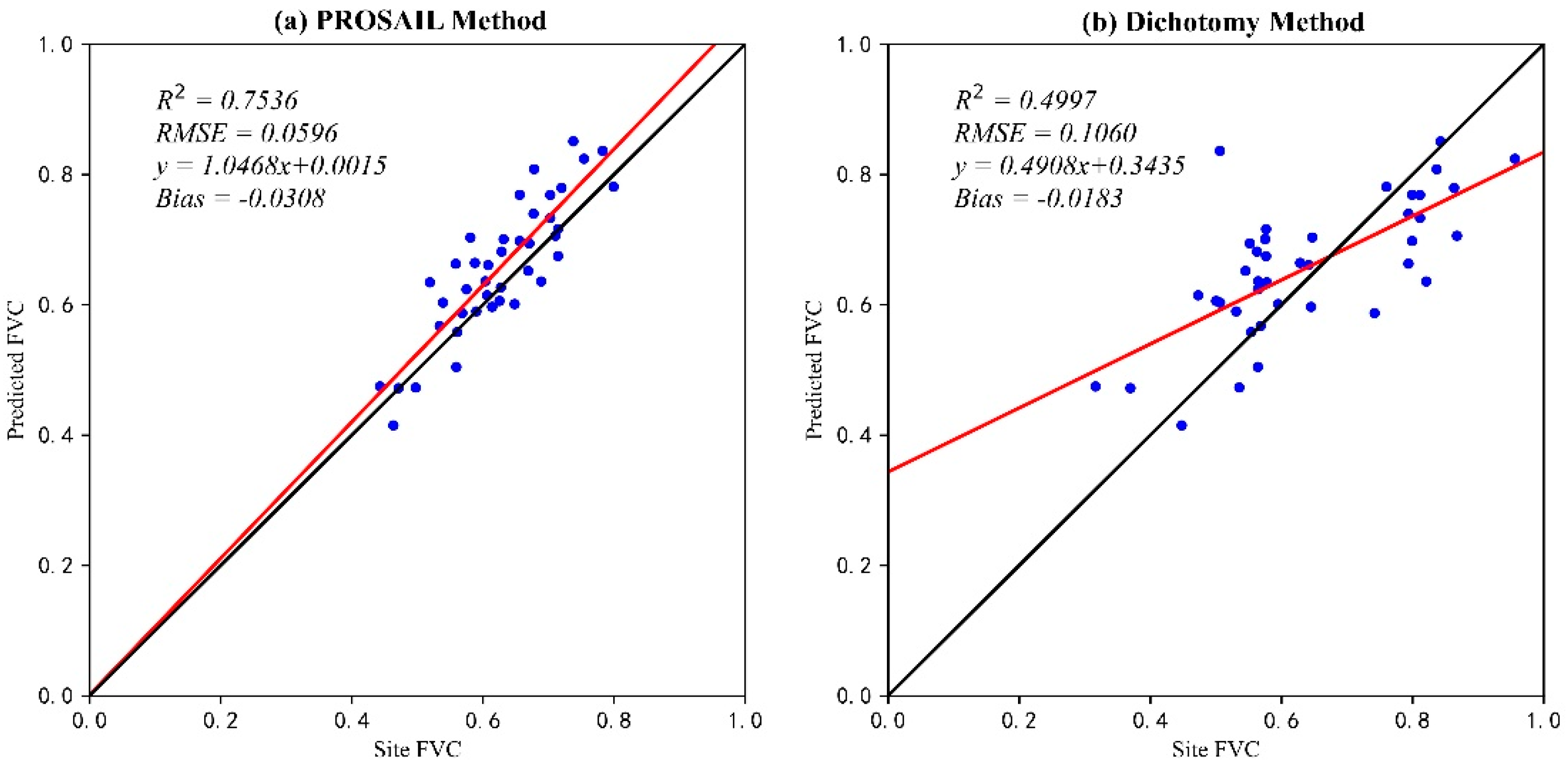
Figure 9 displays scatter plots comparing the accuracy of FVC samples generated through the proposed approach and the dichotomy model. In Figure 9a, the fitting line between the FVC samples generated by the proposed approach and the site FVC is closer to a 1:1 line (R2 = 0.7536, RMSE = 0.0596, Bias = −0.0308). It indicates that the accuracy of the proposed approach is better than that of the dichotomy method (R2 = 0.7536, RMSE = 0.0596, Bias = −0.0308), as shown in Figure 9b. These results demonstrate that the sample accuracy generated by the sample generator, which is based on PROSAIL simulation FVC, is guaranteed. It can provide high-precision training samples for the model in this paper.
By utilizing numerous simulated FVC samples and considering the mountain VIs and topographic factors such as slope and aspect, a pre-trained LSTM and 1DCNN network was used to create an FVC estimation model. This model was applied to multi-temporal HJ2-A/B remote sensing data. Upon analyzing the estimation results for forest and grass coverage, it was found that both LSTM and 1DCNN methods demonstrated high accuracy in FVC estimation for mountain areas. The model performed the best during the period from June to August when vegetation growth was at its highest. The complex structure of the LSTM network allowed it to extract interdependence between different time steps from time series data, giving it an advantage over the 1DCNN method in estimation accuracy. However, the 1DCNN method uses convolution and pooling operations that reduce computational training time compared to the LSTM method.
The model displayed the lowest RMSE in May; however, some sample points with low FVC are significantly overestimated. Based on the image, it can be observed that there is snow covering a significant portion of the area where the DEM exceeds 3500 m. This snow cover negatively impacts the distribution of sample points, which in turn affects the model’s ability to feature in the snow-covered region and causes a deviation in estimating the FVC. To enhance the model’s performance in future studies, it would be beneficial to incorporate additional variables such as temperature and precipitation.

4.2. Influence of Topographic Features on FVC Retrieval

The vegetation in high-altitude mountain regions is sensitive to various factors such as temperature, precipitation, soil, and illumination [59,60,61]. These factors are distributed differently across regions, which is indirectly affected by topographical features. The spatio-temporal statistical analysis of forest and grassland was carried out according to the classification standard of Table 4.
The result showed that the importance of topographical features varies with altitude and seasonality in mountain regions. Moreover, the contributions of these features to the estimation of FVC for forest and grassland are not the same.
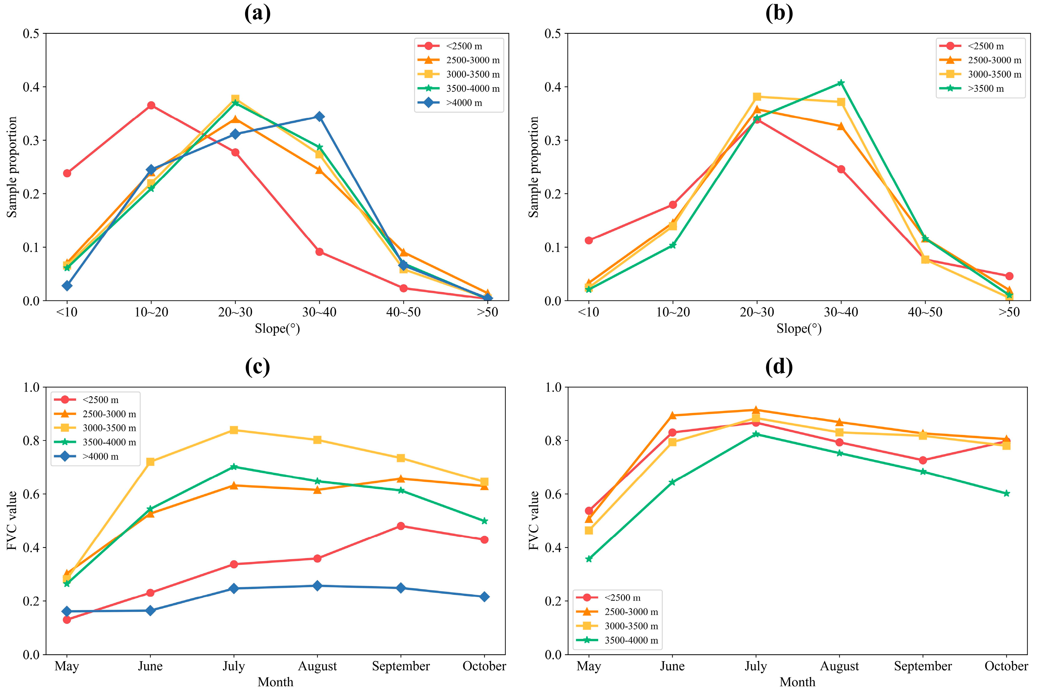
In general, slope significantly impacts the distribution of soil moisture and nutrients [62]. Figure 10a,b illustrate the distribution ratio of forest and grassland samples across various slope gradients. In regions below an altitude of 3000 m, the topography is generally characterized by gentle slopes with minimal undulations, resulting in effective water and nutrient retention in the soil. The slope gradient has a negligible effect on the FVC of forest and grassland in such areas. Shen [63] and De Castilho [64] also reported that topography has little influence on vegetation parameters, and biomass estimation results in regions with low topographic relief. Above 3000 m, the topographic undulation becomes more prominent with increasing altitude, resulting in reduced soil and water conservation capacity and a significant increase in the importance of slope gradient on the FVC of forests and grassland [61]. Furthermore, the impact of slope gradient on grassland is typically greater than that on forest land. This is attributed to the shallower root systems of grassland, which makes them less reliant on soil and, hence, more susceptible to slope gradients.
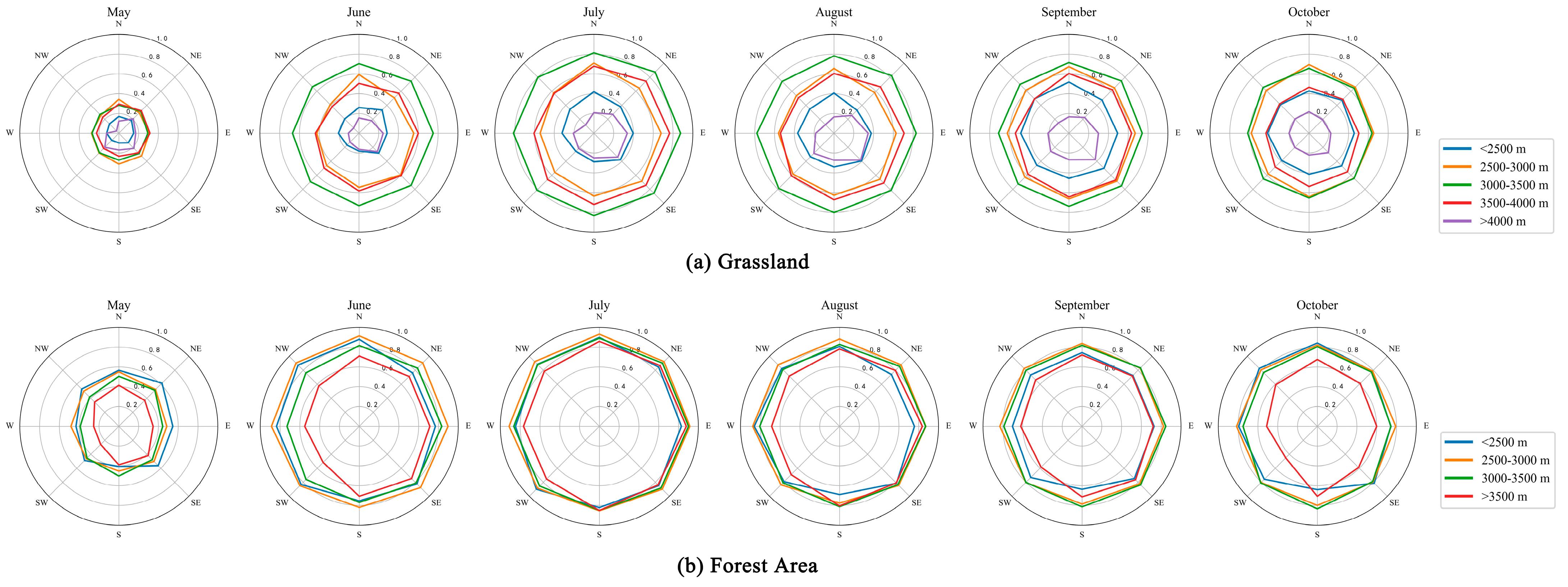
In various altitude gradients, aspect plays a significant role in determining forest and grass coverage. Aspect can influence the distribution and duration of solar radiation in mountain regions, leading to differences in FVC between sun and shadow slopes [62,65]. Figure 11 displays the average FVC distribution for eight orientations of forest and grassland between May and October 2022. At elevations below 3000 m, the vegetation cover on the shadow slopes (NE, NW) of the forested area is slightly higher than that on the sun slopes (SE, SW) (Figure 11b). Since the study area is located in the semi-arid area of the northern hemisphere, relatively high temperatures and dry microclimates tend to form on sun slopes [66,67], which promotes vegetation transpiration and soil water evaporation and inhibits the growth of vegetation on sunny slopes. However, the distribution of FVC on grassland slopes is contrary to that of forested slopes (Figure 11a). This is due to the dominance of forests as the vegetation cover type below 3000 m in the mountain area, which shades the low grassland and captures more sunlight than the grassland [68,69], thus inhibiting the vegetation cover of grassland. At elevations above 3000 m, the decline in temperature causes both forests and grasses to develop more on the sun slopes. With increasing elevation, alpine meadow gradually becomes the main vegetation cover type, which is less impacted by forest, and the tendency to grow on the sun slopes becomes more prominent.
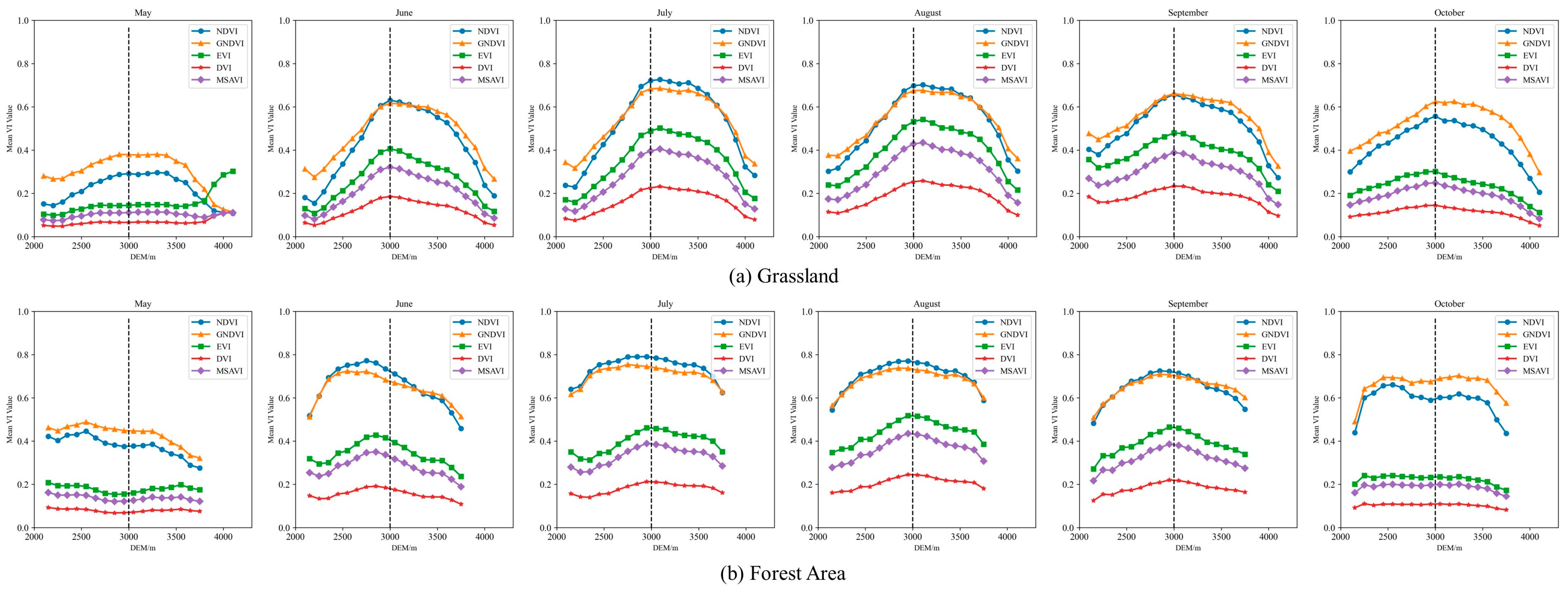
Moreover, vegetation growth can impact the importance of topographic features. Figure 10c,d and Figure 12 show highly similar trends in the variation of FVC and VI. The VI serves as a responsive indicator of climate change [5,70]. During the growing season (May to August), the temperature and precipitation in mountain regions are abundant, resulting in luxuriant vegetation. The VI has a direct influence on vegetation coverage, thus diminishing the importance of topographic factors. However, in September, the seasonal effect causes vegetation to become sparse, and it tends to thrive on sunlit slopes with adequate warmth and moisture [71], thereby gradually increasing the importance of topographic factors.

4.3. Influence of Pre-Training Sample Size

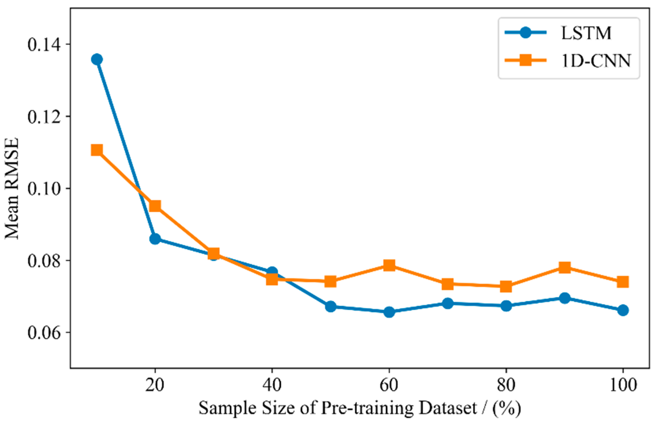
The pre-training of TL typically requires a significant amount of data, which directly affects the accuracy of quantitative retrieval of vegetation parameters. Although a large volume of training data can improve estimation accuracy, excessive data can result in issues such as information redundancy and prolonged training time, which can compromise both the accuracy and efficiency of the model [35]. In order to address these problems, using a random sampling method, Sentinel-2 time series datasets with varying data volumes (10%, 20%, 30%, …, and 100%) were utilized as input for pre-training the LSTM and 1D-CNN models. Subsequently, the model network weight parameters were fine-tuned using HJ-2A/B feature variables and corresponding FVC labels.
Figure 13 illustrates the trend of the RMSE of the FVC prediction results with varying pre-training sample sizes of the input model. Table 5 shows the FVC estimation accuracy of LSTM and 1DCNN models in all vegetation, grassland and forest areas under different pre-training sample sizes. The RMSE of FVC prediction for HJ-2A/B images in all phases was averaged for the study area. The FVC prediction accuracy improved as the pre-training sample size increased, with a sufficient sample size allowing for more comprehensive model training. Importantly, when the pre-training sample size exceeded 60% of the total sample size (approximately 90,000 sample points), the RMSE of FVC prediction no longer exhibited significant changes and gradually stabilized, indicating that the model had been fully trained.

4.4. Implications and Limitations

We propose an FVC estimation method based on a spatio-temporal transfer learning (TL) model, which utilizes simulated high-precision samples to pre-train the neural network and enables the estimation of FVC from high-resolution time series images in mountain regions. Both the LSTM and 1D-CNN models demonstrated high accuracy in extracting FVC of forest and grassland with varying topographic gradients in mountain regions, exhibiting strong cross-temporal sequence transferability. This transfer learning approach requires only a small number of samples for fine-tuning the pre-trained models, enabling the extraction of FVC from mountain remote sensing images in different temporal and spatial dimensions. The method can be further extended to extract high-precision vegetation parameters from larger regional scales.
The method proposed in this paper exhibits certain limitations. While it can provide the model with a large number of training samples, the generation of a considerable amount of simulated samples can result in data redundancy, which in turn may adversely impact the efficiency of model training and prediction [72]. Therefore, determining an appropriate sample size is a key research question that warrants further attention. Furthermore, due to geographic and seasonal constraints, this study examined only the peak period of vegetation growth (May to October). To extend the applicability of the model to other regions, a more comprehensive investigation of annual vegetation change patterns and consideration of various factors such as climate are imperative for fully unleashing the model’s potential.

5. Conclusions

In this study, we propose a novel method for estimating the FVC of forests and grassland in mountain areas based on spatio-temporal TL to address the issues of low sample accuracy and insufficient representation in the current FVC retrieval models. This method first combines the simulated FVC data generated by the PROSAIL model, the VI computed using the Sentinel-2 time series images, and the topographic data of the study area to establish a high-precision sample library in mountain areas. The samples are then divided by altitude and vegetation type and pre-trained using the LSTM and 1D-CNN models. Subsequently, the vegetation index and topographic data corresponding to the HJ2-A/B time series remote sensing images in 2022 are used to fine-tune the pre-training models, enabling the temporal and spatial transfer of images in mountain areas.
Based on the results, the simulated FVC samples demonstrate high accuracy. The LSTM and 1D-CNN models exhibit exceptional performance in estimating FVC from mountain image data with six temporal phases in 2022. However, due to their distinct structural characteristics, the LSTM model outperforms in classification accuracy but is more time-consuming during the retrieval process. The models achieve the highest prediction accuracy from June to August when mountain vegetation exhibits vigorous growth and minimal changes, enabling effective extraction of sample features. Conversely, from May to June, forest and grass coverage undergo rapid changes, particularly high-altitude snowline fluctuations, resulting in noticeable differences in the data between the two temporal phases. The deviation of the model extraction features leads to relatively large errors in FVC retrieval. Therefore, future studies could enhance the model by incorporating factors such as climate, snow cover, and precipitation to adapt to seasonal changes.
Topographic features are of great significance to the FVC retrieval in mountain areas. The analysis of the importance of feature variables demonstrates that slope and aspect are more crucial in areas with higher altitudes and relatively lower FVC. Furthermore, topographic factors have a greater impact on the FVC retrieval results during the period of vegetation dormancy or entering the dormancy period (May and October) in a year. Due to the differences between forest and grassland in mountain areas, the importance of topographic factors in the FVC retrieval of the two types of plants is different. The above conclusions explain why topographic factors need to be estimated in the retrieval of mountain FVC.
A subset of the pre-training samples can ensure the efficacy of the proposed method, indicating that the LSTM and 1D-CNN models can achieve stable performance using 90,000 pre-training samples in the study region. Notably, the LSTM-based model exhibits significantly superior predictive accuracy compared to the 1D-CNN-based model.
In summary, the proposed approach in this paper is advantageous in precisely estimating FVC in mountain areas that exhibit intricate climate patterns, substantial topographic fluctuations, and limited access to high-precision samples. This method enables the dynamic monitoring of mountain FVC in high-resolution remote sensing images and has the potential to expand its range, thereby furnishing more comprehensive data support for protecting vegetation in the fragile ecological regions of plateau mountains.

Author Contributions

Conceptualization, Y.H., T.L. and X.Z.; formal analysis, Y.H.; investigation, T.L. and X.Z.; methodology, Y.H.; project administration, H.Z.; software, Y.H.; supervision, X.Z.; validation, T.L. and X.Z.; visualization, R.L.; writing—original draft, Y.H.; writing—review and editing, Y.H., T.L., X.Z., Z.T., R.L., M.Z. and H.L. All authors have read and agreed to the published version of the manuscript.

Funding

This research was funded by the National Key R&D Program of China—Remote sensing assessment and capacity building of sustainable development in Hindu Kush Himalaya region (No. 2021YFE0117800).

Data Availability Statement

The satellite data used in this study are in the public domain and available from ESA (https://scihub.copernicus.eu/dhus/#/home, accessed on 1 October 2023), CRESDA (http://www.cresda.com/CN/, accessed on 1 October 2023), and STRM (https://srtm.csi.cgiar.org/srtmdata/, accessed on 1 October 2023).

Acknowledgments

We would like to thank Python for helping us design the neural networks, data analysis, and plotting. We also thank the journal’s editors and reviewers for providing insightful comments and suggestions for this paper.

Conflicts of Interest

The authors declare no conflict of interest.

References

  1. Grêt-Regamey, A.; Brunner, S.H.; Kienast, F. Mountain Ecosystem Services: Who Cares? Mt. Res. Dev. 2012, 32, S23–S34. [Google Scholar]
  2. Berger, F.; Rey, F. Mountain Protection Forests against Natural Hazards and Risks: New French Developments by Integrating Forests in Risk Zoning. Nat. Hazards 2004, 33, 395–404. [Google Scholar] [CrossRef]
  3. Messerli, B.; Ives, J.D. Mountains of the World: A Global Priority; Parthenon Publishing: Nashville, TN, USA, 1997. [Google Scholar]
  4. Carlson, T.N.; Ripley, D.A. On the Relation between NDVI, Fractional Vegetation Cover, and Leaf Area Index. Remote Sens. Environ. 1997, 62, 241–252. [Google Scholar]
  5. Gao, L.; Wang, X.; Johnson, B.A.; Tian, Q.; Wang, Y.; Verrelst, J.; Mu, X.; Gu, X. Remote Sensing Algorithms for Estimation of Fractional Vegetation Cover Using Pure Vegetation Index Values: A Review. ISPRS J. Photogramm. Remote Sens. 2020, 14, 364–377. [Google Scholar]
  6. Verger, A.; Baret, F.; Weiss, M. GEOV2/VGT: Near real time estimation of global biophysical variables from VEGETATION-P data. In Proceedings of the MultiTemp 2013: 7th International Workshop on the Analysis of Multi-temporal Remote Sensing Images, Banff, AB, Canada, 25–27 June 2013; pp. 1–4. [Google Scholar]
  7. Baret, F.; Weiss, M.; Verger, A.; Smets, B. ATBD for LAI, FAPAR and FCOVER from PROBA-V Products at 300 m Resolution (GEOV3). 2016. Available online: http://www.fp7-imagines.eu/media/Documents/ImagineS_RP2.1_ATBD-LAI300m_I1.73.pdf (accessed on 1 October 2023).
  8. Jia, K.; Liang, S.; Liu, S.; Li, Y.; Xiao, Z.; Yao, Y.; Jiang, B.; Zhao, X.; Wang, X.; Xu, S. Global Land Surface Fractional Vegetation Cover Estimation Using General Regression Neural Networks from MODIS Surface Reflectance. IEEE Trans. Geosci. Remote Sens. 2015, 53, 4787–4796. [Google Scholar]
  9. Wang, Y.; Tan, L.; Wang, G.; Sun, X.; Xu, Y. Study on the Impact of Spatial Resolution on Fractional Vegetation Cover Extraction with Single-Scene and Time-Series Remote Sensing Data. Remote Sens. 2022, 14, 4165. [Google Scholar] [CrossRef]
  10. Mu, X.; Zhao, T.; Ruan, G.; Song, J.; Wang, J.; Yan, G.; Mcvicar, T.R.; Yan, K.; Gao, Z.; Liu, Y.; et al. High Spatial Resolution and High Temporal Frequency (30-m/15-Day) Fractional Vegetation Cover Estimation over China Using Multiple Remote Sensing Datasets: Method Development and Validation. J. Meteorol. Res. 2021, 35, 128–147. [Google Scholar] [CrossRef]
  11. Mu, X.; Huang, S.; Ren, H.; Yan, G.; Song, W.; Ruan, G. Validating GEOV1 Fractional Vegetation Cover Derived From Coarse-Resolution Remote Sensing Images Over Croplands. IEEE J. Sel. Top. Appl. Earth Obs. Remote Sens. 2015, 8, 439–446. [Google Scholar] [CrossRef]
  12. Liu, D.; Jia, K.; Wei, X.; Xia, M.; Zhang, X.; Yao, Y.; Zhang, X.; Wang, B. Spatiotemporal Comparison and Validation of Three Global-Scale Fractional Vegetation Cover Products. Remote Sens. 2019, 11, 2524. [Google Scholar] [CrossRef]
  13. Florinsky, I.V.; Kuryakova, G.A. Influence of Topography on Some Vegetation Cover Properties. CATENA 1996, 27, 123–141. [Google Scholar] [CrossRef]
  14. Song, W.; Yan, K.; Mu, X.; Yan, G. Estimation and Uncertainty Analyses of Fractional Vegetation Cover (FVC) over Mountain Area. In Proceedings of the AGU Fall Meeting Abstracts, San Francisco, CA, USA, 12–16 December 2016; Volume 2016, p. B31E-0515. [Google Scholar]
  15. Adhikari, H.; Heiskanen, J.; Maeda, E.E.; Pellikka, P.K.E. The Effect of Topographic Normalization on Fractional Tree Cover Mapping in Tropical Mountains: An Assessment Based on Seasonal Landsat Time Series. Int. J. Appl. Earth Obs. Geoinf. 2016, 52, 20–31. [Google Scholar] [CrossRef]
  16. Gemmell, F. An Investigation of Terrain Effects on the Inversion of a Forest Reflectance Model. Remote Sens. Environ. 1998, 65, 155–169. [Google Scholar] [CrossRef]
  17. Soenen, S.A.; Peddle, D.R.; Coburn, C.A. SCS+C: A Modified Sun-Canopy-Sensor Topographic Correction in Forested Terrain. IEEE Trans. Geosci. Remote Sens. 2005, 43, 2148–2159. [Google Scholar] [CrossRef]
  18. Duguay, C.R.; LeDrew, E.F. Estimating Surface Reflectance and Albedo from Landsat-5 Thematic Mapper over Rugged Terrain. Photogramm. Eng. Remote Sens. 1992, 58, 551–558. [Google Scholar]
  19. Baret, F.; Clevers, J.G.P.W.; Steven, M.D. The Robustness of Canopy Gap Fraction Estimates from Red and Near-Infrared Reflectances: A Comparison of Approaches. Remote Sens. Environ. 1995, 54, 141–151. [Google Scholar] [CrossRef]
  20. Wittich, K.P.; Hansing, O. Area-Averaged Vegetative Cover Fraction Estimated from Satellite Data. Int. J. Biometeorol. 1995, 38, 209–215. [Google Scholar]
  21. Zhao, J.; Li, J.; Liu, Q.; Zhang, Z.; Dong, Y. Comparative Study of Fractional Vegetation Cover Estimation Methods Based on Fine Spatial Resolution Images for Three Vegetation Types. IEEE Geosci. Remote Sens. Lett. 2022, 19, 1–5. [Google Scholar]
  22. Montandon, L.; Small, E. The Impact of Soil Reflectance on the Quantification of the Green Vegetation Fraction from NDVI. Remote Sens. Environ. 2008, 112, 1835–1845. [Google Scholar] [CrossRef]
  23. Huang, R.; Chen, J.; Feng, Z.; Yang, Y.; You, H.; Han, X. Fitness for Purpose of Several Fractional Vegetation Cover Products on Monitoring Vegetation Cover Dynamic Change—A Case Study of an Alpine Grassland Ecosystem. Remote Sens. 2023, 15, 1312. [Google Scholar] [CrossRef]
  24. Maurya, A.K.; Nadeem, M.; Singh, D.; Singh, K.P.; Rajput, N.S. Critical Analysis of Machine Learning Approaches for Vegetation Fractional Cover Estimation Using Drone and Sentinel-2 Data. In Proceedings of the 2021 IEEE International Geoscience and Remote Sensing Symposium IGARSS, Brussels, Belgium, 11–16 July 2021; pp. 343–346. [Google Scholar]
  25. Song, D.-X.; Wang, Z.; He, T.; Wang, H.; Liang, S. Estimation and Validation of 30 m Fractional Vegetation Cover over China through Integrated Use of Landsat 8 and Gaofen 2 Data. Sci. Remote Sens. 2022, 6, 100058. [Google Scholar] [CrossRef]
  26. Chen, J.; Yi, S.; Qin, Y.; Wang, X. Improving Estimates of Fractional Vegetation Cover Based on UAV in Alpine Grassland on the Qinghai–Tibetan Plateau. Int. J. Remote Sens. 2016, 37, 1922–1936. [Google Scholar]
  27. Weiss, K.; Khoshgoftaar, T.M.; Wang, D. A Survey of Transfer Learning. J. Big Data 2016, 3, 9. [Google Scholar] [CrossRef]
  28. Pan, S.J.; Yang, Q. A Survey on Transfer Learning. IEEE Trans. Knowl. Data Eng. 2010, 22, 1345–1359. [Google Scholar] [CrossRef]
  29. Shin, H.-C.; Roth, H.R.; Gao, M.; Lu, L.; Xu, Z.; Nogues, I.; Yao, J.; Mollura, D.; Summers, R.M. Deep Convolutional Neural Networks for Computer-Aided Detection: CNN Architectures, Dataset Characteristics and Transfer Learning. IEEE Trans. Med. Imaging 2016, 35, 1285–1298. [Google Scholar]
  30. Wan, L.; Zhou, W.; He, Y.; Wanger, T.C.; Cen, H. Combining Transfer Learning and Hyperspectral Reflectance Analysis to Assess Leaf Nitrogen Concentration across Different Plant Species Datasets. Remote Sens. Environ. 2022, 269, 112826. [Google Scholar] [CrossRef]
  31. Khaki, S.; Pham, H.; Wang, L. Simultaneous Corn and Soybean Yield Prediction from Remote Sensing Data Using Deep Transfer Learning. Sci. Rep. 2021, 11, 11132. [Google Scholar]
  32. Yli-Heikkila, M.; Wittke, S.; Luotamo, M.; Puttonen, E.; Sulkava, M.; Pellikka, P.; Heiskanen, J.; Klami, A. Scalable Crop Yield Prediction with Sentinel-2 Time Series and Temporal Convolutional Network. Remote Sens. 2022, 14, 4193. [Google Scholar] [CrossRef]
  33. Wang, A.X.; Tran, C.; Desai, N.; Lobell, D.; Ermon, S. Deep Transfer Learning for Crop Yield Prediction with Remote Sensing Data. In Proceedings of the 1st ACM SIGCAS Conference on Computing and Sustainable Societies, San Jose, CA, USA, 20–22 June 2018; ACM: Menlo Park, CA, USA; San Jose, CA, USA, 2018; pp. 1–5. [Google Scholar]
  34. Astola, H.; Seitsonen, L.; Halme, E.; Molinier, M.; Lönnqvist, A. Deep Neural Networks with Transfer Learning for Forest Variable Estimation Using Sentinel-2 Imagery in Boreal Forest. Remote Sens. 2021, 13, 2392. [Google Scholar] [CrossRef]
  35. Yu, R.; Li, S.; Zhang, B.; Zhang, H. A Deep Transfer Learning Method for Estimating Fractional Vegetation Cover of Sentinel-2 Multispectral Images. IEEE Geosci. Remote Sens. Lett. 2022, 19, 1–5. [Google Scholar] [CrossRef]
  36. Holben, B.N. Characteristics of Maximum-Value Composite Images from Temporal AVHRR Data. Int. J. Remote Sens. 1986, 7, 1417–1434. [Google Scholar] [CrossRef]
  37. Marcial-Pablo, M.D.J.; Gonzalez-Sanchez, A.; Jimenez-Jimenez, S.I.; Ontiveros-Capurata, R.E.; Ojeda-Bustamante, W. Estimation of Vegetation Fraction Using RGB and Multispectral Images from UAV. Int. J. Remote Sens. 2019, 40, 420–438. [Google Scholar] [CrossRef]
  38. Zhang, X.; Liu, L.; Chen, X.; Gao, Y.; Xie, S.; Mi, J. GLC_FCS30: Global Land-Cover Product with Fine Classification System at 30 m Using Time-Series Landsat Imagery. Earth Syst. Sci. Data 2021, 13, 2753–2776. [Google Scholar] [CrossRef]
  39. Anderson, K.; Fawcett, D.; Cugulliere, A.; Benford, S.; Jones, D.; Leng, R. Vegetation Expansion in the Subnival Hindu Kush Himalaya. Glob. Chang. Biol. 2020, 26, 1608–1625. [Google Scholar] [CrossRef]
  40. Jacquemoud, S.; Verhoef, W.; Baret, F.; Bacour, C.; Zarco-Tejada, P.J.; Asner, G.P.; François, C.; Ustin, S.L. PROSPECT+SAIL Models: A Review of Use for Vegetation Characterization. Remote Sens. Environ. 2009, 113, S56–S66. [Google Scholar] [CrossRef]
  41. Rosema, A.; Verhoef, W.; Noorbergen, H.; Borgesius, J.J. A New Forest Light Interaction Model in Support of Forest Monitoring. Remote Sens. Environ. 1992, 42, 23–41. [Google Scholar]
  42. Gastellu-Etchegorry, J.-P.; Demarez, V.; Pinel, V.; Zagolski, F. Modeling Radiative Transfer in Heterogeneous 3-D Vegetation Canopies. Remote Sens. Environ. 1996, 58, 131–156. [Google Scholar] [CrossRef]
  43. Rouse, J.W.; Haas, R.H.; Schell, J.A.; Deering, D.W. Monitoring Vegetation Systems in the Great Plains with ERTS. NASA Spec. Publ. 1974, 351, 309. [Google Scholar]
  44. Gitelson, A.A.; Kaufman, Y.J.; Merzlyak, M.N. Use of a Green Channel in Remote Sensing of Global Vegetation from EOS-MODIS. Remote Sens. Environ. 1996, 58, 289–298. [Google Scholar]
  45. Huete, A.; Didan, K.; Miura, T.; Rodriguez, E.P.; Gao, X.; Ferreira, L.G. Overview of the Radiometric and Biophysical Performance of the MODIS Vegetation Indices. Remote Sens. Environ. 2002, 83, 195–213. [Google Scholar] [CrossRef]
  46. Richardson, A.J.; Wiegand, C.L. Distinguishing Vegetation from Soil Background Information. Photogramm. Eng. Remote Sens. 1977, 43, 1541–1552. [Google Scholar]
  47. Qi, J.; Chehbouni, A.; Huete, A.R.; Kerr, Y.H.; Sorooshian, S. A Modified Soil Adjusted Vegetation Index. Remote Sens. Environ. 1994, 48, 119–126. [Google Scholar] [CrossRef]
  48. Mazza, A.; Gargiulo, M.; Scarpa, G.; Gaetano, R. Estimating the NDVI from SAR by Convolutional Neural Networks. In Proceedings of the IGARSS 2018—2018 IEEE International Geoscience and Remote Sensing Symposium, Valencia, Spain, 22–27 July 2018; pp. 1954–1957. [Google Scholar]
  49. Kattenborn, T.; Leitloff, J.; Schiefer, F.; Hinz, S. Review on Convolutional Neural Networks (CNN) in Vegetation Remote Sensing. ISPRS J. Photogramm. Remote Sens. 2021, 173, 24–49. [Google Scholar] [CrossRef]
  50. Kiranyaz, S.; Ince, T.; Gabbouj, M. Real-Time Patient-Specific ECG Classification by 1-D Convolutional Neural Networks. IEEE Trans. Biomed. Eng. 2016, 63, 664–675. [Google Scholar] [CrossRef] [PubMed]
  51. Rußwurm, M.; Körner, M. Multi-Temporal Land Cover Classification with Long Short-Term Memory Neural Networks. The International Archives of the Photogrammetry. Remote Sens. Spat. Inf. Sci. 2017, 42, 551–558. [Google Scholar]
  52. Hochreiter, S.; Schmidhuber, J. Long Short-Term Memory. Neural Comput. 1997, 9, 1735–1780. [Google Scholar] [CrossRef]
  53. Gers, F.A.; Schraudolph, N.N.; Schmidhuber, J. Learning Precise Timing with LSTM Recurrent Networks. J. Mach. Learn. Res. 2003, 3, 115–143. [Google Scholar]
  54. Hüsken, M.; Stagge, P. Recurrent Neural Networks for Time Series Classification. Neurocomputing 2003, 50, 223–235. [Google Scholar] [CrossRef]
  55. Cao, J.; Zhang, Z.; Luo, Y.; Zhang, L.; Zhang, J.; Li, Z.; Tao, F. Wheat Yield Predictions at a County and Field Scale with Deep Learning, Machine Learning, and Google Earth Engine. Eur. J. Agron. 2021, 123, 126204. [Google Scholar] [CrossRef]
  56. Lundberg, S.M.; Lee, S.-I. A Unified Approach to Interpreting Model Predictions. In Proceedings of the 31st International Conference on Neural Information Processing Systems, Long Beach, CA, USA, 4–9 December 2017; Volume 30. [Google Scholar]
  57. Lundberg, S.M.; Erion, G.; Chen, H.; DeGrave, A.; Prutkin, J.M.; Nair, B.; Katz, R.; Himmelfarb, J.; Bansal, N.; Lee, S.-I. From Local Explanations to Global Understanding with Explainable AI for Trees. Nat. Mach. Intell. 2020, 2, 56–67. [Google Scholar] [CrossRef]
  58. Ali, A.M.; Darvishzadeh, R.; Skidmore, A.; Gara, T.W.; Heurich, M. Machine Learning Methods’ Performance in Radiative Transfer Model Inversion to Retrieve Plant Traits from Sentinel-2 Data of a Mixed Mountain Forest. Int. J. Digit. Earth 2021, 14, 106–120. [Google Scholar] [CrossRef]
  59. Allen, R.B.; Peet, R.K. Gradient Analysis of Forests of the Sangre de Cristo Range, Colorado. Can. J. Bot. 1990, 68, 193–201. [Google Scholar] [CrossRef]
  60. Busing, R.T.; White, P.S.; MacKenzie, M.D. Gradient Analysis of Old Spruce—Fir Forests of the Great Smoky Mountains circa 1935. Can. J. Bot. 1993, 71, 951–958. [Google Scholar] [CrossRef]
  61. Ojoyi, M.; Mutanga, O.; Odindi, J.; Abdel-Rahman, E.M. Application of Topo-Edaphic Factors and Remotely Sensed Vegetation Indices to Enhance Biomass Estimation in a Heterogeneous Landscape in the Eastern Arc Mountains of Tanzania. Geocarto Int. 2016, 31, 1–21. [Google Scholar] [CrossRef]
  62. Liu, B.; Biswas, S.R.; Yang, J.; Liu, Z.; He, H.S.; Liang, Y.; Lau, M.K.; Fang, Y.; Han, S. Strong Influences of Stand Age and Topography on Post-Fire Understory Recovery in a Chinese Boreal Forest. For. Ecol. Manag. 2020, 473, 118307. [Google Scholar] [CrossRef]
  63. Shen, B.; Ding, L.; Ma, L.; Li, Z.; Pulatov, A.; Kulenbekov, Z.; Chen, J.; Mambetova, S.; Hou, L.; Xu, D.; et al. Modeling the Leaf Area Index of Inner Mongolia Grassland Based on Machine Learning Regression Algorithms Incorporating Empirical Knowledge. Remote Sens. 2022, 14, 4196. [Google Scholar] [CrossRef]
  64. De Castilho, C.V.; Magnusson, W.E.; De Araújo, R.N.O.; Luizão, R.C.C.; Luizão, F.J.; Lima, A.P.; Higuchi, N. Variation in Aboveground Tree Live Biomass in a Central Amazonian Forest: Effects of Soil and Topography. For. Ecol. Manag. 2006, 234, 85–96. [Google Scholar] [CrossRef]
  65. Warren, R.J. Mechanisms Driving Understory Evergreen Herb Distributions across Slope Aspects: As Derived from Landscape Position. Plant Ecol. 2008, 198, 297–308. [Google Scholar] [CrossRef]
  66. Mokarram, M.; Sathyamoorthy, D. Modeling the Relationship between Elevation, Aspect and Spatial Distribution of Vegetation in the Darab Mountain, Iran Using Remote Sensing Data. Model. Earth Syst. Environ. 2015, 1, 30. [Google Scholar] [CrossRef]
  67. Jin, X.; Zhang, Y.; Schaepman, M.E.; Clevers, J.; Su, Z.; Cheng, J.; Jiang, J.; van Genderen, J. Impact of elevation and aspect on the spatial distribution of vegetation in the Qilian mountain area with remote sensing data. In Proceedings of the XXI Congress: Silk Road for Information from Imagery and Remote Sensing (ISPRS 2008), Beijing, China, 3–11 July 2008; The International Society for Photogrammetry: Hannover, Germany, 2008; pp. 1385–1390. [Google Scholar]
  68. Kumar, P.; Chen, H.Y.H.; Thomas, S.C.; Shahi, C. Linking Resource Availability and Heterogeneity to Understorey Species Diversity through Succession in Boreal Forest of Canada. J. Ecol. 2018, 106, 1266–1276. [Google Scholar] [CrossRef]
  69. Grime, J.P. Competitive Exclusion in Herbaceous Vegetation. Nature 1973, 242, 344–347. [Google Scholar]
  70. Purevdorj, T.S.; Tateishi, R.; Ishiyama, T.; Honda, Y. Relationships between Percent Vegetation Cover and Vegetation Indices. Int. J. Remote Sens. 1998, 19, 3519–3535. [Google Scholar] [CrossRef]
  71. An, S.; Zhang, X.; Chen, X.; Yan, D.; Henebry, G. An Exploration of Terrain Effects on Land Surface Phenology across the Qinghai–Tibet Plateau Using Landsat ETM+ and OLI Data. Remote Sens. 2018, 10, 1069. [Google Scholar] [CrossRef]
  72. Ma, X.; Lu, L.; Ding, J.; Zhang, F.; He, B. Estimating Fractional Vegetation Cover of Row Crops from High Spatial Resolution Image. Remote Sens. 2021, 13, 3874. [Google Scholar] [CrossRef]
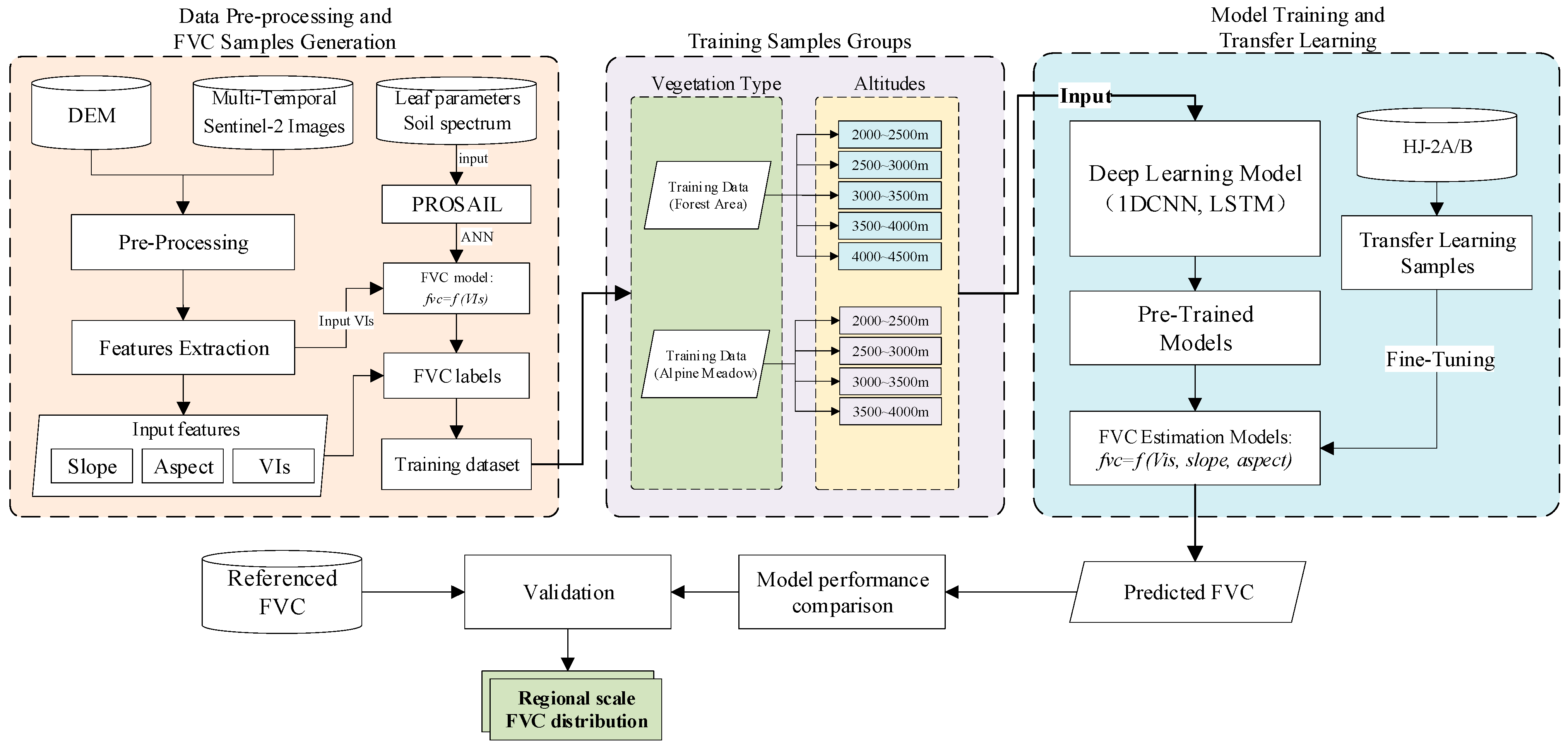
Figure 1. Flowchart of the mountain FVC retrieval based on TL methods.
Remotesensing 15 04857 g001
Figure 2. The remote sensing image (a), DEM map (b), and land cover map (c) of Huzhu County, Qinghai Province, China.
Remotesensing 15 04857 g002
Figure 3. The geographic location of Huzhu measurement area. (a) The green boxes are FVC measurement area. (b) The field photograph of the FVC measurement sample point. (c) The yellow dots are the site FVC points.
Remotesensing 15 04857 g003
Figure 4. The structure of 1DCNN (a) and LSTM (b).
Remotesensing 15 04857 g004
Figure 5. Spatial and temporal distribution pattern of estimated FVC in mountain area in Huzhu County from May to October 2022 based on LSTM (A) and 1DCNN (B) models.
Remotesensing 15 04857 g005
Figure 6. The FVC spatio-temporal variation charts of alpine meadow (a,b) and forest area (c,d) from May to October in 2019–2022. (b,d), respectively, show the predicted FVC of the LSTM model and 1DCNN model in the test set (a,b) and the change of the reference FVC.
Remotesensing 15 04857 g006
Figure 7. The scatter plots of the reference FVC vs. predicted FVC based on LSTM model (a) and 1DCNN model (b), respectively. A total of 9590 random points were generated in study area, and linear regression method was used to fit the reference FVC and predicted FVC.
Remotesensing 15 04857 g007
Figure 8. Importance ranking of the features in FVC retrieval for grassland and forest areas within different elevation areas (a,b) and bar plot of importance of features for grassland and forest areas from May to October in 2022 (c,d).
Remotesensing 15 04857 g008
Figure 9. The scatter plots of site FVC vs. predicted FVC (training samples) with PROSAIL method (a) and dichotomy method (b). The black diagonal is the 1:1 line, and the red line is the linear regression fitting line of the scatter point.
Remotesensing 15 04857 g009
Figure 10. (a,b) are the plot charts of sample number ratio of grassland and forest area sample points in different slope ranges in each altitude region. Figure (c,d) are plot charts of the monthly mean FVC changes of grassland and forest area in each altitude region.
Remotesensing 15 04857 g010
Figure 11. Polar coordinates of FVC distribution of grassland (a) and forest area (b) in different aspects from May to October 2022.
Remotesensing 15 04857 g011
Figure 12. Monthly trend chart of grassland (a) and forest (b) vegetation index with increasing altitude. In the figure, the horizontal axis represents the value of the vegetation index, and the vertical axis represents the DEM. The value of the vegetation index is the average of the vegetation index values of all sample points within each interval when the DEM is divided into 100 m intervals. The black dotted line X = 3000 is the dividing line of vegetation index change with altitude.
Remotesensing 15 04857 g012
Figure 13. Mean RMSE of LSTM and 1D-CNN method on HJ-2A/B data under different sample sizes of pre-training dataset.
Remotesensing 15 04857 g013
Table 1. Input parameters in the PROSAIL.
ModelParametersVariables NameRangeStep
PROSAIL C a b Chlorophyll a + b concentration (μg/cm2)20–8010
C m Dry matter content (g/cm2)0.005–0.0150.005
C a r Carotenoid content (g/cm2)0-
C w Equivalent water thickness (cm)0.005–0.0150.005
C b r o w n Brown pigment content0–1.50.5
SAIL N Leaf structure parameter1–20.5
L A I Leaf area index (m2/m2)0–70.5
A L A Average   leaf   inclination   angle   ( ° )30–7010
H o t Hot spot parameter0.1-
S Z A Solar   zenith   angle   ( ° )25–6510
Table 2. The number distribution of pre-training samples in grassland and forest areas.
Elevation(m)Sample Points
GrasslandForest Area
<250016842271
2500~300014,48438,203
3000~350025,63135,949
3500~400033,71715,731
>40002942
Table 3. The R2 and RMSE of FVC retrieval based on the LSTM model and 1DCNN model in grassland and forest, respectively.
MonthGrasslandForest Area
LSTM1DCNNLSTM1DCNN
R2RMSER2RMSER2RMSER2RMSE
May0.74980.10220.61490.13060.86750.06250.76200.0993
June0.96780.05440.95460.05790.9360.04480.90030.0475
July0.96320.05620.94400.06910.88570.04080.86620.0410
August0.97030.05960.94560.07170.92260.05990.89830.0613
September0.93710.08240.92150.07890.88440.07710.88300.0736
October0.87660.07330.85240.07530.78910.06320.77210.0673
Average0.91080.07140.87220.08060.88090.05810.84700.0650
Table 4. Classification of topographic variables in the study area.
SlopeAspect
ClassRange (°)DirectionRange (°)
1<10N337.5~22.5
210~20NE22.5~67.5
320~30E67.5~112.5
430~40SE112.5~157.5
540~50S157.5~202.5
6>50SW202.5~247.5
W247.5~292.5
NW292.5~337.5
Table 5. Retrieval accuracy of FVC of LSTM and 1DCNN models in all vegetation, grassland and forest areas under different pre-training sample sizes. The values in the table are the average of RMSE based on the FVC retrieval results of HJ-2A/B image data in 2022.
Sample SizeAll VegetationsGrasslandForest Area
LSTM1DCNNLSTM1DCNNLSTM1DCNN
10%0.13580.11050.16010.11650.10050.1004
20%0.08590.09500.08340.08690.08820.1009
30%0.08140.08180.07790.08130.08450.0810
40%0.07670.07470.08110.08430.07160.0634
50%0.06710.07410.07430.07280.05810.0739
60%0.06560.07850.07060.08140.05960.0782
70%0.06800.07340.07130.07810.06380.0639
80%0.06730.07270.07930.08120.05910.0633
90%0.06950.07800.07090.07710.06750.0780
100%0.06530.07350.07140.08060.05810.0650
Disclaimer/Publisher’s Note: The statements, opinions and data contained in all publications are solely those of the individual author(s) and contributor(s) and not of MDPI and/or the editor(s). MDPI and/or the editor(s) disclaim responsibility for any injury to people or property resulting from any ideas, methods, instructions or products referred to in the content.