Abstract
The exacerbation of wildfires, attributed to the effects of climate change, presents substantial risks to ecological systems, infrastructure, and human well-being. In the context of the Sustainable Development Goals (SDGs), particularly those related to climate action, prioritizing the assessment and management of the occurrence and intensity of extensive wildfires is of utmost importance. In recent times, there has been a significant increase in the frequency and severity of widespread wildfires worldwide, affecting several locations, including Australia, Italy, and the United States of America. The presence of complex phenomena marked by limited predictability leads to significant negative impacts on biodiversity and human lives. The utilization of satellite-derived data with neural networks, such as convolutional neural networks (CNNs), is a potentially advantageous approach for augmenting the monitoring capabilities of wildfires. This research examines the generalization capability of four neural network models, namely the fully connected (FC), one-dimensional (1D) CNN, two-dimensional (2D) CNN, and three-dimensional (3D) CNN model. Each model’s performance, as measured by accuracy, recall, and F1 scores, is assessed through K-fold cross-validation. Subsequently, T-statistics and p-values are computed based on these metrics to conduct a statistical comparison among the different models, allowing us to quantify the degree of similarity or dissimilarity between them. By using training data from Australia and Sicily, the performances of the trained model are evaluated on the test dataset from Oregon. The results are promising, with cross-validation on the training dataset producing mean precision, recall, and F1 scores ranging between approximately 0.97 and 0.98. Especially, the fully connected model has superior generalization capabilities, whilst the 3D CNN offers more refined and less distorted classifications. However, certain issues, such as false fire detection and confusion between smoke and shadows, persist. The aforementioned methodologies offer significant perspectives on the capabilities of neural network technologies in supporting the detection and management of wildfires. These approaches address the crucial matter of domain transferability and the associated dependability of predictions in new regions. This study makes a valuable contribution to the ongoing efforts in climate change by assisting in monitoring and managing wildfires.
1. Introduction
Recent technological advances in object recognition, deep learning, and remote sensing have revolutionized the way we can manage, detect, and track emergency and catastrophic events, such as wildfires, volcanic eruptions, and landslides [1,2,3]. In recent years, the increasing frequency and intensity of fires have made them a critical issue, significantly impacting the ecosystem and contributing to climate change [4,5]. Therefore, having a real or near-real-time forest fire detection system is vital to prevent significant losses and protect human lives. Satellite remote sensing is a cost-effective way to meet the need to detect, map, and study forest fires, and recent advances in sensors have made it easier [6,7]. For instance, the National Oceanic and Atmospheric Administration’s Advanced Very High-Resolution Radiometer and Landsat Thematic Mapper [8] were used to assess the burned areas, while NASA used MODIS and VIIRS data to provide a near-real-time global fire monitoring service [9]. In particular, hyperspectral (HS) data collected by satellite sensors provide high spatial and spectral resolution of the Earth’s surface, which can help identify wildfire [10], because it provides the necessary data in the infrared wavelengths to find burning areas and active fires [11]. Previous research examined EO-1 Hyperion data for temperature retrieval and fire detection over specific Alaskan boreal [12]. The analysis employed a Random Forest algorithm, achieving an F1 score of 0.97. Spectral analyses of a wildfire and biomass burning based on potassium emission signatures have been performed previously in published work using the laboratory, airborne, and space-borne HS-RS [13,14]; HS images have been used to characterise plumes, clouds, and fires [15].
This research employed PRISMA (PRecursore IperSpettrale della Missione Applicativa) [16] satellite data, a state-of-the-art hyperspectral imagery source, to reliably and comprehensively detect wildfires through convolutional neural networks. In addition, the IRIDE constellation project is slated to launch additional satellites with hyperspectral sensors in the upcoming five years (2027), making it Europe’s largest low-altitude multisensor Earth observation satellite space programme [17]. The project was founded by the Italian “Piano Nazionale di Ripresa e Resilienza” [18], through a partnership involving the Italian and European Space Agency and the Italian Ministry for Innovation and Digital Transition. On the one hand, HS imagery has the potential for the development of new analyses and methodologies; on the other hand, the exponential growth in the diversity and dimensionality of data presents new challenges for researchers. While these data represent a valuable resource, their organization and effective utilization pose significant difficulties. One of the primary challenges is data management and storage. Effectively handling, storing, and managing the extensive datasets generated by hyperspectral imagery require specialized infrastructure and significant computational resources.
In very recent years, a novel approach called HSI-VecNet was proposed in [19] for processing hyperspectral images (HSI) by learning vector representations from spectral-spatial data. It outperforms existing methods by addressing memory and distortion issues. The approach combines object classification and junction prediction to improve HSI vectorization. Again, in [20], a hyperspectral image segmentation method is introduced. It utilizes the Multi-Gradient based Cellular Automaton and an evolutionary algorithm (ECAS-II) to create customized segmenters from low-dimensional training data, outperforming existing methods in remote sensing hyperspectral imaging. In addition to these data management methods, Machine Learning (ML) techniques are an excellent solution for addressing this issue due to their remarkable performance in classification and segmentation tasks.
In this work, the potential offered by the combination of HS data (retrieved by PRISMA) and ML techniques has been investigated by analyzing different wildfire scenarios. When combined with neural network methodologies, PRISMA’s continuous spectral signature can lead to more accurate and broader classification feature extraction, avoiding confusion between different classes. For instance, in [21], R. U. Shaik et al. employed an automatic semi-supervised machine learning approach to distinguish between 18 different types of wildfire fuel using PRISMA hyperspectral imagery. Other works exploit PRISMA images to improve classification accuracy; in [22], the framework incorporates interpolation to compensate for the loss of noisy bands and utilizes Principal Component Analysis and Locality Preserving Projection for the extraction of hybrid features that preserve spatial information. Moreover, R. Grewal et al. [23] demonstrate that Deep Learning-based techniques, particularly spectral-spatial classification using CNN, outperform ML-based methods in HS classification, such as in [22], where a deep learning-based spectral-spatial framework for hyperspectral image classification is proposed. The framework integrates feature extraction, feature selection, and deep learning techniques to address the challenges of processing multidimensional data, resulting in improved performance compared to existing methods. At the end, in [24,25], a survey which encompasses hyperspectral image classification using machine learning techniques is provided.
Even though preliminary studies have already shown the successful usage of neural networks for hyperspectral imagery analysis [26,27,28], there are not many applications using neural network approaches for PRISMA hyperspectral data. Moreover, no previous studies (apart from the ones from the authors of this work) dealt with wildfire detection and analysis. Our earlier studies have demonstrated the potential for artificial intelligence, on-board computing, and satellite constellations to serve as interconnected components for future services that should aid in monitoring and prompt responses to wildfire events. The quality of the information that can be extracted from PRISMA HS imagery was investigated in [29], where analytical methodologies were proposed to locate wildfires and estimate the temperature of active fire pixels. At the same time, we showed the possibility of implementing Trusted Autonomous Satellite Operations [30,31,32] by utilizing artificial intelligence [33,34] on-board satellites with astrionics for data processing [35,36,37]. For the purpose of providing real-time or near real-time disaster management, the same has been used in Distributed Satellite Systems [38,39,40].
This investigation aims to contribute to the advancement of research by contributing in the following ways, starting from the promising results that were achieved by combining ML and HS data:
- Presenting the potential of deep learning techniques to detect spectral dependencies in wildfire situations. Different approaches are proposed based on spectral and spatial analyses.
- Using models trained in Australia and Sicily, performing generalization tests in Oregon to assess the methodology’s generalization capacity. The information contained in the trained networks is transferred to another domain, performing inferences in a different ecosystem, with respect to the one used for the training.
- Discussing the potential to make efficient use of ML-based methodologies in order to deliver notifications in the event that a new wildfire breaks out. With this regard, the computational performances of the proposed methodologies are discussed.
This paper is organized as follows. In Section 2, the dataset is described in terms of areas of interest and hyperspectral PRISMA imagery. The description of the methodology is provided in Section 3, where the four neural networks are introduced. The results of the training (using datasets from Australia and Sicily) and the testing (in Oregon) are reported in Section 4, while Section 5 deals with the discussion of the numerical findings. Finally, concluding remarks are provided in Section 6.
2. Dataset Definition
This section provides an overview of the PRISMA hyperspectral data and the regions of interest that were utilized in training, validating, and testing the neural network models.
2.1. PRISMA Data
PRISMA was launched on 22 March 2019, with a hyperspectral and panchromatic payload that can produce extremely high-quality HS images. The camera has 173 channels of Short-Wave InfraRed (SWIR) and 66 channels of Visible and Near InfraRed (VNIR) in the spectral range of 0.4–2.5 nm. With an accuracy of ±0.1 nm, the average spectral resolution across the entire range is less than 10 nm. The panchromatic camera’s ground sampling distance for PRISMA images is 5 m, while the hyperspectral camera is 30 m. The PRISMA data are made available for free for research purposes by the Italian Space Agency [41]. HS and panchromatic data are delivered in the HDF5 format in four levels:
- L1, radiance at the top of the atmosphere, radiometrically and geometrically calibrated;
- L2B, radiance geolocated at-ground;
- L2C, reflectance geolocated at-surface product;
- L2D, geocoded version of the Level 2C product.
In this investigation, we made use of PRISMA Level 2D data. For detailed information on PRISMA product specifications, please refer to the PRISMA product specifications document at https://prisma.asi.it (accessed on 15 July 2023).
2.2. Areas of Interest
The current investigation is concentrating its efforts on collecting data from three different continents, Oceania (New South Wales, Australia), North America (Oregon, United States of America), and Europe (Sicily, Italy), as shown in Figure 1. HS imagery was acquired in Australia, Sicily, and Oregon on 27 December 2019, 5 August 2021, and 17 July 2021, respectively.
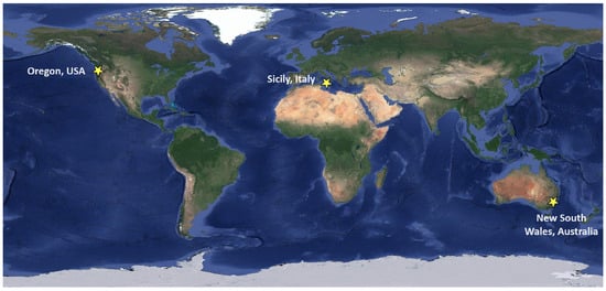
Figure 1.
Selected areas of interest for investigation.
These locations have witnessed significant impacts on human lives, property, and the environment, emphasizing the need for improved fire management practices. Their diverse geographic, environmental, and ecological factors contribute to unique and complex wildfire concerns and are used to verify the effectiveness of the proposed approach in diverse ecosystems. Therefore, these geographic areas emerge as very promising testbeds for conducting a rigorous evaluation of the effectiveness of our proposed methodology within a different spectrum of ecosystems. In particular, by examining the Global Agro-Ecological Zones (GAEZ) map made available by the Food and Agriculture Organization of the United Nations (FAO) (at https://gaez.fao.org/, accessed on 5 June 2023), it can be noticed that these regions comprise distinct agro-ecological zones. Specifically, the map emphasizes that Oregon is situated in a relatively more humid region compared to the others, while the Australian region stands out as the driest among them. This further underscores the pronounced ecological diversity and intricacy inherent in these territories.
The reference pixels employed for training, validation, and testing of the CNN were identified meticulously and manually through an analysis of the spectral characteristics exhibited by pixels within the images of each area of interest. Within these three images, seven distinct categories are discerned: fire, smoke, burned areas, vegetation, bare soil, water, and clouds (see Table 1). However, it is worth noting that the first five categories were mostly identified in both the Australian and Oregon images, whereas in the case of the Sicily image, the presence of clouds and water is evident in this area. Once the dataset was created, pixels from Australia were combined with the cloud and water classes from Sicily to assess the training and validation datasets. Oregon and three hot spots corresponding to small pastoral fires in Sicily were used as the test dataset. Due to the manual nature of the dataset labeling process, it was not feasible to comprehensively label the entirety of the images.

Table 1.
Number of labelled reference pixels in Australia, Sicily, and Oregon.
2.2.1. New South Wales, Australia
Australia is one of the world’s most fire-prone countries. The climate of the nation is hot and dry, and the vegetation becomes especially flammable. Australia has a long history of devastating wildfires, colloquially known as bushfires. Wildfires thrive in the country’s broad landscapes, extensive forested sections, and dry climate. Australia’s distinctive flora and fauna, notably eucalyptus trees rich in highly flammable oils, are contributing to the intensity and swift spread of fires. The horrific 2009 “Black Saturday” bushfires and the 2019–2020 blaze season are great examples of how wildfires may have disastrous effects on populations, wildlife, and ecosystems. The first area of interest in this study is Ben Halls Gap National Park in Australia, located about 250 km north of Sydney in the New South Wales region. This park is known for its cool temperatures, high elevation and significant rainfall. However, in 2019, the area was hit by a severe wildfire due to a combination of warm temperatures, high winds, and low humidity. An RGB composite of the region was included in this study, with labelled points used to test and train our CNN (as shown in Figure 2). Within the composite, we located two major fires: one in the southern portion near 151.2°E, 31.59°S, and the next in the northern portion near 151.3°E, 31.46°S. Additionally, 151.18°E, 31.39°S in the north-west is the location of a smaller active fire. On 27 December 2019, PRISMA acquired the image over this area of interest. The first row of Table 1 shows how many labelled pixels were found in the Australia image, where the Water and Clouds classes were not labelled as they are absent.
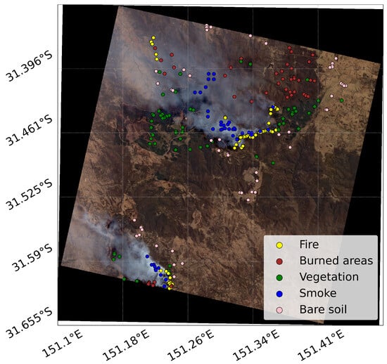
Figure 2.
RGB PRISMA composite image in the Australian area of interest with input labelled points.
2.2.2. Oregon, USA
The United States of America (USA) is highly susceptible to wildfires due to its abundant wilderness and typically humid and hot weather conditions. The country has a history of experiencing numerous extreme wildfire events, with distinct wildfire patterns across different regions. Western states, including California, Oregon, and Colorado, frequently face severe wildfires attributed to a combination of factors such as arid climates, elevated temperatures, and extensive wildland–urban interfaces. The US region investigated in this research is located in the Fremont-Winema National Forest in Oregon (42.616°N, 121.421°W). The Bootleg fire, which was started by lightning on 6 July 2021, garnered widespread media attention for two main reasons. First, a high-voltage transmission line that links hydroelectric power plants in the Pacific North-West to electricity demand centres in Los Angeles, California, was nearby when the fire started. Second, a concentration of dry forest (more information can be found at https://inciweb.nwcg.gov/incident/7609/, accessed on 3 May 2022) was created as a result of the fire spreading quickly due to a combination of grass, shrubs, and timber that a beetle kill had previously impacted. On 15 July, aerial data collection was impeded by pyrocumulus clouds that formed along the southeastern edge of the Bootleg fire. The Bootleg fire covered a region of about 1008 km as of 17 July 2021, according to satellite images, and it continued to burn unchecked until October 1, 2021, when it covered a distance of 1674 km. The RGB composite of the search area and labelled points using the transfer learning approach test is shown in Figure 3 along with the number of labelled pixels found in the Oregon image, which is displayed in the second row of Table 1. Similarly to the Australian case, the water and cloud classes are absent in Oregon as well. Additionally, the smoke pure pixel class is smaller in size compared to the other classes, containing only nine instances.
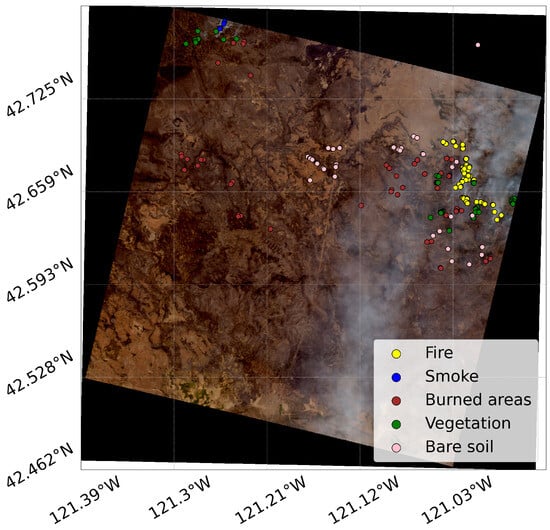
Figure 3.
RGB PRISMA composite image with input labelled points in the Oregon area of interest.
2.2.3. Sicily, Italy
Italy is highly susceptible to wildfires due to a combination of vegetation cover and climate regimes, particularly during summer. Human-caused wildfires are also common occurrences in the country. Italy’s hot and dry summers, particularly in its coastal regions, contribute to the prevalence of wildfires. The country’s landscapes, notably in coastal and mountainous areas, are prone to ignition and rapid fire spread. As a result, wildfires pose significant challenges to local governments in managing urban–wildland interactions and preserving historical sites and diverse ecosystems. Notable examples of major fire occurrences in Italy include the 2017 Central Italy wildfires and the 2007 Southern Italy wildfires. These incidents emphasize the need for effective wildfire management strategies to safeguard communities, cultural heritage, and natural resources from the devastating impacts of wildfires. Summer 2021 was very dry in Italy, with temperatures far above the seasonal average and creating favourable conditions for wildfires with the highest number of fires in Europe [42], with 14 of the 49 largest fires registered across Europe, the Middle East, and North Africa. The third study area of this paper is situated in the South-Central region of Sicily, with coordinates approximately at 37.429°N and 14.249°E. PRISMA acquisition was planned under very urgent acquisition (within the project “Progetto per Sviluppo di prodotti iperspettrali prototipali evoluti” Rif: CMM-PRO-18-013, funded by Italian Space Agency) aiming to map the fire front on the region, but the large fire was suppressed at the time of PRISMA acquisition (Figure 4).
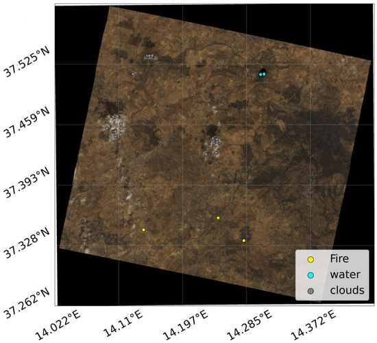
Figure 4.
RGB PRISMA composite image in the Sicily area of interest with input labelled points.
However, three hot spots were detected by using the Hyperspectral Fire Detection Index (HFDI) [29,43,44], and verified during the manual inspection of the pixels spectrum, by using both the NIR-SWIR color composition and spectral behaviour of active fires’ reflectance. The presence of clouds and water are evident in this area, which has been utilized for training the CNN in detecting and distinguishing between these two categories; meanwhile, the three hot spots corresponding to small pastoral fires were excluded from the dataset; they were utilized to validate the generalization ability assessment process, i.e., to verify if the CNN trained on Australia fires can also successfully detect the small fires in Sicily. Figure 4 reports the RGB composite of the research area along with the water and cloud points that were used for the training and the three small fires in the south of the area. The last row of Table 1 reports the total number of labelled pixels found in the Sicily image. The Sicily dataset primarily serves as the main source for training and evaluating the water and cloud classes, whereas only a limited number of three fire pixels are detected.
3. Methods
Due to the limited number of labeled pixels, we aim to assess the performance of the neural network through a comparative analysis of different approaches to determine the best one. We use cross-validation and statistical comparison to evaluate the performance of each method. In this context, the fully connected approach serves as the reference due to its simplicity, while the other approaches, including 1D CNN, 2D CNN, and 3D CNN, progressively increase in complexity. This section presents these various neural networks (Figure 5) and their evaluation methods.
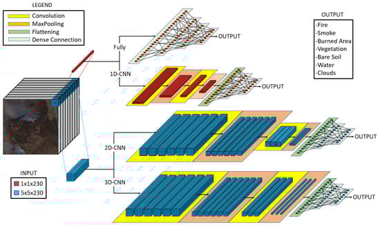
Figure 5.
Architectures of the proposed neural networks.
3.1. Architecture of the Models
The fine-tuning of hyperparameters involved iterative adjustments, including trial and error techniques. This systematic refinement aimed to strike a balance between complexity and efficiency while continuously monitoring validation dataset results. Importantly, the four networks utilized a similar structural design, featuring three hidden layers and a softmax output layer. This uniformity allowed for a direct and meaningful comparison among the networks. All of the models were trained using the Adam optimizer and the categorical cross-entropy loss function. The networks have been implemented using Python and Keras. The segmentation analysis is performed by running the models for each pixel in the image. All experiments were conducted on a personal computer equipped with 12 GB of RAM, an Intel Core i7-12700H 2.70 GHz CPU from the 12th Generation, and an NVIDIA GeForce RTX 3080 Ti GPU with 16 GB of dedicated RAM (manufactured by Intel and NVIDIA Corporation, Santa Clara, California, United States). All of the models were trained with a maximum of 200 epochs and an automatic early stopping criterion based on a patience parameter of 30 epochs.
3.1.1. Fully Connected Model
The architecture of the FC neural network consists of three identical hidden layers, except for the parameter defining the number of units, which is progressively reduced. The model processes input data with 230 features and has seven output classes. It consists of three dense layers with decreasing units (900, 450, and 225) and ReLU activation. The model’s weights are initialized using the “Henormal” initializer, and “L2” regularization is applied to prevent overfitting. The output layer (D4) has 7 units with a softmax activation for class probabilities. The model is compiled using the Adam optimizer with a learning rate of and categorical cross-entropy loss.
3.1.2. One-Dimensional Convolutional Neural Network
The 1D-CNN architecture was described and exploited in previous works [30,35,36,39,45,46,47]. Its input consists of pixel spectral signatures, represented as an array with a length of 230, defined by SWIR and VNIR PRISMA channels. The first hidden layer consists of a one-dimensional convolutional layer with 128 filters, a kernel equal to 3, the same padding, an L2 kernel regularizer with , and a ReLU activation function. This layer is followed by a max pooling layer with a pool size of 2 and a stride of 2. The sequence comprising convolutional and max pooling layers is replicated immediately thereafter, but with 64 filters in the convolutional layer. Then, the output of the flattening layer is passed through a fully connected layer of 32 units equipped with a ReLU activation function. Lastly, the model includes a dense unit with a softmax activation function for multi-class classification purposes.
3.1.3. Two-Dimensional Convolutional Neural Network
The model takes images with 230 channels as input and consists of two convolutional layers with kernels, and 128 and 64 filters, respectively, followed by max pooling layers. It includes a dropout layer with a 50% dropout rate to prevent overfitting. A flatten layer is used to reshape the output from the last max pooling layer into a 1D vector. Subsequently, there are two dense (fully connected) layers. The first dense layer has 32 units with a ReLU activation function, and the second dense layer has 7 units with a softmax activation function to produce class probabilities. The model is trained using the Adam optimizer with a learning rate of and L2 regularization with a lambda value of .
3.1.4. Three-Dimensional Convolutional Neural Network
The 3D-CNN input is represented by a hyperspectral cube wherein the central pixel is labelled, and neighbouring pixels are included, referenced from their spectral signatures. As presented in Figure 5, the first hidden layer is a 3D convolutional layer with 128 filters, kernel equal to , same padding, L2 kernel regularizer with , and ReLU activation function. This layer is followed by a max pooling layer with a pool size of 3 and a stride of 1. Afterwards, the data flows through another 3D convolutional layer with 64 filters, kernel equal to , the same padding, an L2 kernel regularizer, and a ReLU activation function. Similarly to the 1D-CNN architecture, this layer is followed by another max pooling layer with the same parameters. The output is then processed through a flattening layer before arriving at a fully connected layer of 32 units equipped with a ReLU activation function. Lastly, the model includes a dense unit with a softmax activation function for multi-class classification purposes.
3.2. Cross-Validation and Statistical Comparison
Cross-validation is a fundamental technique used in neural networks and other areas of machine learning to evaluate model performance and mitigate the risk of overfitting [48]. It consists of dividing the available dataset into multiple subsets, called folds, and using these folds iteratively to train and evaluate the model. The main reason for using cross-validation is to evaluate the ability of a neural network to generalize to unseen data. By training and evaluating the model on different subsets of data, cross-validation provides a more reliable estimate of model performance than a single train-test split. To split the dataset for each network, the “KFold” function from the “Scikit-learn” [49] library was exploited to split the dataset (Table 1) into five folds for each network. This specific approach was repeated five times, resulting in a total of twenty-five training iterations for each individual network.
Once cross-validation was performed for each model, the p-value and the t-statistic were calculated pairwise to compare the networks. Specifically, the p-value, a crucial statistical measure, quantified the evidence against the null hypothesis, positing no significant difference in network performance. By computing the p-value for each network pair, the investigation determined whether a statistically significant discrepancy existed in their performance. The t-statistic is essential for comparing the performance of two networks and determining which one is better based on the direction of the difference between their averages. It is a statistical measure used to test hypotheses about population means, especially in cases with small sample sizes or unknown population standard deviations.
3.3. Models’ Performances on the Test Dataset
The evaluation of a machine learning model’s generalization ability and its application in regions beyond the training domain are critical aspects of geographical classification problems. Generalization refers to the model’s capacity to perform well on unseen data from the same distribution as the training data. When a model is trained in one geographical region and subsequently tested in distant regions, it provides a valuable test of its generalization capability. By assessing the model’s performance in geographically distinct regions, one can gauge its adaptability to variations in geographical features and ascertain whether it can provide meaningful predictions in new settings.
Moreover, the scenario of testing the model in geographically distant regions with different characteristics can also be viewed as an example of transfer learning. Transfer learning involves leveraging knowledge obtained from one task or domain to enhance performance on a related task or domain. This challenge aligns with the essence of transfer learning, as the model must adjust to varying geographical features, climatic conditions, and other factors in the testing regions, to yield reliable results.
The combined assessment of generalization ability and transfer learning implications in geographical classification problems is crucial for gauging the model’s robustness and potential real-world applicability in regions with diverse geographical traits. Two generalization and transfer learning test cases were considered in this work. In Sicily, cloud and water pixels were selected to take part in the training dataset so that, here, both the generalization and the transfer learning approaches are reduced slightly, as some pixels (even though only for a few classes) were used in the training process. For the Sicily case, only a visual inspection of the results is reported without providing a numerical evaluation of the model performances. However, the model was transfer-learned in Oregon without additional re-training or fine-tuning. The accuracy of this transfer learning approach is evaluated using labelled pixels from the Oregon area, which served as an unseen scenario.
4. Results
In this section, the results of the different models in terms of their performance and similarity are reported. Cross-validation is used to assess the performance of the models, while statistical comparisons (p-value and t-statistic methods) are employed to gauge the degree of similarity among the various neural networks. Furthermore, performance metrics related to inference time and the number of parameters are also considered as additional factors for comparing the various models. At the conclusion, predictions for each image are provided to ease visual inspection and support final considerations based on the visual assessment.
4.1. Cross-Validation
Cross-validation was performed on the training dataset, and checked on the test dataset. Table 2 presents the mean precision (), recall (), and F1 scores (), along with their corresponding standard deviations (, , and ) on the training dataset for each neural network. The mean precision, recall, and F1 scores are all around 0.97 to 0.98, with standard deviations of approximately 0.01 to 0.08. These small standard deviations suggest that the models consistently achieve high performances across the various cross-validation rounds, indicating their ability to predict positive samples and correctly identify true positive samples accurately. Overall, the table demonstrates that the neural networks exhibit stable and comparable performance, as indicated by the similar mean scores and low standard deviations.
Table 2.
Mean precision, recall, and F1 scores of 25 results performed with the cross-validation method on the training and validation dataset (Australia and Water/Clouds Sicily Labels).
Table 3 presents the mean precision (), recall (), and F1 scores (), along with their corresponding standard deviations (, , and ) carried out by performing the prediction of each neural network on the test dataset. The results obtained from the evaluation reveal a remarkable similarity in the behaviour of the neural networks, with the FC model exhibiting slightly better performance, but it is crucial to delve deeper into the intricacies of the models and their underlying architectures. The results emphasize a clear performance gap between the training dataset and the test dataset, with an approximate 20% reduction in performance. While this disparity does raise concerns about potential overfitting, it is crucial to recognize the significant environmental diversity present across Australia, Sicily, and Oregon. These environmental variations can reasonably account for the observed differences in performance. Therefore, it is essential to interpret these results while considering both the limited data points available and the environmental diversity. Further investigation and additional data collection may be necessary to definitively ascertain the presence and extent of overfitting.
Table 3.
Mean precision, recall, and F1 scores of 25 results performed with the cross-validation method on the test dataset (Oregon and Fire Sicily Labels).
In the final analysis, Figure 6 presents an example of a confusion matrix for the test dataset, offering a more comprehensive evaluation of each model’s segmentation performance. Notably, all models demonstrate accurate recognition of both the fire and smoke classes, with one exception being the 2D-CNN model. In the case of the 2D-CNN model, specific pixels categorized as the fire class are erroneously classified as the burned class, and similarly, certain pixels from the smoke class are also misclassified as the burned class.
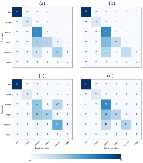
Figure 6.
Confusion matrix from inference analysis in Oregon from the (a) FC, (b) 1D-CNN, (c) 2D-CNN, and (d) 3D-CNN approaches.
Furthermore, in the case of the 2D-CNN, a higher degree of confusion is observed in the burned class, with approximately 50% of the labeled pixels being misclassified as bare soil. Furthermore, in the case of the 2D-CNN, approximately 50% of the labeled pixels in the burned class are misclassified as bare soil, while for the other models, the opposite pattern is observed. That is, a higher degree of confusion occurs in the bare soil class, where around 50% of the labeled pixels are misclassified as burned.
4.2. Statistical Comparison: p-value and T-Statistic
The statistical analysis utilized the “stats.ttest_ind” function from the “SciPy” library, enabling a comparison of performance metrics between different pairs of networks, and it was performed on the training dataset, and checked on the test dataset. Table 4 and Table 5 present the p-values and t-statistics obtained from the pairwise comparisons of F1 scores between different network pairs on the test dataset:
Table 4.
p-Value analysis for F1 score.
Table 5.
T-Statistic analysis for F1 score.
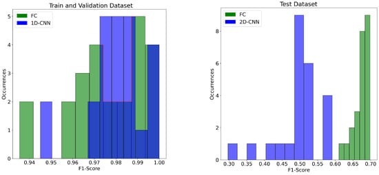
- p-value: at the top of Table 4, the p-values of , and indicate highly statistically significant differences in F1 scores between the FC network and the 2D-CNN and 3D-CNN networks, respectively. Conversely, the p-value of 0.5 for the comparison between the FC and 1D-CNN networks indicates no statistically significant difference in F1 scores between these models. This suggests that the FC architecture has similar performance to the 1D-CNN model but not to the 2D-CNN and 3D-CNN models in terms of F1 scores. The bottom of Table 4 reveals important insights into the performance differences among the neural network architectures on the Oregon dataset. The FC and 1D-CNN models exhibit slightly similar F1 scores, as indicated by the p-value of 0.19 in their comparison. On the other hand, the p-values of and suggest highly statistically significant differences between the FC and 2D-CNN, as well as the FC and 3D-CNN, respectively. Similarly, the other p-values, , and for the comparisons between the 1D-CNN and the 2D-CNN, the 1D-CNN and the 3D-CNN, and the 2D-CNN and the 3D-CNN networks indicate a statistically significant difference in F1 scores between these models. Thus, while the FC and 1D-CNN models exhibit similar performance, all of the other combinations show significant performance differences.
- T-Statistic: at the top of Table 5, it becomes evident that all of the observed values are relatively small. The t-statistic values, ranging from 1.50 to 2.81, indicating that the observed differences between the networks’ F1 scores are not large enough to assert a clear superiority of any specific network confidently. In contrast, the results derived from the evaluation of the Oregon dataset offer interesting and noteworthy insights (see the table located at the bottom of Table 5). In particular, a profound revelation emerges, indicating the clear underperformance of the 2D architecture when pitted against its counterparts. Indeed, the 2D architecture suffers a defeat in each pairwise challenge, revealing its inherent limitations compared to the other neural network architectures considered in this study.
The results from both analyses indicate significant performance differences between the different network pairs, suggesting that each model exhibits distinct strengths and weaknesses when evaluated on the specific datasets and geographical contexts. This observation is clearly depicted in Figure 7, where the two extreme cases (marked in bold in Table 4) are reported. The histograms visually illustrate that the case FC vs. 1D-CNN, on the left side, shows a significant overlap of data points, while the case FC vs. 2D-CNN, on the right side, displays complete separation between the data points. Especially, on the left side of Figure 7, a darker shade of blue was employed to clearly demarcate the regions where the two distributions overlap. Additionally, a thin red line traces the contour of the FC distribution to emphasize its underlying trend.
4.3. Inference Time and Model Complexity
In Table 6, the training time, the inference time, and the number of parameters are reported. All of the models demonstrate rapid training times on a range between 10 and 40 s. Moreover, the inference times for all models are impressively low, with values in a range between 0.3 and 0.6 ms. The number of parameters is also of the same order of magnitude. The results in Table 6 show valuable insights into the delicate balance between performance and computational complexity. Indeed, selecting an appropriate model depends on the application’s specific requirements. For instance, the FC model demonstrates impressive computational speed, as evidenced by its relatively short training (about 10 s) and inference times (about 0.3 ms) compared to the other models. Despite being the most computationally heavy with the highest number of parameters, the FC model’s efficient training and inference times indicate its capability to process data quickly and make predictions in a timely manner.
Table 6.
Training time, inference time and parameters for each model.
4.4. Additional Consideration from Visual/Manual Inspection
Given the scarcity of available pixels, a visual inspection of the segmentation and manual spectral analysis of specific pixels of interest, like large fire clusters, can provide further valuable results and insights into the various models. Unfortunately, the absence of a definitive ground truth map is a consequence of the unpredictable nature of wildfires. This inherent challenge underscores the necessity for in-depth research to develop models capable of generating such maps. This is the primary reason why this study has been undertaken—to address this critical need.
In this section, a representative case of training and test results of each model is selected and for each area of interest, the segmentation results over the entire PRISMA image are reported. Following this, a rigorous manual and visual inspection of the spectral data is conducted. The primary objective in this phase is to extract overarching insights from each segmentation within the different regions under investigation, with a specific emphasis on the analysis of macro zones associated with each class. During this detailed inspection, instances are revealed where certain macrozones do not authentically represent the underlying data.
4.4.1. Australia
While conducting a visual inspection of the Australian dataset, no additional significant findings emerged. This outcome, in line with the numerical results obtained across various datasets, underscores the consistency and reliability of our model’s performance. It is important to note that a substantial portion of our model’s training data originates from Australia. Consequently, the similarity in predictions between this region and others comes as no surprise. However, one can notice that the 3D model’s results offer a smoother, lower-noise image compared to the other models (refer to Figure 8 for visual comparison). This notable improvement can be attributed to the intricacies of the training process. Unlike the other models, the 3D model takes into account the spectral information of the surrounding area for each labeled pixel, rather than solely relying on the pixel’s own spectrum.
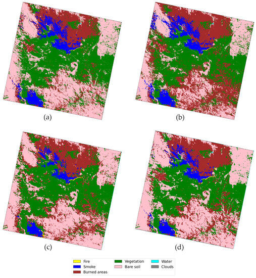
Figure 8.
Segmentation results in Australia from the (a) FC, (b) 1D-CNN, (c) 2D-CNN, and (d) 3D-CNN approaches.
4.4.2. Oregon
Figure 9 shows the results of transfer learning conducted in Oregon, presenting the predictions of the overall region for each analyzed model. Notably, the differences discussed in the confusion matrix are clearly evident. Moreover, the results obtained seem to suggest the presence of a significant active fire in Oregon, indicated by the black boxes in Figure 9, which the 3D model would not be able to detect. However, a thorough manual inspection reveals that no actual wildfire exists in those regions. Instead, the yellow pixels under consideration were manually classified as burnt areas, which is the same class correctly identified by the 3D model. This result underscores the potential advantages of the 3D model in real-world applications, as it demonstrates greater robustness in recognizing spatial patterns by incorporating contextual information from the surrounding areas.
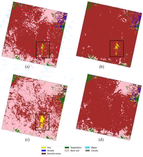
Figure 9.
Segmentation results in Oregon from the (a) FC, (b) 1D-CNN, (c) 2D-CNN, and (d) 3D-CNN approaches.
4.4.3. Sicily
The results of domain adaptation in Sicily are presented in Figure 10. It can be observed that all models accurately identify the burned areas in the upper right of the image, as well as successfully detect the three small pastoral fires. However, a notable discrepancy arises in the FC and 1D-CNN models, where a higher number of pixels are mislabeled as smoke in comparison to the 2D and 3D networks. In this context, the 2D and 3D CNN models demonstrate superior performance in image classification compared to the FC and 1D models, although they still face challenges in distinguishing smoke from shadows. This issue is more prominent in the 2D and 3D models. The underlying cause is the model’s limited ability to recognize shadows, which leads to confusion with the smoke spectrum, the closest known spectrum in this scenario. Furthermore, similar to the observations made in Oregon, all models except the 3D-CNN exhibit a tendency to detect relatively large fires near the burned areas, which do not actually exist. As a result, the 3D-CNN model emerges as the most reliable in accurately discerning real wildfires from false positives. Its advantage lies in its capability to recognize complex spatial features, especially in differentiating between the burned and fire classes where confusion is most prevalent. In conclusion, the 2D and 3D models, which integrate spatial information, demonstrate improved performance in smoothing and denoising image classifications.
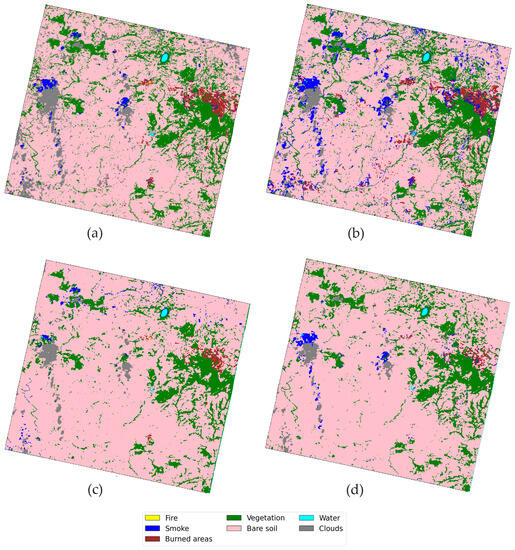
Figure 10.
Segmentation results in Sicily from the (a) FC, (b) 1D-CNN, (c) 2D-CNN, and (d) 3D-CNN approaches.
5. Discussion
This research was driven by the need to better manage wildfire events, as modern machine learning tools and hyperspectral imagery can provide useful information during and after the disaster. Considering the potentialities of PRISMA hyperspectral imagery, this study compared the results coming from different neural networks; the first two models (FC and 1D-CNN) are designed exclusively for spectral analysis, while the second two models (2D and 3D-CNN) are specifically tailored for conducting combined spatial and spectral analysis. The dataset is collected by manual inspection. Especially, the training and validation datasets are composed of the pixels from Australia, and the water and cloud classes in Sicily, while the test dataset is composed of the pixels from Oregon and the fire class from Sicily. Concerning the training of the four models, it was noted that the performances evaluated with the K-fold cross-validation were quite similar for the different approaches. Indeed, accuracies in the training dataset and test datasets were almost the same. Cross-validation was used to evaluate model performance and assess generalization capabilities. The results indicated stable and comparable performance across different cross-validation rounds for all neural network architectures, even if the FC results were slightly better.
The study conducted pairwise comparisons between neural network architectures using the p-value and t-statistic. The analysis conducted on both the training dataset and the test dataset revealed statistically significant differences in model performance, indicating that each architecture exhibited distinct strengths and weaknesses on the specific datasets and geographical contexts, except for FC and 1D-CNN. From the t-statistic, the FC model is recognized as the best model.
The study also analyzed the computational efficiency of each model, including training time, inference time, and the number of parameters. All models demonstrated very high computational speed, making them suitable for applications requiring quick processing and predictions, having a similar number of parameters. This is a very interesting outcome from an operational point of view, as all of the proposed methodologies could be used to assist ground operations and other management and detection operations.
When considering the classification ability for each class, smoke and burned soil pixels are well recognized by all models both in Australia and in Oregon. Referring to Figure 6, all of the models tend to confuse the other classes in the Oregon test case. Notably, the confusion matrices in Figure 6 only relate to a reduced subset of pixels from the Oregon area of interest and a visual inspection of the segmentation maps can provide additional valuable details.
Furthermore, visual and manual spectrum inspections of the classification maps are conducted. These inspections suggests that the 3D-CNN model outperformed the others in recognizing spatial patterns and exhibited better performance in distinguishing between burned areas and false positives. Indeed, the 2D and the 3D models provide the most clear and less-noisy maps, due to their ability to mix spectral and spatial information. However, the 3D model seems to be the only one to avoid important false alarms, unlike the other models, which detect a fire that was not actually present, as is clearly shown in the zoomed areas on the right of Figure 9. Moreover, similar conclusions are obtained in Sicily, where the graphical inspection of the segmentation maps reported in Figure 10 demonstrates that a large number of pixels were misclassified as smoke by the 1D model. The results from the 3D model show that the shadows from the clouds were classified as smoke. Nonetheless, this error can be accepted as the class ’shadow’ and was not considered in the set of input labels. To sum up, the numerical results seem to confirm a slight superiority of the fully connected model, but the visual/manual inspection of the segmentation maps reveals that those from the 3D models are less noisy than the ones provided by the other models.
This specific aspect deserves further investigation for future work. Notably, an ensemble of the proposed models could be proposed for further investigation, as it could merge the benefits from each singular model.
The network’s intrinsic limitation lies in its reliance on a restricted amount of input data. Indeed, this limitation is inherent to the field of fire detection, where the availability of reliable ground truth maps is inherently scarce. This scarcity of ground truth data underscores the significant and ongoing interest in this field, as researchers strive to address this fundamental challenge. Moreover, the results underscore a noticeable performance gap between the training dataset and the test dataset, with an approximate 20% reduction in performance. While this divergence does raise valid concerns about potential overfitting, it is vital to acknowledge the substantial environmental diversity across Australia, Sicily, and Oregon. These environmental variations are reasonable factors contributing to the observed performance differences. Therefore, it is essential to interpret these findings while keeping in mind the limitations of the available data points and the impact of environmental diversity. Further investigations and additional data collection may be required to conclusively determine the presence and extent of overfitting.
Despite its high precision in detecting fire, smoke, and scorched earth with the aid of low-noise signal PRISMA datum, the network becomes confused when shadows are present and may classify them as smoke. Moreover, the confusion matrices in Figure 6 based on the small set of labeled points in Oregon show that apart from fire and smoke, the other classes can be confused in new scenarios. Therefore, to increase the CNN performance for future works, the CNN training dataset should be increased, and this operation can be conducted both manually (which is a time-consuming activity that generates high-reliability results) or automatically (which is a fast operation that can generate a noisy input dataset). In the latter case, the training dataset could be increased by using together Jeffries Matusita (JM) and Spectral Angle Mapper (SAM) distances between two spectra that compute spectral similarity, as reported in [50,51,52]. In this way, it would be possible to insert in each class similar spectrum signals by scanning the entire hypercube data from PRISMA. To improve the model’s ability to distinguish shadows from clouds, it is crucial to add new classes, thus obtaining a more sophisticated neural network capable of performing more precise analyses. Simply following the aforementioned steps may not be sufficient in all cases. In some cases, errors may arise due to the fact that individual pixels are composites of several signals, such as with smoke, causing confusion within the neural network system. To mitigate this issue, a potential solution could be the implementation of a CNN for an unmixing analysis. In this case, the input dataset should report the percentage of each class in each pixel instead of the majority class. This analysis will be considered in future works for the improvement of the current results.
6. Conclusions
Satellite-based data processing is an essential asset in disaster management, especially in wildfires, offering valuable information for both pre-fire strategic planning and post-fire recovery efforts. Using satellite data can enhance our comprehension and control of these complex and ever-changing phenomena, reducing the adverse impacts and human casualties associated with wildfires. The research conducted in the present investigation primarily aimed to identify wildfires through the utilization of hyperspectral imagery obtained from the PRISMA satellite. This was achieved by employing artificial neural networks (ANNs), with a specific focus on convolutional neural networks (CNNs). The current research presents findings on segmentation studies employing a fully connected (FC) network and three different CNN architectures (one-dimensional, two-dimensional, and three-dimensional models, also referred to as 1D, 2D, and 3D models) testing the generalization ability through domain adaption. Based on the findings presented, it appears that the fully connected model achieves top performances in classification abilities, even though the models based on a spatial-spectral analysis provide smother and less-noisy maps. More specifically, the classification maps indicate that the 3D model exhibits a greater capacity to avoid false alarms compared to the other models. This result unequivocally supports prioritizing the development of the 3D model. While the findings may not conclusively establish it as the superior solution, the lower false alarm rate observed with the 3D model suggests its potential for further investigation and refinement. This direction presents a promising avenue for future research and development in the context of wildfire detection.
Overall, the proposed methodologies have the potential to offer significant assistance in complementing other assessments performed on the ground for the purposes of wildfire identification and management. The Oregon test dataset demonstrates effective detection of fire and smoke classes. As an example, the fire class is categorized with a perfect F1 score of 100%, according to the FC and 1D model. Nevertheless, it is worth noting that all models exhibit a tendency to misclassify other classes regularly and are prone to generating false alarms. Future research endeavors could potentially enhance the findings of this study by incorporating larger training datasets and employing more complex neural networks that possess the ability to do unmixing research studies.
Author Contributions
Conceptualization: D.S., S.A. and K.T.; methodology: D.S.; software: D.S.; validation: A.C.; formal analysis: A.C.; investigation: D.S. and A.C.; resources: R.S. and G.L.; writing—original draft preparation: A.C., K.T. and S.A.; writing—review and editing: D.S.; visualization: D.S., A.C. and K.T.; supervision: R.S. and G.L. All authors have read and agreed to the published version of the manuscript.
Funding
The authors would like to thank Khalifa University and the SmartSat Cooperative Research Centre (CRC) for their partial support of this work through Grant No. FSU-2022-013 and the Doctoral Research Project No. 2.13s respectively.
Data Availability Statement
The code and data are available at: https://github.com/DarioSpiller/Tutorial_PRISMA_IGARSS_wildfires (accessed on 14 July 2023).
Conflicts of Interest
The authors declare no conflict of interest.
Abbreviations
The following abbreviations are used in this manuscript:
| CNN | Convolutional Neural Networks |
| HS | Hyperspectral |
| PRISMA | PRecursore IperSpettrale della Missione Applicativa |
| SWIR | Short-Wave InfraRed |
| VNIR | Visible and Near InfraRed |
| ML | Machine Learning |
| HFDI | Hyperspectral Fire Detection Index |
References
- Lollino, G.; Manconi, A.; Guzzetti, F.; Culshaw, M.; Bobrowsky, P.; Luino, F. (Eds.) Remote Sensing Role in Emergency Mapping for Disaster Response; Springer International Publishing: Berlin, Germany, 2015. [Google Scholar] [CrossRef]
- Yang, J.; Gong, P.; Fu, R.; Zhang, M.; Chen, J.; Liang, S.; Xu, B.; Shi, J.; Dickinson, R. The role of satellite remote sensing in climate change studies. Nat. Clim. Chang. 2014, 4, 875–883, Erratum in Nat. Clim. Change 2014, 4, 74. [Google Scholar] [CrossRef]
- Chien, S.; Tanpipat, V. Remote Sensing of Natural Disasters; Springer: New York, NY, USA, 2012; pp. 8939–8952. [Google Scholar] [CrossRef]
- Mansoor, S.; Farooq, I.; Kachroo, M.M.; Mahmoud, A.E.D.; Fawzy, M.; Popescu, S.M.; Alyemeni, M.; Sonne, C.; Rinklebe, J.; Ahmad, P. Elevation in wildfire frequencies with respect to the climate change. J. Environ. Manag. 2022, 301, 113769. [Google Scholar] [CrossRef] [PubMed]
- Abram, N.; Henley, B.; Sen Gupta, A.; Lippmann, T.J.; Clarke, H.; Dowdy, A.J.; Sharples, J.J.; Nolan, R.H.; Zhang, T.; Wooster, M.J.; et al. Connections of climate change and variability to large and extreme forest fires in southeast Australia. Commun. Earth Environ. 2021, 2, 8. [Google Scholar] [CrossRef]
- Barmpoutis, P.; Papaioannou, P.; Dimitropoulos, K.; Grammalidis, N. A review on early forest fire detection systems using optical remote sensing. Sensors 2020, 20, 6442. [Google Scholar] [CrossRef] [PubMed]
- Bu, F.; Gharajeh, M.S. Intelligent and vision-based fire detection systems: A survey. Image Vis. Comput. 2019, 91, 103803. [Google Scholar] [CrossRef]
- Domenikiotis, C.; Loukas, A.; Dalezios, N.R. The use of NOAA/AVHRR satellite data for monitoring and assessment of forest fires and floods. Nat. Hazards Earth Syst. Sci. 2003, 3, 115–128. [Google Scholar] [CrossRef]
- Davies, D.; Ederer, G.; Olsina, O.; Wong, M.; Cechini, M.; Boller, R. NASA’s Fire Information for Resource Management System (FIRMS): Near Real-Time Global Fire Monitoring Using Data from MODIS and VIIRS. In Proceedings of the EARSeL Forest Fires SIG Workshop, Matera, Italy, 3–6 June 2020. [Google Scholar]
- Veraverbeke, S.; Dennison, P.; Gitas, I.; Hulley, G.; Kalashnikova, O.; Katagis, T.; Kuai, L.; Meng, R.; Roberts, D.; Stavros, N. Hyperspectral remote sensing of fire: State-of-the-art and future perspectives. Remote Sens. Environ. 2018, 216, 105–121. [Google Scholar] [CrossRef]
- Barducci, A.; Guzzi, D.; Marcoionni, P.; Pippi, I. Comparison of fire temperature retrieved from SWIR and TIR hyperspectral data. Infrared Phys. Technol. 2004, 46, 1–9. [Google Scholar] [CrossRef]
- Waigl, C.F.; Prakash, A.; Stuefer, M.; Verbyla, D.; Dennison, P. Fire detection and temperature retrieval using EO-1 Hyperion data over selected Alaskan boreal forest fires. Int. J. Appl. Earth Obs. Geoinf. 2019, 81, 72–84. [Google Scholar] [CrossRef]
- Amici, S.; Wooster, M.J.; Piscini, A. Multi-resolution spectral analysis of wildfire potassium emission signatures using laboratory, airborne and spaceborne remote sensing. Remote Sens. Environ. 2011, 115, 1811–1823. [Google Scholar] [CrossRef]
- Vodacek, A.; Kremens, R.L.; Fordham, A.J.; Vangorden, S.C.; Luisi, D.; Schott, J.R.; Latham, D.J. Remote optical detection of biomass burning using a potassium emission signature. Int. J. Remote Sens. 2002, 23, 2721–2726. [Google Scholar] [CrossRef]
- Griffin, M.K.; Hsu, S.M.; Burke, H.h.K.; Snow, J.W. Characterization and delineation of plumes, clouds and fires in hyperspectral images. In Proceedings of the International Geoscience and Remote Sensing Symposium (IGARSS), Honolulu, HI, USA, 24–28 July 2000. [Google Scholar] [CrossRef]
- Shaik, R.U.; Relangi, N.; Thangavel, K. Mathematical Modelling of a Propellent Gauging System: A Case Study on PRISMA. Aerospace 2023, 10, 567. [Google Scholar] [CrossRef]
- Gagliardi, V.; Tosti, F.; Bianchini Ciampoli, L.; Battagliere, M.L.; D’Amato, L.; Alani, A.M.; Benedetto, A. Satellite remote sensing and non-destructive testing methods for transport infrastructure monitoring: Advances, challenges and perspectives. Remote Sens. 2023, 15, 418. [Google Scholar] [CrossRef]
- Piano Nazionale di Ripresa e Resilienza (PNRR). Available online: https://www.governo.it/sites/governo.it/files/PNRR.pdf (accessed on 17 April 2023).
- Fang, L.; Yan, Y.; Yue, J.; Deng, Y. Toward the Vectorization of Hyperspectral Imagery. IEEE Trans. Geosci. Remote Sens. 2023, 61, 1–14. [Google Scholar] [CrossRef]
- Priego, B.; Duro, R.J. An Approach for the Customized High-Dimensional Segmentation of Remote Sensing Hyperspectral Images. Sensors 2019, 19, 2887. [Google Scholar] [CrossRef] [PubMed]
- Shaik, R.U.; Laneve, G.; Fusilli, L. An automatic procedure for forest fire fuel mapping using hyperspectral (PRISMA) imagery: A semi-supervised classification approach. Remote Sens. 2022, 14, 1264. [Google Scholar] [CrossRef]
- Singh, S.; Kasana, S.S. Spectral-Spatial Hyperspectral Image Classification using Deep Learning. In Proceedings of the 2019 Amity International Conference on Artificial Intelligence (AICAI), Dubai, United Arab Emirates, 4–6 February 2019; pp. 411–417. [Google Scholar] [CrossRef]
- Grewal, R.; Singh Kasana, S.; Kasana, G. Machine Learning and Deep Learning Techniques for Spectral Spatial Classification of Hyperspectral Images: A Comprehensive Survey. Electronics 2023, 12, 488. [Google Scholar] [CrossRef]
- Pattem, S.; Thatavarti, S. Hyperspectral Image Classification using Machine Learning Techniques—A Survey. In Proceedings of the 2023 IEEE International Students’ Conference on Electrical, Electronics and Computer Science (SCEECS), Bhopal, India, 18–19 February 2023; pp. 1–14. [Google Scholar] [CrossRef]
- Zhang, L.; Zhang, L. Artificial Intelligence for Remote Sensing Data Analysis: A review of challenges and opportunities. IEEE Geosci. Remote Sens. Mag. 2022, 10, 270–294. [Google Scholar] [CrossRef]
- Paoletti, M.; Haut, J.; Plaza, J.; Plaza, A. Deep learning classifiers for hyperspectral imaging: A review. ISPRS J. Photogramm. Remote Sens. 2019, 158, 279–317. [Google Scholar] [CrossRef]
- Petersson, H.; Gustafsson, D.; Bergstrom, D. Hyperspectral image analysis using deep learning—A review. In Proceedings of the 2016 Sixth International Conference on Image Processing Theory, Tools and Applications (IPTA), Oulu, Finland, 12–15 December 2016; pp. 1–6. [Google Scholar]
- Wang, C.; Liu, B.; Liu, L.; Zhu, Y.; Hou, J.; Liu, P.; Li, X. A review of deep learning used in the hyperspectral image analysis for agriculture. Artif. Intell. Rev. 2021, 54, 5205–5253. [Google Scholar] [CrossRef]
- Amici, S.; Spiller, D.; Ansalone, L.; Miller, L. Wildfires Temperature Estimation by Complementary Use of Hyperspectral PRISMA and Thermal (ECOSTRESS &L8). J. Geophys. Res. Biogeosci. 2022, 127, e2022JG007055. [Google Scholar] [CrossRef]
- Thangavel, K.; Spiller, D.; Sabatini, R.; Amici, S.; Longepe, N.; Servidia, P.; Marzocca, P.; Fayek, H.; Ansalone, L. Trusted Autonomous Operations of Distributed Satellite Systems Using Optical Sensors. Sensors 2023, 23, 3344. [Google Scholar] [CrossRef] [PubMed]
- Thangavel, K.; Spiller, D.; Sabatini, R.; Servidia, P.; Marzocca, P.; Fayek, H.M.; Khaja Faisal, H.; Gardi, A. Trusted Autonomous Distributed Satellite System Operations for Earth Observation. In Proceedings of the 17th International Conference on Space Operations, Dubai, United Arab Emirates, 6–10 March 2023. [Google Scholar] [CrossRef]
- Thangavel, K. Trusted Autonomous Operations of Distributed Satellite Systems for Earth Observation Missions. Ph.D. Thesis, RMIT University, Melbourne, Australia, 2023. [Google Scholar]
- Miralles, P.; Thangavel, K.; Scannapieco, A.F.; Jagadam, N.; Baranwal, P.; Faldu, B.; Abhang, R.; Bhatia, S.; Bonnart, S.; Bhatnagar, I.; et al. A critical review on the state-of-the-art and future prospects of Machine Learning for Earth Observation Operations. Adv. Space Res. 2023, 71, 4959–4986. [Google Scholar] [CrossRef]
- Ranasinghe, K.; Sabatini, R.; Gardi, A.; Bijjahalli, S.; Kapoor, R.; Fahey, T.; Thangavel, K. Advances in Integrated System Health Management for mission-essential and safety-critical aerospace applications. Prog. Aerosp. Sci. 2022, 128, 100758. [Google Scholar] [CrossRef]
- Thangavel, K.; Spiller, D.; Sabatini, R.; Amici, S.; Sasidharan, S.T.; Fayek, H.; Marzocca, P. Autonomous Satellite Wildfire Detection Using Hyperspectral Imagery and Neural Networks: A Case Study on Australian Wildfire. Remote Sens. 2023, 15, 720. [Google Scholar] [CrossRef]
- Spiller, D.; Thangavel, K.; Sasidharan, S.T.; Amici, S.; Ansalone, L.; Sabatini, R. Wildfire segmentation analysis from edge computing for on-board real-time alerts using hyperspectral imagery. In Proceedings of the 2022 IEEE International Conference on Metrology for Extended Reality, Artificial Intelligence and Neural Engineering (MetroXRAINE), Rome, Italy, 26–28 October 2022; pp. 725–730. [Google Scholar] [CrossRef]
- Thangavel, K.; Spiller, D.; Sabatini, R.; Marzocca, P. On-board Data Processing of Earth Observation Data Using 1-D CNN. In Proceedings of the SmartSat CRC Conference, Sydey, Australia, 12–13 September 2022. [Google Scholar] [CrossRef]
- Thangavel, K.; Servidia, P.; Sabatini, R.; Marzocca, P.; Fayek, H.; Cerruti, S.H.; España, M.; Spiller, D. A Distributed Satellite System for Multibaseline AT-InSAR: Constellation of Formations for Maritime Domain Awareness Using Autonomous Orbit Control. Aerospace 2023, 10, 176. [Google Scholar] [CrossRef]
- Thangavel, K.; Spiller, D.; Sabatini, R.; Marzocca, P.; Esposito, M. Near Real-time Wildfire Management Using Distributed Satellite System. IEEE Geosci. Remote Sens. Lett. 2022, 20, 1–5. [Google Scholar] [CrossRef]
- Thangavel, K.; Servidia, P.; Sabatini, R.; Marzocca, P.; Fayek, H.; Spiller, D. Distributed Satellite System for Maritime Domain Awareness. In Proceedings of the Australian International Aerospace Congress (AIAC20), Melbourne, Australia, 27–28 February 2023; pp. 27–28. [Google Scholar]
- Guarini, R.; Loizzo, R.; Facchinetti, C.; Longo, F.; Ponticelli, B.; Faraci, M.; Dami, M.; Cosi, M.; Amoruso, L.; De Pasquale, V.; et al. PRISMA hyperspectral mission products. In Proceedings of the International Geoscience and Remote Sensing Symposium (IGARSS), Valencia, Spain, 22–17 July 2018. [Google Scholar] [CrossRef]
- Centre, J.; San-Miguel-Ayanz, J.; Durrant, T.; Boca, R.; Maianti, P.; Libertà, G.; Artés Vivancos, T.; Oom, D.; Branco, A. Forest Fires in Europe, Middle East and North Africa 2021; Publications Office of the European Union: Luxembourg, 2022. [Google Scholar] [CrossRef]
- Amici, S.; Piscini, A. Exploring prisma scene for fire detection: Case study of 2019 bushfires in ben halls gap national park, nsw, australia. Remote Sens. 2021, 13, 1410. [Google Scholar] [CrossRef]
- Spiller, D.; Ansalone, L.; Amici, S.; Piscini, A.; Mathieu, P. Analysis and detection of wildfires by using prisma hyperspectral imagery. Int. Arch. Photogramm. Remote Sens. Spat. Inf. Sci. 2021, 43, 215–222. [Google Scholar] [CrossRef]
- Hu, W.; Huang, Y.; Wei, L.; Zhang, F.; Li, H. Deep convolutional neural networks for hyperspectral image classification. J. Sensors 2015, 2015, 258619. [Google Scholar] [CrossRef]
- Xi, Y.; Ren, C.; Wang, Z.; Wei, S.; Bai, J.; Zhang, B.; Xiang, H.; Chen, L. Mapping Tree Species Composition Using OHS-1 Hyperspectral Data and Deep Learning Algorithms in Changbai Mountains, Northeast China. Forest 2019, 10, 8181. [Google Scholar] [CrossRef]
- Spiller, D.; Amici, S.; Ansalone, L. Transfer Learning Analysis For Wildfire Segmentation Using Prisma Hyperspectral Imagery And Convolutional Neural Networks. In Proceedings of the 2022 12th Workshop on Hyperspectral Imaging and Signal Processing: Evolution in Remote Sensing (WHISPERS), Rome, Italy, 13–16 September 2022; pp. 1–5. [Google Scholar] [CrossRef]
- Hastie, T.; Tibshirani, R.; Friedman, J.H.; Friedman, J.H. The Elements of Statistical Learning: Data Mining, Inference, and Prediction; Springer: Berlin, Germany, 2009; Volume 2. [Google Scholar]
- Kramer, O. Scikit-learn. In Machine Learning for Evolution Strategies; Springer: Berlin, Germany, 2016; pp. 45–53. [Google Scholar]
- Padma, S.; Sanjeevi, S. Jeffries Matusita based mixed-measure for improved spectral matching in hyperspectral image analysis. Int. J. Appl. Earth Obs. Geoinf. 2014, 32, 138–151. [Google Scholar] [CrossRef]
- Padma, S.; Sanjeevi, S. Jeffries Matusita-Spectral Angle Mapper (JM-SAM) spectral matching for species level mapping at Bhitarkanika, Muthupet and Pichavaram mangroves. Int. Arch. Photogramm. Remote Sens. Spat. Inf. Sci. 2014, 40, 1403. [Google Scholar] [CrossRef]
- Bruzzone, L.; Roli, F.; Serpico, S. An extension of the Jeffreys-Matusita distance to multiclass cases for feature selection. IEEE Trans. Geosci. Remote Sens. 1995, 33, 1318–1321. [Google Scholar] [CrossRef]
Disclaimer/Publisher’s Note: The statements, opinions and data contained in all publications are solely those of the individual author(s) and contributor(s) and not of MDPI and/or the editor(s). MDPI and/or the editor(s) disclaim responsibility for any injury to people or property resulting from any ideas, methods, instructions or products referred to in the content. |
© 2023 by the authors. Licensee MDPI, Basel, Switzerland. This article is an open access article distributed under the terms and conditions of the Creative Commons Attribution (CC BY) license (https://creativecommons.org/licenses/by/4.0/).