Article

Evaluating Close-Range Photogrammetry for 3D Understory Fuel Characterization and Biomass Prediction in Pine Forests

1
School of Environmental and Forest Sciences, University of Washington, Seattle, WA 98195, USA
2
Desert Research Institute, Reno, NV 89512, USA
3
Division of Sciences and Mathematics, School of Interdisciplinary Arts and Sciences, University of Washington, Tacoma, WA 98402, USA
*
Author to whom correspondence should be addressed.
Remote Sens. 2023, 15(19), 4837; https://doi.org/10.3390/rs15194837
Submission received: 26 July 2023 / Revised: 26 September 2023 / Accepted: 4 October 2023 / Published: 6 October 2023
(This article belongs to the Section Forest Remote Sensing)

Abstract

:
Understory biomass plays an important role in forests, and explicit characterizations of live and dead understory vegetation are critical for wildland fuel characterization and to link understory vegetation to ecosystem processes. Current methods to accurately model understory fuel complexity in 3D rely on expensive and often inaccessible technologies. Structure-from-motion close-range photogrammetry, in which ordinary photographs or video stills are overlaid to generate point clouds, is promising as an alternative method to generate 3D models of fuels at a fraction of the cost of more traditional field surveys. In this study, we compared the performance of close-range photogrammetry with field sampling surveys to assess the utility of this alternative technique for quantifying understory fuel structure. Using a commercially available GoPro camera, we generated 3D point cloud models from video-derived image stills of 138 sampling plots across two western ponderosa pine and two southeastern slash pine sites. We directly compared structural metrics derived from the photogrammetry to those derived from field sampling, then evaluated predictive models of biomass calibrated by means of destructive sampling. Photogrammetry-derived measures of occupied volume and fuel height showed strong agreements with field sampling (Pearson’s R = 0.81 and 0.86, respectively). While we found weak relationships between photogrammetry metrics and biomass 0 to 10 cm in height, occupied volume and a novel metric to characterize the vertical profile of vegetation produced the strongest relationships with biomass above the litter layer (i.e., >10 cm) across different fuel types (R2 = 0.55–0.76). The application of this technique has the potential to provide managers with an accessible option for inexpensive data collection and can lay the groundwork for the rapid collection of input datasets to train landscape-scale fuel models.

1. Introduction

The amount and structure of understory biomass play an integral role in forest ecosystem processes. Configurations of live and dead understory vegetation provide forage and habitat for wildlife, directly influencing species richness and survivorship [1,2]. Vegetation cover and litter are important aspects of soil nutrient cycling and mitigate erosion potential [3,4]. Live understory vegetation can account for a large portion of the carbon and nitrogen fluxes in forests and is considered an overall indicator of forest health [5,6]. Understory biomass is also a critical source of fuel in wildland fires, and its arrangement in both horizontal and vertical space influences patterns of fire spread, consumption, and fire severity impacts on vegetation and soils [7,8,9]. Vegetation height and vertical continuity govern the probability of a transition from ground to crown fire, and fuels below the canopy are the primary driver of combustion in forests with high-frequency, low-intensity fire regimes [10,11]. Spatially explicit three-dimensional (3D) characterizations of understory biomass are instrumental in linking vegetation to ecosystem processes, but capturing their complexity at scales relevant to forest managers remains a challenge [12].
Traditionally, assessments of understory fuel structure to quantify biomass have been conducted in-field through visual estimation [13] or the use of point-intercept or transect sampling, which can be time consuming and error prone [12,14]. Although these methods have proven useful for coarse-grain estimations and modeling, they are abstractions of fuel conditions and largely fail to capture the fine-scale heterogeneity required for 3D fuel inputs in computational fluid dynamics modeling of fire behavior [7,8]. As such, the development of more accessible, efficient, and reliable methods to characterize fine-scale fuel structure and quantify biomass is needed.
Satellite and airborne remote sensing methods—including airborne lidar, unoccupied aerial surveys (UAS), and UAS-derived photogrammetry—have been used extensively to quantify canopy fuels in 3D but are largely insufficient for understory fuel characterization due to canopy obstruction and inadequate spatial resolution [15,16]. Ground-based remote sensing methods such as terrestrial lidar scanning (TLS) have demonstrated reliability in capturing understory fuel structure and have been used to quantify vegetation structure, biomass, and leaf area with high accuracy [9,17,18,19,20]. Despite this reliability and precision, TLS scanning instruments have a high cost, can be laborious to apply, and survey-grade instruments can be difficult to maneuver in rough or remote terrain [16,19].
Structure-from-motion (SfM) photogrammetry, in which overlapping images are arranged to create a 3D point cloud, has shown promise as an accessible alternative to field-based sampling and more expensive ground-based remote sensing techniques. Simple summary metrics of SfM point clouds such as height and occupied volume derived from voxelization have been used to quantify the 3D structure of fuels such as grasses, shrubs, fine woody debris, and tree diameter in previous studies with moderate accuracy [21,22,23,24]. As an emerging approach for forest inventory analysis, previous methods used to generate SfM point clouds have relied on the collection of dozens of still photographs taken individually by a camera from multiple viewpoints at consistent distances over several minutes. While this approach provides an advancement over more time-consuming, traditional field-based sampling, evaluation and refinements to the SfM data collection technique itself to streamline data collection are warranted.
To advance close-range photogrammetry from its current status as a novel alternative to a reliable remote sensing technique, refinements to the SfM data collection and evaluation of its utility to characterize biomass are needed. SfM point clouds generated from short videos rather than the individual photographs that have dominated previous studies can resolve known issues that may arise if an insufficient or inconsistent number of photos are taken in the field [24], as well as reduce the time and effort required for data collection. Videos recorded with affordable handheld cameras can be easily parsed into hundreds of still images by means of automated scripts for use in photogrammetry processing software to build point cloud models. Computational advancements in photogrammetric software and refined data processing methods have enormous potential to lay the groundwork for fully automated workflows to produce 3D point clouds that can be used for operational mapping and machine learning algorithms to model surface fuel configurations across landscapes.
The purpose of this study was to evaluate a novel data collection technique for generating close-range photogrammetric point clouds for understory fuel characterization in 3D. We generated a dataset of 138 video-derived photogrammetry models, paired them with a voxel-based field inventory and destructive sampling plots, and from them calculated a suite of summary metrics to test their ability to predict understory biomass. We integrated metrics commonly used in previous assessments of close-range photogrammetry, as well as a novel metric to characterize the vertical profile of vegetation introduced in this study. Datasets were collected from four sites across two contrasting systems in the United States: southeastern slash pine and western ponderosa pine forests. Though our sites had similar overstory characteristics, they had a markedly different understory structure and composition, providing an opportunity to test our method and metrics across different fuel complexes and forest types. Our study addressed the following research questions: (1) how well do photogrammetric point clouds characterize fuel structure compared to field sampling? (2) Can measures of fuel structure from photogrammetric point clouds be used to develop predictive models of biomass? (3) How generalizable are these models across different fuel complexes and forest types?

2. Materials and Methods

2.1. Study Area

Datasets were collected between July 2019 and February 2020 from four sites across the United States: Lubrecht Experimental Forest in Montana, Sycan Marsh Preserve in Oregon, and two sites at Tate’s Hell State Forest in Florida (Figure 1). These sites were selected to capture the broad range of understory fuel structure and composition across sites with similar overstory characteristics and are characterized by open forest canopies with minimal canopy layering and ladder fuels. All four sites were prescribed burned in the past, with a range of times since last fire.

2.1.1. Lubrecht Experimental Forest

Lubrecht Experimental Forest (LUB) is located approximately 30 miles east of Missoula in the Blackfoot River drainage of western Montana. The overstory at LUB consists of predominantly ponderosa pine (Pinus ponderosa) and Douglas fir (Pseudotsuga menziesii), with sparse understory vegetation dominated by scattered shrubs (Vaccinium spp.), kinnikinnick (Arctostaphylos uva-ursi), and timber litter. The site was mechanically thinned during the winter of 2001, and last burned in the late spring of 2002. Sampling was conducted at LUB in July 2019.

2.1.2. Sycan Marsh Preserve—Forest

Situated in the Klamath Basin of southern Oregon, Sycan Marsh Preserve spans over 12,000 hectares of mostly marsh and grassland, with an upland forest area where sampling for this study took place in September and October 2019. The forested site at the preserve (SMF) consists of open-canopy and uneven-aged ponderosa pine forest, with evidence of past logging and thinning. The understory vegetation at SMF is dominated by scattered bitterbrush (Purshia tridentata) with some bunchgrasses, and surface fuels include fine wood (10 h and 100 h) with occasional rotten coarse woody debris. The site was thinned using an individual, clump, and openings prescription [25] in 2019 and prescribed burned immediately following our sampling campaign.

2.1.3. Tate’s Hell State Forest

We established two separate sampling sites at Tate’s Hell State Forest, located in the central panhandle of northern Florida. The first site, referred to as Tate’s Hell A (THA), was sampled in late January 2020 and is located in a mesic flatwood forest that was burned approximately one year prior to sampling. The overstory is dominated by open canopy slash pine (P. elliottii), and the understory is dominated by saw palmetto (Serenoa repens) and gallberry (Ilex glabra), with some deciduous shrubs, oak seedlings, and grasses present in smaller abundance. The second site, referred to as Tate’s Hell B (THB) and sampled in early February 2020, is similarly located in a mesic flatwood forest dominated by open canopy slash pine, but was burned between two and three years previously. As a result, the understory of THB contained similar species to THA (dominated by saw palmetto and gallberry), but with greater height and density.

2.2. Sampling Design and Processing

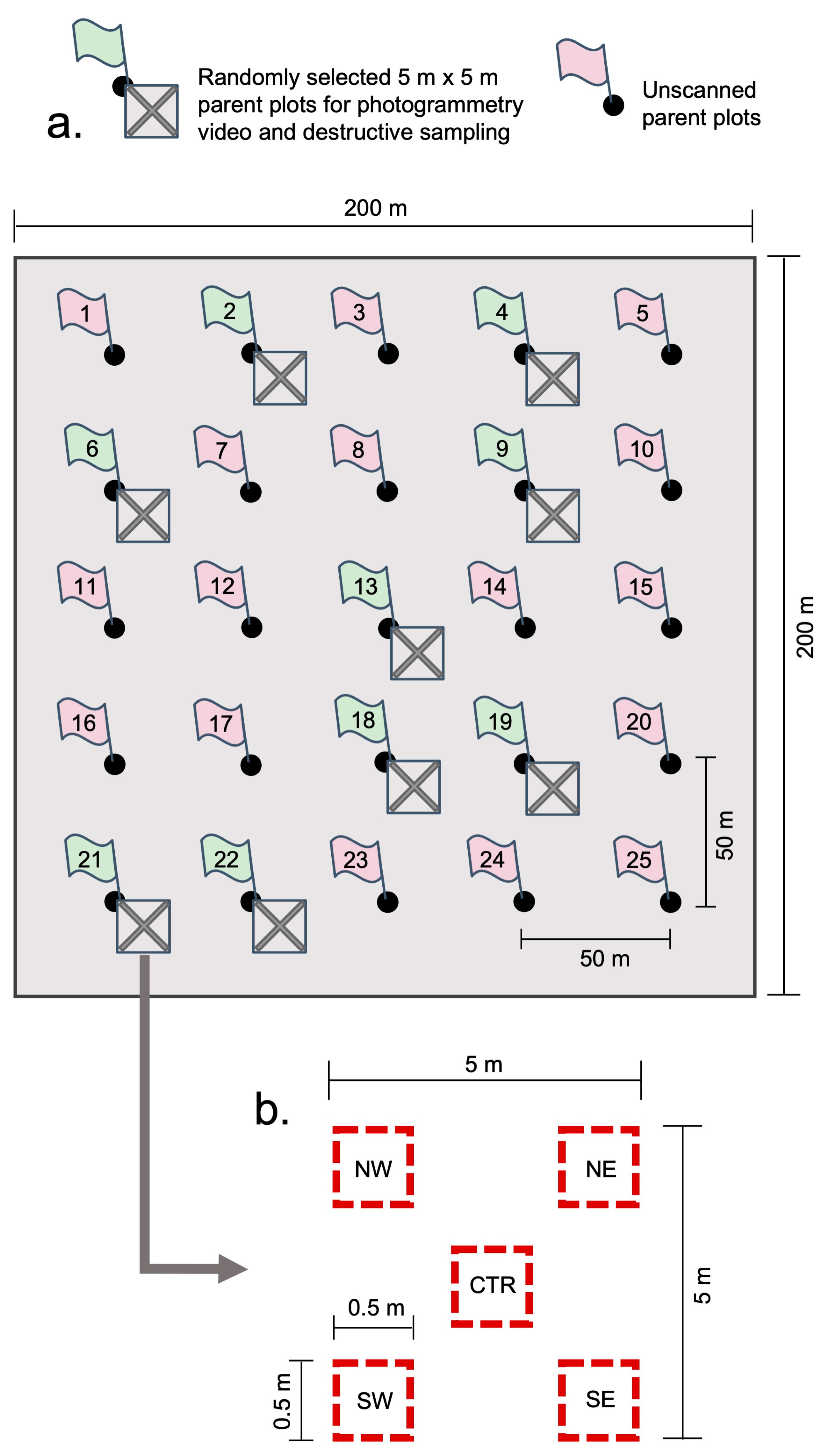
Within each of the four sites, photogrammetry and field sampling areas were selected that had relatively open forest canopies (less than 50% canopy closure), gradual slope gradients (less than 20%), and were located within a consistent management history of past thinning and burning across the site. At each site, a 40,000 m2 sampling area was identified and divided into a grid of 25 parent plots spanning 5 by 5 m, spaced roughly 50 m apart (Figure 2a). Of the 25 parent plots, nine were randomly selected for destructive sampling at each site. In each of the randomly selected parent plots, five individual 0.5 by 0.5 m voxel sampling plots (hereinafter, plots) delineated by reflective red and white PVC pipe frames were established in an “X” formation, with one plot at each of the northwest, northeast, southwest, and southeast corners of the cell and one plot positioned at the center (Figure 2b). At each of the plots, we conducted close-range scanning, a field inventory, and destructive sampling. In total, 45 plots were sampled at LUB, THA, and THB, and 16 plots were sampled at SMF (total n = 151 plots). The SMF site was part of a separate prescribed burn study, and a portion of the plots (n = 29) were reserved for post-burn sampling and scanning; they were therefore not included in this study.

2.2.1. Close-Range Photogrammetry

Close-range scanning of each plot was conducted using a GoPro HERO7 Black camera mounted to a monopod. To obtain consistent scans across all 151 plots, the camera was held at a constant nadir angle and video was recorded using a side-to-side, slow sweeping motion 1 to 1.5 m above the ground at each plot. We positioned the camera so that the red and white PVC sampling frames remained fully visible throughout each video, as these frames were later used in post-processing as tie points to build the final photogrammetric point clouds. Videos were acquired in the morning (9 a.m. to 11 a.m. local time) at each site and took from 30 s to a minute and a half per plot. All videos were exported and saved as MP4 files.
Point cloud models were produced from each video (Figure S1 within the Supplementary Materials) using a combination of Python scripts and Agisoft Metashape Pro version 1.7.2 (https://www.agisoft.com/, accessed on 25 March 2021). Agisoft is a commercial software tool specifically for photogrammetry creation and analysis; it incorporates machine learning techniques to pair sequential images of discrete objects taken from multiple angles to generate stereo or 3D models. Because of this, past studies assessing close-range photogrammetry have typically used individual photographs to generate their 3D models [21,22,23,24]. While our method of collecting short videos from the GoPro camera increases the speed of data collection (30 s versus several minutes for some studies [24]), individual images are still necessary in the Agisoft workflow. To produce these images from our videos, we implemented a pre-processing step in Python to parse each MP4 video file into approximately 400 still images. The Python script included an additional step to filter out the very first and very last few scenes of each video, which often contained shaky views of non-vegetation (i.e., the sky or field equipment) as field technicians started and stopped recording on the device. The final images, saved as individual image files (.PNG), were then imported into Agisoft for processing.
As part of the workflow to produce a 3D model, Agisoft first automatically searches for common points on every image provided to the software to identify camera angles and generate a preliminary sparse point cloud. This automatic point matching process can be relatively straightforward for tactile discrete objects, but identifying common points in fine fuels or dense shrubs to resolve a quality 3D model can be challenging. To assist this process, we systematically selected a subset of images in Agisoft to manually identify reference points that were then used in the image-matching process to build a denser, higher-quality model. For each plot, the first image, last image, and every 50th image were inspected to identify the interior corners of the red and white sampling frames. For example, if a plot had 412 images associated with its original GoPro video, we selected images 1, 50, 100, 150, 200, 250, 300, 350, 400, and 412 to place consistent reference points (called ‘markers’ in Agisoft) across the images (i.e., northwest, northeast, southwest, and southeast interior plot corner placement). Agisoft also allows users to define a scale between any two reference points; we manually set the scale on each side of the frames to 0.5 m to minimize distortion in the final point clouds. After all markers were set and scaling was defined, a second Python script was run through Agisoft in order to build a dense point cloud, where final 3D models for each plot were generated and exported as LAZ files. To enable direct comparison between our point clouds and field-sampled data (described in the next section), we used CloudCompare version 2.11.3 (https://cloudcompare.org/, accessed on 25 March 2021) to clip each resulting LAZ to the interior of each sampling frame (0.5 × 0.5 m) in the x and y directions and the maximum height of our field sampling in the z direction (1 m). For each point cloud, the ‘align’ tool in CloudCompare was used to georeference the interior corners of the sampling frames to coincident terrestrial lidar scans of the same plots (collected for a separate study). Each point cloud was normalized at a 1 cm resolution using a cloth-simulation filter through the lidR package in R [26,27].

2.2.2. Voxel-Based Field Inventory and Destructive Sampling

Voxel-based field sampling for each plot was conducted following protocols detailed in Hawley et al. [28]. At each plot, an adjustable 3D rectangular sampling frame was placed in the same location as the ground-level red and white PVC frame. The adjustable frame matched the dimensions of the ground-level frame at 0.5 m length on each side in the x and y directions and extended to one meter in height. The 3D frame was segmented into 10 horizontal sampling strata, each 10 cm tall. Each 10 cm stratum was further subdivided into a grid of cubes (or voxels) 10 cm3 in volume, for a total of 25 voxels per strata, and 250 voxels distributed across the entire 3D frame.
Starting at the highest stratum that contained fuel, each voxel within the 3D sampling frame was sampled for the presence/absence of twelve major pre-defined fuel type groupings: live shrub, dead shrub, grasses and forbs, evergreen broadleaf litter, deciduous broadleaf litter, mixed litter, long needle pine litter, short needle pine litter, conifer litter (such as pine cones), fine woody debris (1 h, 10 h, and 100 h fuels), coarse woody debris (1000 h fuels), and other (i.e., cow manure at Sycan Marsh). Each of the voxels had the potential to include multiple fuel types and were inventoried accordingly. Once all voxels within a single stratum were inventoried, all fuel within the stratum was clipped and bagged to later measure dry biomass. This process of voxel-scale field inventory followed by destructive harvesting at every 10 cm stratum was repeated down the 3D sampling frame until mineral soil was reached. The collected biomass for each plot stratum was oven dried at 70 °C until the sample reached a constant weight, generally 48 h for finer fuels, and up to 72 h for coarse wood.
Following field sampling, each plot was attributed with a single metric for total occupied volume (Field OV), defined as the number of voxels containing any of the inventoried fuel types divided by 250, the total number of voxels in the 3D sampling frame. Each plot was also attributed a fuel height (Field Height) metric, determined by first taking the maximum occupied height as a function of the stratum position of each vertical ‘column’ of voxels (voxels with the same x and y position), then taking the mean of the maximum heights across all 25 vertical voxel columns per plot (Table 1).

2.3. Point Cloud Metrics

For each photogrammetric point cloud, we calculated a series of metrics to (1) directly compare results between the generated 3D models and in-field sampling and (2) develop predictive models of field-sampled biomass from each metric. All metrics (Table 1) were calculated using a single R script in RStudio version 2021.09.2 [29] and tested for collinearity using Pearson correlations.

2.3.1. Occupied Volume

Occupied volume calculated from point clouds has demonstrated moderate to strong relationships with biomass in previous studies [20,23,30]. To determine photogrammetry-derived occupied volume (SfM OV) for each plot, the voxR package in R was used to segment each point cloud into 10 cm3 voxels. This resolution was chosen to enable a direct comparison between photogrammetry-derived and field-derived occupied volume, which was captured at the same resolution. The occupied volume for each point cloud was calculated by dividing the number of occupied voxels (voxels containing at least one point) by the total possible number of voxels (n = 250) for each plot.

2.3.2. Fuel Height

Height of vegetation is commonly used in field- and lidar-based allometric equations to aid in biomass estimation [31,32]. We used the voxelization from the occupied volume calculation as a basis to determine fuel height (SfM Height) for each of our plots. First, each point cloud was divided into 25 vertical voxel columns (voxels with the same x and y positions). For each column, we calculated the height of all points within that column and determined the overall plot height by taking the mean of all column values. The 99th percentile height was used rather than the absolute maximum height for each column to avoid any potential outliers or artifacts.

2.3.3. Projected Area Density and Projected Area Density-Vertical

Projected area density (SfM PAD) is a metric similar to plant area density [33] akin to a top-down view of each point cloud that measures plot occupancy based only on voxels in the x and y directions. Unlike SfM Height and SfM OV, which were calculated at a 10 cm voxel resolution to match field sampling, we calculated SfM PAD at a 1 cm voxel resolution to capture additional nuance in our point cloud models. Projected area density—vertical (SfM PADV) is a similar concept to SfM PAD, but instead of flattening our plot in the x and y directions, this novel metric was used to consider the occupancy of our plot as a 2D grid of voxels flattened in the x and z directions. As with SfM PAD, SfM PADV was calculated at a 1 cm voxel resolution using the voxR package in R [34].

2.3.4. Surface Area and Volume

We used the ‘convhulln’ function in the geometry package in R to generate a surface area (SfM SA) and volume (SfM Vol) metric for each plot [35]. This function uses a convex hull approach to drape a minimum-bounding shell of facets over all points in each model and has shown promising relationships for biomass estimation in shrubs [36]. To exclude ground points from surface area and volume calculations, we implemented a threshold so that only points at least 10 cm above the ground were considered in the calculation. Where no points at least 10 cm above the ground were present, as in timber litter-dominated plots, surface area and volume values of 0 were returned.

2.4. Fuel Typing

The dominant fuel type for each plot was determined by examining the presence/absence fuel inventory field sampling data for each plot and selecting the fuel type that had the highest occupied volume across the entire plot. For example, if grass or forbs occupied 25 percent of a single plot but 30 percent of the available voxels were occupied by shrubs, the dominant fuel type for that plot was attributed as shrubs. Across all sites, this resulted in three dominant fuel types: plots dominated by grasses or forbs, plots dominated by live shrubs, or plots dominated by long needle pine litter. Six plots were dominated by coarse woody debris but were excluded from further analysis due to an insufficient sample size, resulting in 145 plots.

2.5. Accuracy Assessment and Analysis

To evaluate the performance of photogrammetric point clouds in characterizing fuel structure, Pearson correlations were used to assess the relationship between photogrammetry-derived measurements (SfM OV and SfM Height) and field-derived measurements (Field OV and Field Height) of fuel structure. To evaluate the ability of SfM-derived metrics to predict biomass, we used leave-one-out cross validation (LOOCV) linear models to evaluate the relationship between calculated SfM-based metrics and destructively sampled plot biomass. Linear models that use a LOOCV method iteratively evaluate model performance by using a single observation as a validation set while the remaining observations (n − 1) are used as training data, until all observations are evaluated. Model performance was evaluated using the coefficient of determination R2, root mean squared error (RMSE, a measure of the average difference between model-predicted and actual observed values), and mean absolute error (MAE, the average absolute difference between model-predicted values and actual observations). LOOCV models were constructed using the caret package (https://topepo.github.io/caret/, accessed on 4 September 2023) implemented in RStudio. Models were evaluated by fuel type, which partitioned our dataset into dominant fuel types regardless of site origin, and the global level, which included all generated point clouds and paired biomass data across all sites. We also tested a final model using analysis of covariance (ANCOVA) to evaluate whether our global model improved when fuel type was explicitly accounted for as a categorical variable. The performance of global models was compared using Akaike’s Information Criterion (AIC) [37]. Individual site models were not constructed due to low sample sizes.

3. Results

3.1. Point Cloud Metrics

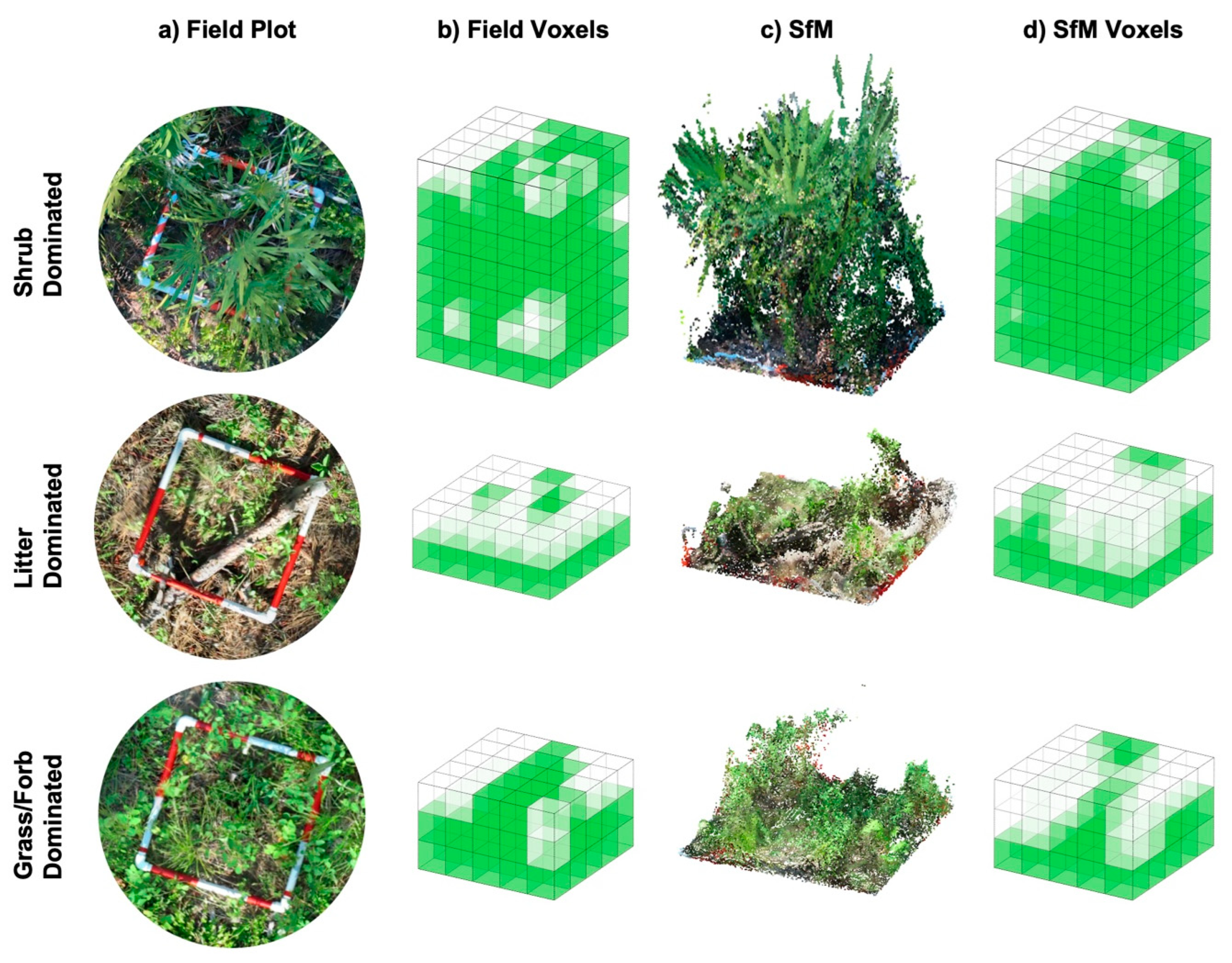
Photogrammetric models were generated for all 145 plots, but 7 plots were removed from subsequent analyses for a total of 138 plots available for analysis. Georeferencing data were not collected for five plots at THB, and therefore these were not used in the analysis, and two plots (one at THA and one at LUB) contained vegetation in the uppermost strata that failed to register in the point cloud, leading to large, unexpected discrepancies between sampled biomass, field-sampled metrics, and SfM metrics. Visual inspection of the remaining raw point clouds generally showed strong representation of vegetation structure, height, and color, although many models often contained small artifacts of spurious mid-air points, resulting in misestimation of the point cloud height and occupied volume (Figure 3). In most plots, there were strong relationships between field measures and SfM measures of occupied volume and height.
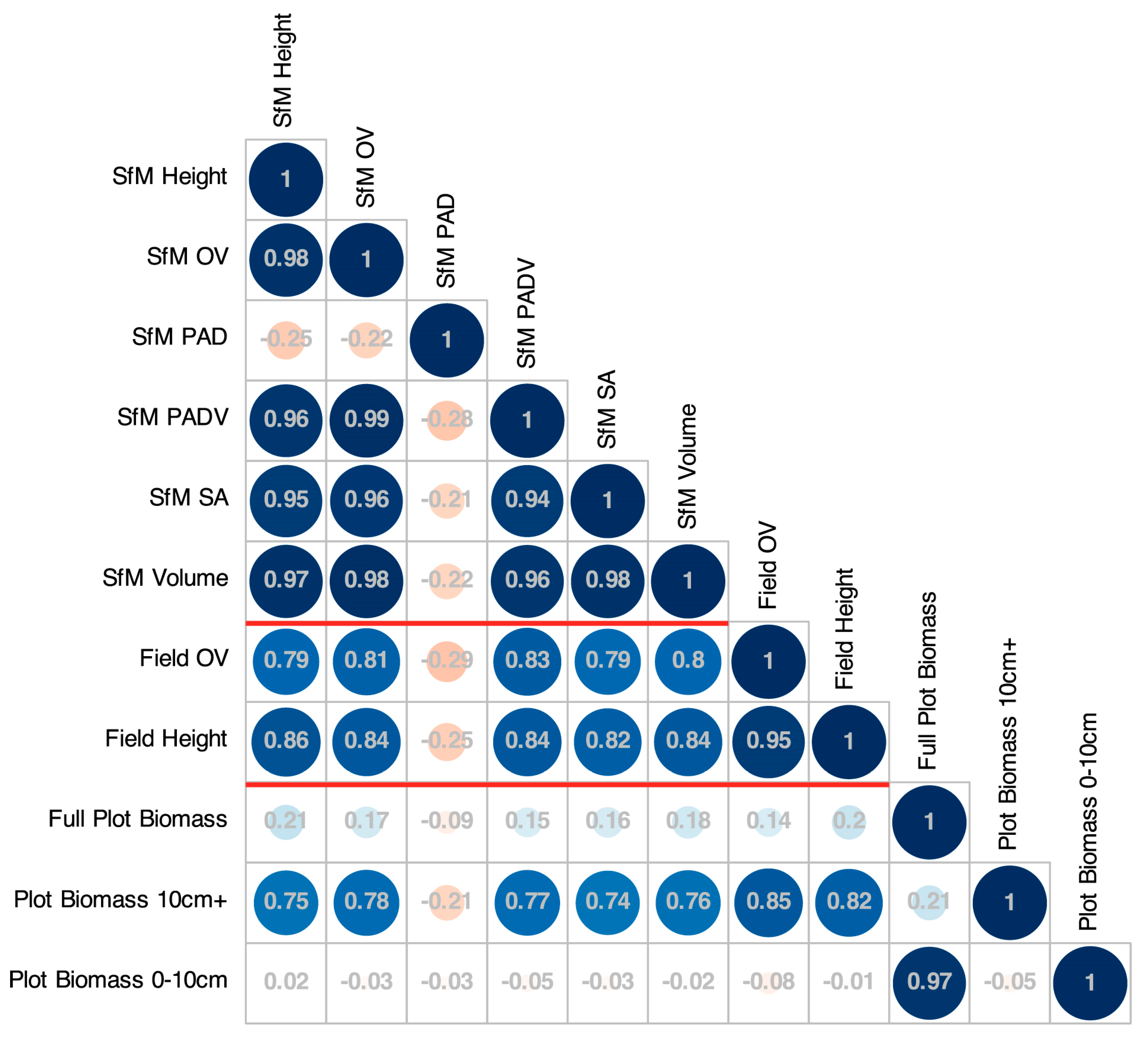
Across all point cloud representations of sample plots, SfM-based metrics were generally strongly and positively correlated (Figure 4). The one exception was SfM PAD, which was weakly and negatively correlated with other metrics. Among the five correlated metrics (SfM Height, SfM OV, SfM PADV, SfM SA, and SfM Volume), correlations ranged from 0.94 (SfM PADV and SfM SA) to 0.99 (SfM PADV and SfM OV). Because of this, we focused on univariate linear regression models to predict biomass to avoid issues with multicollinearity.
In plots with dense vegetation, such as shrub-dominated plots at the Tate’s Hell sites, occlusion from the upper strata of vegetation resulted in incomplete representations of interior vegetation and the lowest fuel stratum. By contrast, within timber litter-dominated plots such as those at Lubrecht, the lowest stratum of fuel was often only represented as a thin, homogenous layer of points. Occlusion in the lowest stratum was evident in preliminary evaluation of photogrammetry metrics and biomass; while our metrics were poorly correlated with total plot biomass (R = −0.08 to 0.21), they were strongly correlated with the remaining biomass when the lowest stratum of vegetation was removed (R = 0.74 to 0.85, excluding SfM PAD). Due to issues of occlusion and weak correlations with biomass in the 0–10 cm stratum, we focused on biomass models above 10 cm (Plot Biomass 10 cm+, Figure 4) and did not evaluate a litter-only fuel model. The lowest stratum was included in our comparisons between field-derived and SfM-derived height and occupied volume.

3.2. Comparison of Point Cloud Metrics to Field Data

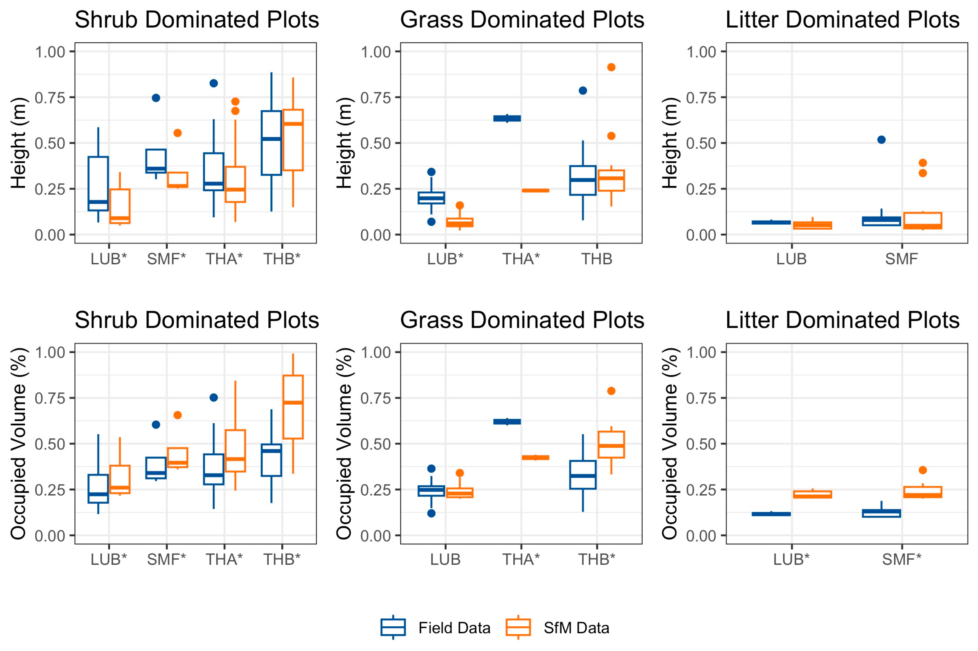
SfM Height was positively correlated with Field Height (R = 0.86 across all plots), but point clouds tended to underestimate average height compared to the field sampling data (Figure 5). These differences were most pronounced in our grass-dominated plots at Lubrecht and Tate’s Hell A, where in-field sampling may have captured tall blades of grass that could not be resolved in the point cloud models. In grass-dominated plots at Lubrecht, the median fuel height was 20 cm based on field sampling data and 6 cm in point cloud representations. At Tate’s Hell A, the median height from field sampling in grass-dominated plots was 63 cm, but only 24 cm according to the photogrammetry models. In shrub-dominated plots, SfM Height was generally lower than Field Height, but differences were less pronounced than in the grass-dominated sites. The closest agreement between SfM Height and Field Height occurred in the litter-dominated plots, but heights were generally very low (under 10 cm for most plots).
While the photogrammetry models tended to have lower fuel heights than field estimations, they generally overestimated field-measured occupied volume (Figure 5). For all fuel types across all sites, the median SfM OV was higher than the median Field OV, except for grass-dominated plots at Lubrecht and Tate’s Hell A. The most pronounced differences between Field and SfM OV were in the shrub-dominated plots at Tate’s Hell A and Tate’s Hell B.

3.3. Modeling Biomass with Photogrammetry Metrics

3.3.1. Grass-Dominated Plots

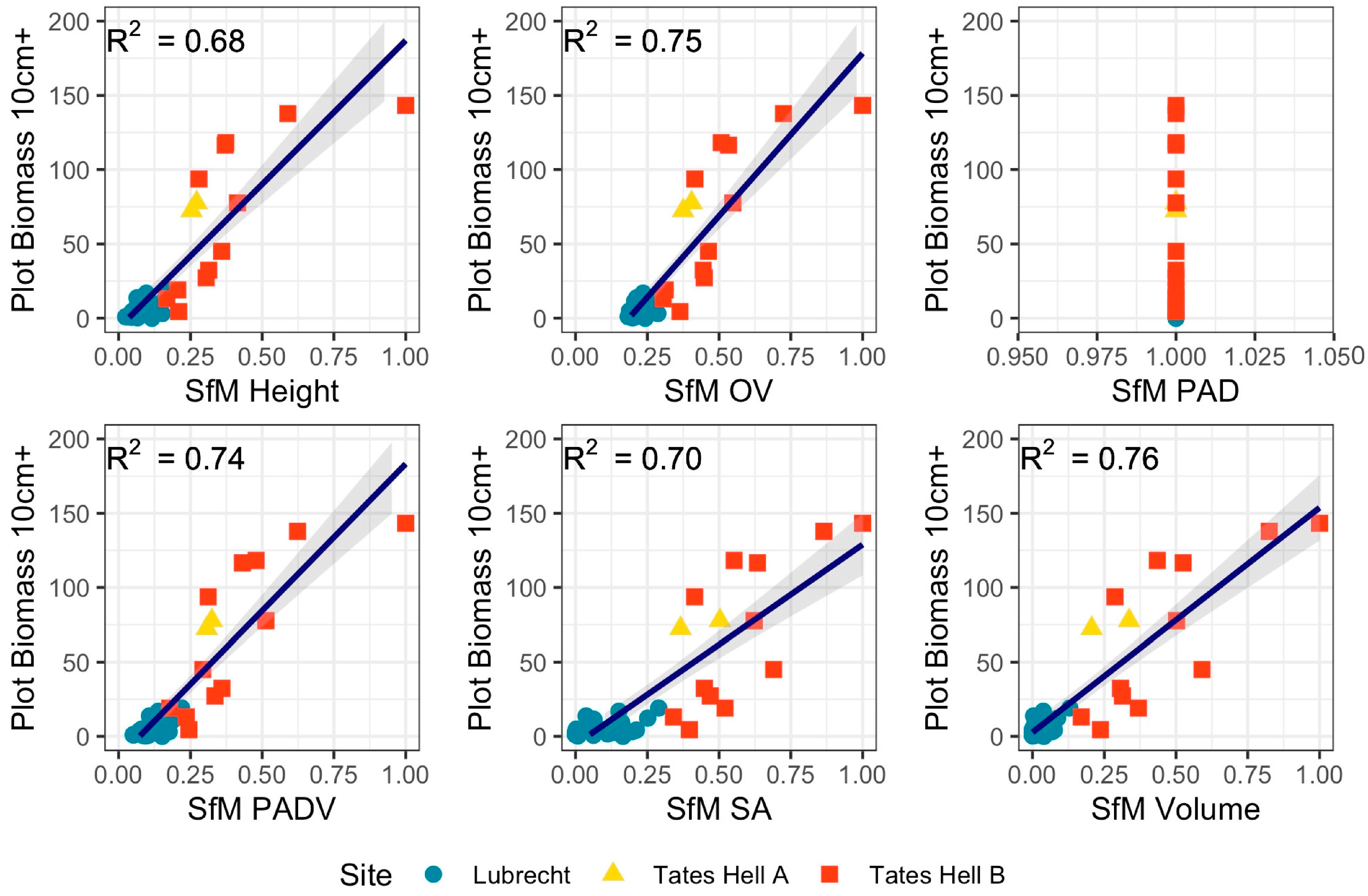
With the exception of PAD, SfM-based metrics had strong relationships with plot biomass above 10 cm in the 42 grass-dominated plots across Lubrecht, Tate’s Hell A, and Tate’s Hell B (Table 2, Figure 6). There were no grass-dominated plots at Sycan Forest. The best performing model was SfM Volume, which was positively correlated with biomass and had a high coefficient of determination (R2 = 0.76, rRMSE = 74%). Biomass above 10 cm in these plots ranged between 0 g in a sparsely vegetated plot at Lubrecht and 143.25 g at a plot with saw palmetto present in the upper strata at Tate’s Hell B (Table 3).

3.3.2. Shrub-Dominated Plots

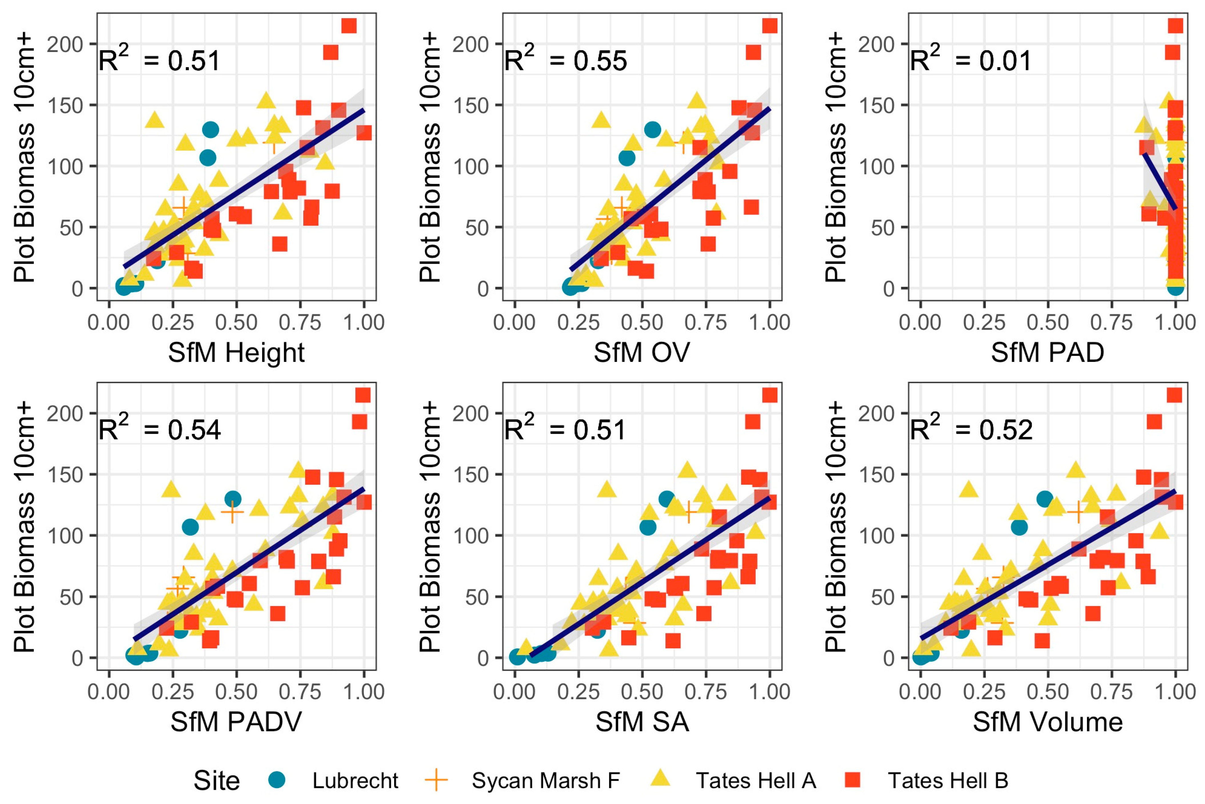
Among the plots included in our analysis, the majority of plots were dominated by shrubs (n = 79), with the highest representation in the southeastern Tate’s Hell sites. As a field sampling category, “shrubs” included hardwood deciduous shrubs, evergreen shrubs, and shrub-like palms including saw palmetto, and therefore represented a broad range of shrub types and associated biomass. Plot biomass above 10 cm in shrub-dominated plots ranged from 0.67 g at Lubrecht to 214.82 g at Tate’s Hell B (Table 3). The SfM OV model had the strongest relationship with biomass (adjusted R2 = 0.55, rRMSE = 46%), closely followed by SfM PADV (adjusted R2 = 0.54, rRMSE = 46%) (Figure 7, Table 2).

3.3.3. Global Model

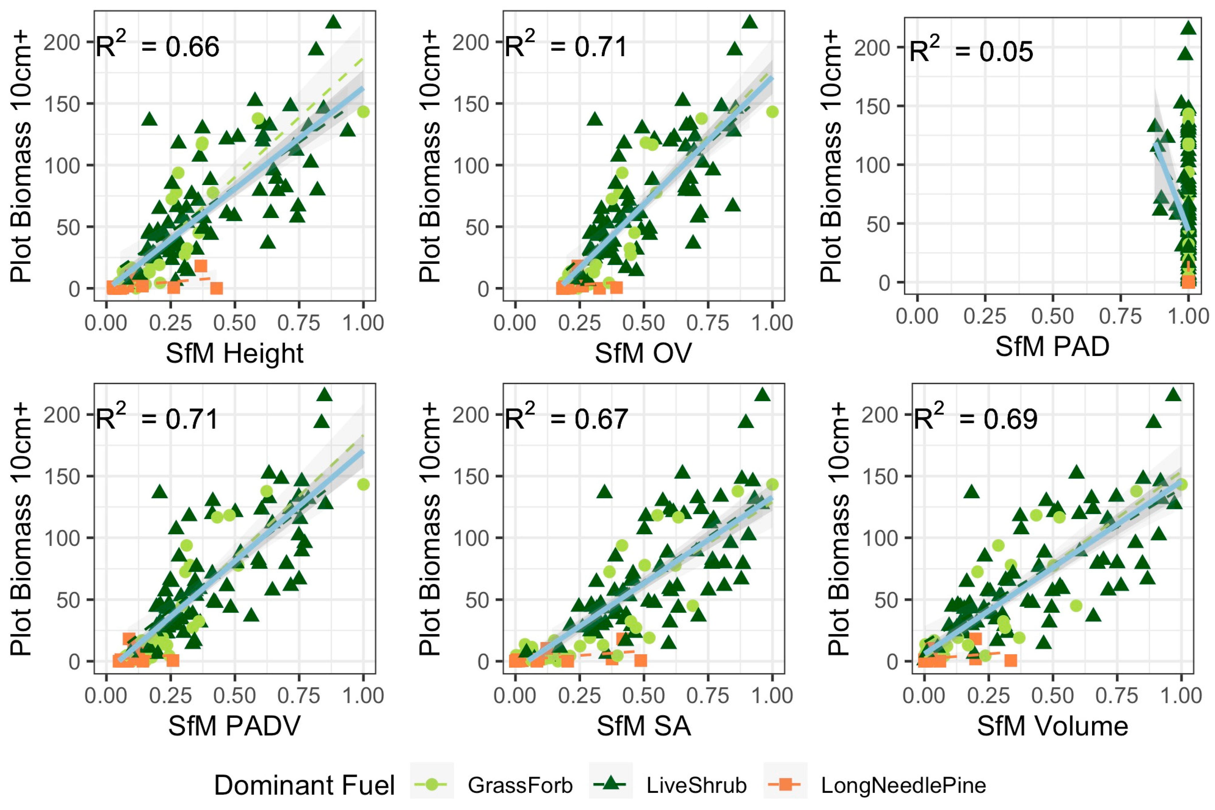
In global models (Figure 8), which included all plots regardless of fuel type, SfM OV and SfM PADV had the strongest relationships with biomass above 10 cm (R2 = 0.71, rRMSE = 56% for both models), but SfM OV had a slightly lower Akaike Information Criterion (AIC) value (1292.69 vs. 1292.93, Table S1 in Supplementary). SfM Volume, SfM SA, and SfM Height models were comparable in model performance. By contrast, SfM PAD had no correlation with biomass. Biomass in our global models ranged from 0 g above 10 cm in grass- and litter-dominated sites at Lubrecht to 214.82 g above 10 cm in shrub-dominated plots at Tate’s Hell B (Table 3).

3.3.4. Global Model with Fuel Type

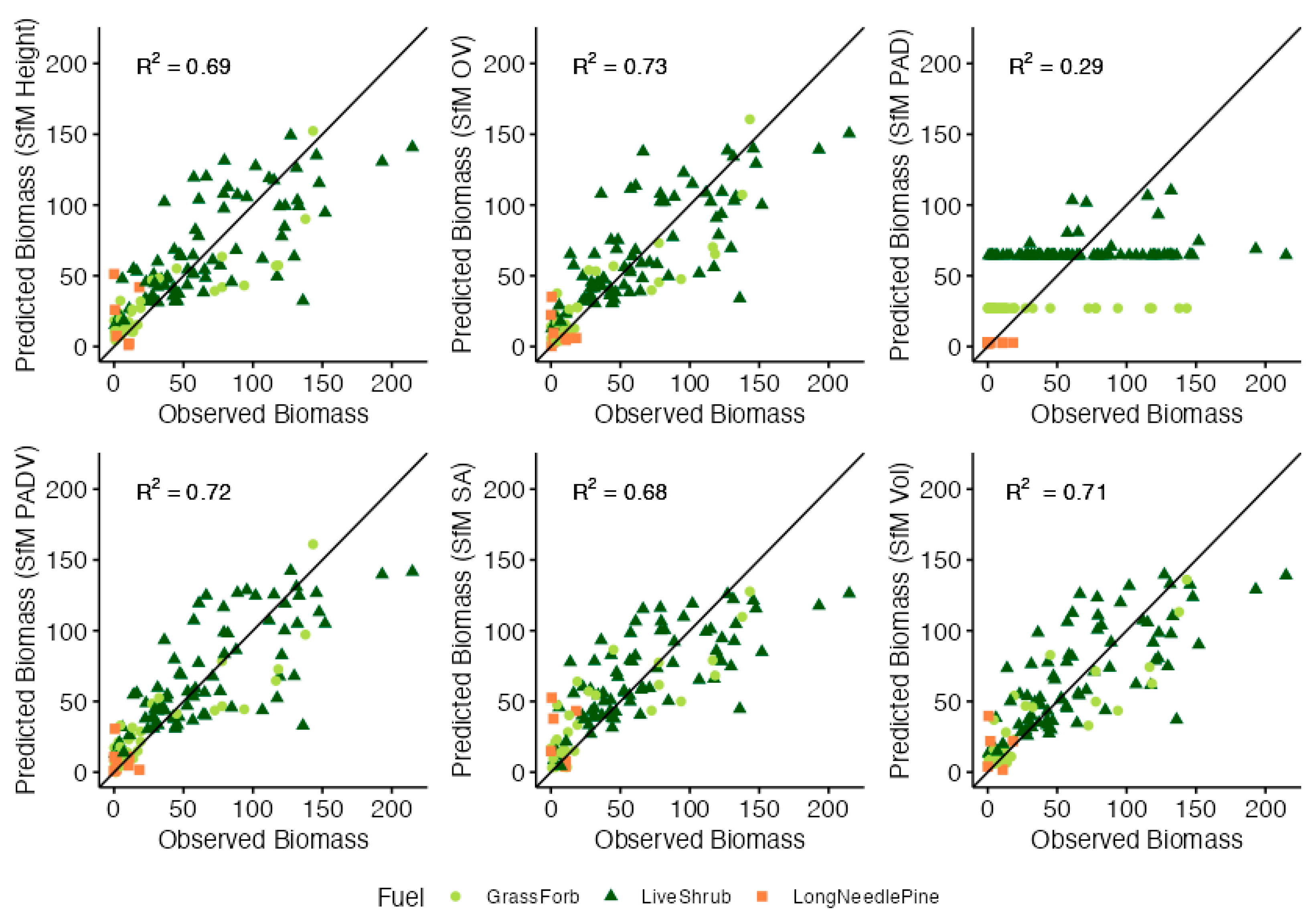
Global models that incorporated fuel type as a categorical variable were marginally improved in the ANCOVA model (Figure 9). The best-performing models were those that incorporated SfM OV and SfM PADV—both models had similar variance explained (R2 = 0.73 for OV and 0.72 for PADV), though the OV model had a slightly better AIC value (1292.14 vs. 1294.42, Table S2 in Supplementary Materials).

4. Discussion

We evaluated the ability of close-range structure-from-motion (SfM) point clouds to characterize the 3D understory fuel structure and predict understory biomass in 138 plots across four forested sites, representing two southeastern pine flatwood sites and two western ponderosa pine sites. Our study focused on three primary research questions: (1) how well do photogrammetric point clouds characterize fuel structure compared to field sampling? (2) Can measures of fuel structure from photogrammetric point clouds be used to develop predictive models of biomass? (3) How generalizable are these models across different fuel complexes and forest types? To our knowledge, this study represents the largest sample of image-based point clouds analyzed for understory fuel characterization, and the only study to evaluate predictive ability across different forest types. We present a novel, video-based approach for rapid data collection that demonstrates potential across multiple domains and present a suite of metrics that can be used to summarize point cloud models.
Videos collected from a handheld GoPro camera produced SfM point clouds with reliable representations of fuel height and structure across our sites (Figure 3). While previous studies that have assessed the applications of close-range SfM have largely relied on individually collected photographs to create point clouds [21,22,23,24], the method presented here offers an efficient, affordable way to collect data with a single video taken in just under two minutes per plot. In this study, we relied on a combination of Python scripts and processing workflows in the commercial software Agisoft Metashape to produce point clouds for each sampling plot; this constituted a semi-automated approach that required manual input to define point cloud reference points and spatial scale. We recognize that accessibility and a simple user pipeline will be critical for wider adoption of this method. For example, migrating to a cloud-hosted open source SfM code library would allow for the automated processing of videos to point clouds and ingestion-to-analysis workflows that provide a large library of outputs that can then be embedded into deep learning networks to improve coarser-scale fuel mapping.

4.1. How Well Do Photogrammetric Point Clouds Characterize Fuel Structure Compared to Field Sampling?

The SfM models had strong agreement with field data for estimates of average fuel height (R = 0.86 across all plots), though SfM models typically underestimated height compared to field sampling. This finding is similar to previous studies, which found that field-estimated heights tended to be greater than those estimated from photogrammetry [21]. Although our SfM processing included a workflow to define spatial scales in the x and y directions, we did not explicitly define spatial scales in the z. This may have resulted in minor distortions of point cloud height across the models. Differences in height between the SfM and field data were likely compounded by the inherent limitations to voxel-based field sampling, which may in contrast overestimate heights if small amounts of vegetation are present in the lowest portion of a single voxel (Figure 5). For example, if a voxel in the 30 to 40 cm height stratum contained grasses only 31 cm high, the full voxel would have been cataloged as occupied in the field data, resulting in a height measurement of 40 cm.
Occupied volume (OV) based on SfM also had strong relationships with field-measured OV (R = 0.81 across all plots), but SfM tended to overestimate OV compared to field sampling (see Figure 3). This result contrasted with a previous study that found field-sampling to overestimate volume compared to remote sensing methods [8]. However, unlike laser-based remote sensing methods such as terrestrial lidar scanning, which produce highly accurate estimates of depth and distance by measuring light pulse returns, SfM relies solely on what the camera views, which is dependent on sampling angle, shadowing, and potential occlusion from proximal objects. While this may have resulted in occlusion of interior vegetation in densely vegetated plots, it frequently resulted in random noise and spurious mid-air points that contributed to the overestimation of occupied volume as voxels were falsely calculated as occupied. This effect was most pronounced in the shrub (saw palmetto)-dominated plots of THB, where dense configurations of tall fuels resulted in slightly less-resolved and noisier point clouds. The exception to this overestimation was in grass-dominated plots at THA (n = 2); in these plots, grasses were relatively tall compared to other sites and did not register in the SfM models. At grass-dominated plots in LUB and THB, grasses tended to be lower and more uniform in their configurations.

4.2. Can Measures of Fuel Structure from Photogrammetric Point Clouds Be Used to Develop Predictive Models of Biomass?

We found that nearly all structural metrics calculated from the SfM point clouds were strongly correlated and performed similarly well in predictive models of biomass above 10 cm height. Conceptually, these metrics are quite similar and rely on similar calculations. For example, SfM Height relies on the same voxelization process as SfM OV, and SfM Volume is the interior volume calculated from the outer hull used to determine SfM SA. The close relationships of these metrics are therefore expected. The SfM PAD metric offers an exception and was not highly correlated with other metrics, but was highly skewed in its distribution and could not be used reliably as a covariate in our models. Our SfM PAD calculation was developed based on the theory that ground-normalized point clouds of horizontally discontinuous fuel beds would produce variable values to reflect mosaics of fuel and bare ground when evaluated in the x and y directions. However, nearly all the plots in our analysis had the same maximum SfM PAD value of 100% percent occupied. While this may legitimately reflect that some plots were indeed horizontally continuous with fuel, it also reflects the relatively poor characterization of the lowest fuel stratum, as near-ground fuel and actual ground points were often indistinguishable from one another in the 3D models.
Despite the close collinearity between most of our metrics, SfM OV and our novel SfM PADV metric were consistently the best metrics for predicting biomass above 10 cm in all fuel types. Point cloud volume from TLS has been used to predict biomass in previous studies with moderate to high accuracy [8,20,38,39]. Vertical plant area profiles and vertical leaf area density from voxelized point clouds have similarly been used to characterize 3D structure for biomass modeling, but estimations of these metrics have typically been derived from more complex equations calculated at finer scales that take lidar measurement angles into account [33,40,41]. Our SfM PADV calculation as a measure of vertical fuel profile is relatively simplistic—no knowledge or extraction of camera angles is required—while inherently accounting for the other metrics that were found to be similarly strong predictors of biomass in this study (i.e., height and occupied volume). At a 1 cm3 voxel resolution, our calculation captured fuel structure variability without compromising computational speed.
Remotely sensed structural metrics such as height and volume have been used as reliable predictors of biomass in shrubs [20,36,39,42], and to a lesser extent in grasses and forbs [38,43]. By contrast, we found that grass-only models overall performed better than shrub-only models in our study. This is likely an effect of how we attributed fuel types to our plots across different sites. Plots attributed as grass-dominated according to occupied voxel counts were often co-dominated by shrubs, especially in THA and THB, where saw palmetto, gallberry, and Vaccinium spp. were often present in near-equal amounts to grasses. Shrub-dominated plots also often contained grasses or forbs, but in lesser amounts. Because of this, the performance of our grass models may in reality better reflect the ability of SfM metrics to predict biomass in mixed shrub–grass complexes rather than pure grass alone.

4.3. How Generalizable Are These Models across Different Fuel Complexes and Forest Types?

Our results suggest that SfM metrics are best able to predict biomass when models account for complexes of fuels rather than individual, discrete fuel types. This is reflected in our global model, which implicitly accounted for mixed fuel beds, and performed better than shrub-only models and nearly as well as grass-only models (Table 2). Our method of assigning fuel type dominance using occupied volume field surveys was admittedly simplistic and could not account for co-dominant fuels, which were fairly common in our dataset (see Figure 3). Pure fuel types are relatively rare in wildland fuel characterization [44], and future work should focus on developing more nuanced classification systems that categorize plots as complexes of fuels rather than single fuel types. Although our sample size (n = 138) was relatively large compared to previous studies, it was still insufficient to evaluate a range of fuel type classifications for mixed-fuel complexes.
While our models demonstrated promising relationships between plot-level summary metrics and biomass above 10 cm height in shrub and grass complexes, relationships with the lowest fuel strata were more variable. Across all sites, SfM metrics were poorly correlated with biomass that included the lowest litter layer of vegetation. Unlike laser-based remote sensing techniques that can penetrate the litter layer to capture variation in depth and porosity, SfM-based models of litter essentially represent the outer hull of fuels. Our global ANCOVA models that explicitly accounted for fuel type in each plot produced only a marginally better fit than our global models which did not account for fuel type at all, suggesting that further method refinements to accurately characterize litter-dominated plots are required before this technique can be fully generalizable across different complexes of fuels. While these results justify the need for a more sensitive method to accurately characterize the lowest fuel strata, biomass above the litter layer represents the bulk of vegetation relevant to planning fuel treatments and understanding patterns of fire behavior and spread [45,46]. This method also offers a promising approach for characterizing and mapping understory vegetation for the assessment of wildlife habitat [2,47] and above-ground carbon storage [39,43,48]. In future work, spatially explicit models that characterize all fuel layers and minimize the occlusion of interior and ground-level fuels may expand the utility of this method for use in evaluations of post-fire fuel consumption [30] and next-generation fire behavior models. Within multilayered fuel beds, accurate characterizations of the forest floor using remote sensing methods will remain a challenge.

5. Conclusions

Close-range photogrammetry has demonstrated promise as an alternative to traditional fuel sampling and more costly remote sensing techniques [21,22,23,24,38]. However, no previous study that we are aware of has incorporated such a large dataset (n = 138 plots across four sites and two forest types) to evaluate the potential of a video-based technique for robust structure characterization and biomass estimation. This work advances our understanding of the utility of close-range photogrammetry in two regards: (1) we show that handheld video cameras can be used to decrease the time and effort involved in photogrammetric image collection, and (2) the performance of this technique was evaluated across different fuel complexes and forest types. Our technique performed best in shrub-dominated and grass/forb-dominated plots across all sites; our technique performed most poorly in litter-dominated plots, as the photogrammetry point clouds were unable to adequately characterize the 0–10 cm fuel stratum due to occlusion. In the short term, our technique offers land managers an affordable potential alternative to time-consuming field sampling; in the long term, this method may be used as an efficient way to bolster machine learning training datasets for broader-scale predictive models of fuel type and biomass.
Additionally, we recognize that the analyses conducted in this study inherently rely on manual attribution of fuel types to group plots into relevant models. To be fully useful for managers as an alternative to field sampling, this fuel typing would need to be accomplished through automated processes with minimal user input. Future applications of this technique could incorporate the color information (red-green-blue (RGB) values) of each SfM point cloud to automatically attribute each plot with a fuel type based on combinations of color information and structural characteristics informed by machine learning. Previous studies that have fused spectral and structural characteristics for fuel classification have had variable success in characterizing fuels below the canopy [49,50,51]; more work is needed to inform accurate understory fuel characterization. More robust structural metrics like those presented here, combined with visible-band spectral indices, could implicitly account for different fuel complexes and result in broader applications of this method to improve the accessibility of 3D understory fuel structure and biomass characterization [7,52].

Supplementary Materials

The following supporting information can be downloaded at: https://www.mdpi.com/article/10.3390/rs15194837/s1, Figure S1: Workflow diagram to produce point clouds from GoPro video; Figure S2: Observed versus predicted values of biomass above 10 cm for grass models; Figure S3: Observed versus predicted values of biomass above 10 cm for shrub models; Figure S4: Observed versus predicted values of biomass above 10 cm for global models; Table S1: Akaike Information Criterion (AIC) for global models; Table S2: Akaike Information Criterion (AIC) for global models accounting for fuel type.

Author Contributions

Conceptualization, G.R.C., S.J.P. and E.R.; Data curation, G.R.C., S.J.P., B.D., P.E. and D.G.N.; Formal analysis, G.R.C. and S.J.P.; Investigation, S.J.P., E.R. and D.G.N., Methodology, G.R.C., S.J.P. and E.R.; Resources, S.J.P. and E.R.; Software, G.R.C. and B.D.; Visualization, G.R.C. and B.D.; Writing—original draft, G.R.C.; Writing—review and editing, G.R.C., S.J.P., E.R., B.D., P.E., M.C.K. and D.G.N. All authors have read and agreed to the published version of the manuscript.

Funding

This work was supported by funding from the US Department of Defense Strategic and Environmental Research and Development Program, project number RC19-C1-1064.

Data Availability Statement

Relevant scripts and datasets are available on our Open Science Framework site: https://osf.io/4sdgb/.

Conflicts of Interest

The authors declare no conflict of interest.

References

  1. Li, S.; Wang, T.; Hou, Z.; Gong, Y.; Feng, L.; Ge, J. Harnessing terrestrial laser scanning to predict understory biomass in temperate mixed forests. Ecol. Indic. 2021, 121, 107011. [Google Scholar] [CrossRef]
  2. Martinuzzi, S.; Vierling, L.A.; Gould, W.A.; Falkowski, M.J.; Evans, J.S.; Hudak, A.T.; Vierling, K.T. Mapping snags and understory shrubs for a LiDAR-based assessment of wildlife habitat suitability. Remote Sens. Environ. 2009, 113, 2533–2546. [Google Scholar] [CrossRef]
  3. Moore, P.T.; Van Miegroet, H.; Nicholas, N.S. Relative role of understory and overstory in carbon and nitrogen cycling in a southern Appalachian spruce–fir forest AES Publication 7863. Utah Agricultural Experiment Station, Utah State University, Logan, Utah. Can. J. For. Res. 2007, 37, 2689–2700. [Google Scholar] [CrossRef]
  4. Muir, P.S.; Mattingly, R.L.; Tappeiner, J.C., II; Bailey, J.D.; Elliott, W.E.; Hagar, J.C.; Miller, J.C.; Peterson, E.B.; Starkey, E.E. Managing for Biodiversity in Young Douglas-Fir Forests of Western Oregon (Biological Science Report); U.S. Geological Survey: Reston, VA, USA; Forest and Rangeland Ecosystem Science Center: Corvallis, OR, USA, 2002. [Google Scholar]
  5. Kerns, B.K.; Ohmann, J.L. Evaluation and prediction of shrub cover in coastal Oregon forests (USA). Ecol. Indic. 2004, 4, 83–98. [Google Scholar] [CrossRef]
  6. Powell, T.L.; Gholz, H.L.; Clark, K.L.; Starr, G.; Cropper, W.P., Jr.; Martin, T.A. Carbon exchange of a mature, naturally regenerated pine forest in north Florida. Glob. Change Biol. 2008, 14, 2523–2538. [Google Scholar] [CrossRef]
  7. Hiers, J.K.; O’Brien, J.J.; Mitchell, R.J.; Grego, J.M.; Loudermilk, E.L. The wildland fuel cell concept: An approach to characterize fine-scale variation in fuels and fire in frequently burned longleaf pine forests. Int. J. Wildland Fire 2009, 18, 315–325. [Google Scholar] [CrossRef]
  8. Loudermilk, E.L.; Hiers, J.K.; O’Brien, J.J.; Mitchell, R.J.; Singhania, A.; Fernandez, J.C.; Cropper, W.P.; Slatton, K.C. Ground-based LIDAR: A novel approach to quantify fine-scale fuelbed characteristics. Int. J. Wildland Fire 2009, 18, 676–685. [Google Scholar] [CrossRef]
  9. Loudermilk, E.L.; O’Brien, J.J.; Mitchell, R.J.; Cropper, W.P.; Hiers, J.K.; Grunwald, S.; Grego, J.; Fernandez-Diaz, J.C. Linking complex forest fuel structure and fire behaviour at fine scales. Int. J. Wildland Fire 2012, 21, 882. [Google Scholar] [CrossRef]
  10. Agee, J. Fire Ecology of Pacific Northwest Forests; Island Press: Washington, DC, USA, 1993. [Google Scholar]
  11. Mitchell, R.J.; Hiers, J.K.; O’Brien, J.; Starr, G. Ecological forestry in the Southeast: Understanding the ecology of fuels. J. For. 2009, 107, 391–397. [Google Scholar]
  12. Keane, R.E. Describing wildland surface fuel loading for fire management: A review of approaches, methods and systems. Int. J. Wildland Fire 2009, 22, 51–62. [Google Scholar] [CrossRef]
  13. Wright, C.; Vilnakek, R.; Ottmar, R.; Eagle, P. Digital Photo Series (Natural Fuels Photo Series). JFSP Res. Proj. Rep. 2007; 116. [Google Scholar]
  14. Brown, J.K.; Oberheu, R.D.; Johnston, C.M. Handbook for Inventorying Surface Fuels and Biomass in the Interior West (No. INT-GTR-129); U.S. Department of Agriculture: Washington, DC, USA; Forest Service: Washington, DC, USA; Intermountain Forest and Range Experiment Station: Ogden, UT, USA, 1982. [Google Scholar] [CrossRef]
  15. Bright, B.C.; Hudak, A.T.; Meddens, A.J.H.; Hawbaker, T.J.; Briggs, J.S.; Kennedy, R.E. Prediction of Forest Canopy and Surface Fuels from Lidar and Satellite Time Series Data in a Bark Beetle-Affected Forest. Forests 2017, 8, 322. [Google Scholar] [CrossRef]
  16. White, J.C.; Coops, N.C.; Wulder, M.A.; Vastaranta, M.; Hilker, T.; Tompalski, P. Remote Sensing Technologies for Enhancing Forest Inventories: A Review. Can. J. Remote Sens. 2016, 42, 619–641. [Google Scholar] [CrossRef]
  17. Calders, K.; Adams, J.; Armston, J.; Bartholomeus, H.; Bauwens, S.; Bentley, L.P.; Chave, J.; Danson, F.M.; Demol, M.; Disney, M.; et al. Terrestrial laser scanning in forest ecology: Expanding the horizon. Remote Sens. Environ. 2020, 251, 112102. [Google Scholar] [CrossRef]
  18. Dassot, M.; Constant, T.; Fournier, M. The use of terrestrial LiDAR technology in forest science: Application Fields, Benefits and Challenges. Ann. For. Sci. 2011, 68, 959–974. [Google Scholar] [CrossRef]
  19. Liang, X.; Kankare, V.; Hyyppä, J.; Wang, Y.; Kukko, A.; Haggrén, H.; Yu, X.; Kaartinen, H.; Jaakkola, A.; Guan, F.; et al. Terrestrial laser scanning in forest inventories. ISPRS J. Photogramm. Remote Sens. 2016, 115, 63–77. [Google Scholar] [CrossRef]
  20. Rowell, E.; Loudermilk, E.L.; Hawley, C.; Pokswinski, S.; Seielstad, C.; Queen, L.L.; O’Brien, J.J.; Hudak, A.T.; Goodrick, S.; Hiers, J.K. Coupling terrestrial laser scanning with 3D fuel biomass sampling for advancing wildland fuels characterization. For. Ecol. Manag. 2020, 462, 117945. [Google Scholar] [CrossRef]
  21. Bright, B.C.; Loudermilk, E.L.; Pokswinski, S.M.; Hudak, A.T.; O’Brien, J.J. Introducing Close-Range Photogrammetry for Characterizing Forest Understory Plant Diversity and Surface Fuel Structure at Fine Scales. Can. J. Remote Sens. 2016, 42, 460–472. [Google Scholar] [CrossRef]
  22. Piermattei, L.; Karel, W.; Wang, D.; Wieser, M.; Mokroš, M.; Surový, P.; Koreň, M.; Tomaštík, J.; Pfeifer, N.; Hollaus, M. Terrestrial Structure from Motion Photogrammetry for Deriving Forest Inventory Data. Remote Sens. 2019, 11, 950. [Google Scholar] [CrossRef]
  23. Wallace, L.; Hillman, S.; Reinke, K.; Hally, B. Non-destructive estimation of above-ground surface and near-surface biomass using 3D terrestrial remote sensing techniques. Methods Ecol. Evol. 2017, 8, 1607–1616. [Google Scholar] [CrossRef]
  24. Wallace, L.; Hally, B.; Hillman, S.; Jones, S.D.; Reinke, K. Terrestrial Image-Based Point Clouds for Mapping Near-Ground Vegetation Structure: Potential and Limitations. Fire 2020, 3, 59. [Google Scholar] [CrossRef]
  25. Churchill, D.; Jeronimo, S.; Larson, A.; Fischer, P.; Dahlgreen, M.; Franklin, J. The ICO Approach to Quantifying and Restoring Forest Spatial Pattern: Implementation Guide. ICO App. 2016, 3. [Google Scholar]
  26. Roussel, J.; Auty, D.; Coops, N.C.; Tompalski, P.; Goodbody, T.R.; Meador, A.S.; Bourdon, J.; de Boissieu, F.; Achim, A. lidR: An R package for analysis of Airborne Laser Scanning (ALS) data. Remote Sens. of Environ. 2020, 251, 112061. [Google Scholar] [CrossRef]
  27. Roussel, J.; Auty, D. Airborne LiDAR Data Manipulation and Visualization for Forestry Applications. R package version 4.0.1. 2022. Available online: https://cran.r-project.org/package=lidR (accessed on 20 May 2022).
  28. Hawley, C.M.; Loudermilk, E.L.; Rowell, E.M.; Pokswinski, S. A novel approach to fuel biomass sampling for 3D fuel characterization. MethodsX 2018, 5, 1597–1604. [Google Scholar] [CrossRef] [PubMed]
  29. R Core Team. R: A Language and Environment for Statistical Computer; R Foundation for Statistical Computing: Vienna, Austria, 2021; Available online: http://www.R-project.org/ (accessed on 1 February 2021).
  30. Hudak, A.T.; Kato, A.; Bright, B.C.; Loudermilk, E.L.; Hawley, C.; Restaino, J.C.; Ottmar, R.D.; Prata, G.A.; Cabo, C.; Prichard, S.J.; et al. Towards Spatially Explicit Quantification of Pre- and Postfire Fuels and Fuel Consumption from Traditional and Point Cloud Measurements. For. Sci. 2020, 66, 428–442. [Google Scholar] [CrossRef]
  31. Brown, S. Measuring carbon in forests: Current status and future challenges. Environ. Pollut. 2002, 116, 363–372. [Google Scholar] [CrossRef] [PubMed]
  32. Chave, J.; Andalo, C.; Brown, S.; Cairns, M.A.; Chambers, J.Q.; Eamus, D.; Fölster, H.; Fromard, F.; Higuchi, N.; Kira, T.; et al. Tree allometry and improved estimation of carbon stocks and balance in tropical forests. Oecologia 2005, 145, 87–99. [Google Scholar] [CrossRef]
  33. Hosoi, F.; Omasa, K. Estimation of vertical plant area density profiles in a rice canopy at different growth stages by high-resolution portable scanning lidar with a lightweight mirror. ISPRS J. Photogramm. Remote Sens. 2012, 74, 11–19. [Google Scholar] [CrossRef]
  34. Lecigne, B. VoxR: Trees Geometry and Morphology from Unstructure TLS Data. R package version 1.0.0. 2020. Available online: https://cran.r-project.org/package=VoxR (accessed on 21 February 2021).
  35. Roussel, J.; Barber, C.B.; Habel, K.; Grasman, R.; Gramacy, R.B.; Mozharovskyi, S.D. Geometry: Mesh Generation and Surface Tessellation. R package version 0.4.6.1. 2022. Available online: http://cran.r-project.org/package=geometry (accessed on 21 February 2021).
  36. Olsoy, P.J.; Glenn, N.F.; Clark, P.E.; Derryberry, D.R. Aboveground total and green biomass of dryland shrub derived from terrestrial laser scanning. ISPRS J. Photogramm. Remote Sens. 2014, 88, 166–173. [Google Scholar] [CrossRef]
  37. Akaike, H. A new look at the statistical model identification. IEEE Trans. Autom. Control 1974, 9, 716–723. [Google Scholar] [CrossRef]
  38. Cooper, S.D.; Roy, D.P.; Schaaf, C.B.; Paynter, I. Examination of the Potential of Terrestrial Laser Scanning and Structure-from-Motion Photogrammetry for Rapid Nondestructive Field Measurement of Grass Biomass. Remote Sens. 2017, 9, 531. [Google Scholar] [CrossRef]
  39. Greaves, H.E.; Vierling, L.A.; Eitel, J.U.H.; Boelman, N.T.; Magney, T.S.; Prager, C.M.; Griffin, K.L. Estimating aboveground biomass and leaf area of low-stature Arctic shrubs with terrestrial LiDAR. Remote Sens. Environ. 2015, 164, 26–35. [Google Scholar] [CrossRef]
  40. Hosoi, F.; Omasa, K. Voxel-Based 3-D Modeling of Individual Trees for Estimating Leaf Area Density Using High-Resolution Portable Scanning Lidar. IEEE Trans. Geosci. Remote Sens. 2006, 44, 3610–3618. [Google Scholar] [CrossRef]
  41. Hosoi, F.; Omasa, K. Estimating vertical plant area density profile and growth parameters of a wheat canopy at different growth stages using three-dimensional portable lidar imaging. ISPRS J. Photogramm. Remote Sens. 2009, 64, 151–158. [Google Scholar] [CrossRef]
  42. Poley, L.G.; Laskin, D.N.; McDermid, G.J. Quantifying Aboveground Biomass of Shrubs Using Spectral and Structural Metrics Derived from UAS Imagery. Remote Sens. 2020, 12, 2199. [Google Scholar] [CrossRef]
  43. Anderson, K.E.; Glenn, N.F.; Spaete, L.P.; Shinneman, D.J.; Pilliod, D.S.; Arkle, R.S.; McIlroy, S.K.; Derryberry, D.R. Estimating vegetation biomass and cover across large plots in shrub and grass dominated drylands using terrestrial lidar and machine learning. Ecol. Indic. 2018, 84, 793–802. [Google Scholar] [CrossRef]
  44. Loudermilk, E.L.; Hiers, J.K.; O’Brien, J.J. The role of fuels for understanding fire behavior and fire effects. In Ecological Restoration and Management of Longleaf Pine Forests; CRC Press: Boca Raton, FL, USA; Taylor Francis Group: Abingdon, UK, 2018; pp. 107–122. [Google Scholar]
  45. Scott, J.H.; Burgan, R.E. Standard Fire Behavior Fuel Models: A Comprehensive Set for Use with Rothermel’s Surface Fire Spread Model; U.S. Department of Agriculture: Washington, DC, USA; Forest Service: Washington, DC, USA; Rocky Mountain Research Station: Fort Collins, CO, USA, 2005; p. 72. [Google Scholar] [CrossRef]
  46. Ottmar, R.D.; Sandberg, D.V.; Riccardi, C.L.; Prichard, S.J. An overview of the Fuel Characteristic Classification System—Quantifying, classifying, and creating fuelbeds for resource planning. Can. J. For. Res. 2007, 37, 2383–2393. [Google Scholar] [CrossRef]
  47. Olsoy, P.J.; Forbey, J.S.; Rachlow, J.L.; Nobler, J.D.; Glenn, N.F.; Shipley, L.A. Fearscapes: Mapping Functional Properties of Cover for Prey with Terrestrial LiDAR. BioScience 2015, 65, 74–80. [Google Scholar] [CrossRef]
  48. Li, A.; Dhakal, S.; Glenn, N.F.; Spaete, L.P.; Shinneman, D.J.; Pilliod, D.S.; Arkle, R.S.; McIlroy, S.K. Lidar Aboveground Vegetation Biomass Estimates in Shrublands: Prediction, Uncertainties and Application to Coarser Scales. Remote Sens. 2017, 9, 903. [Google Scholar] [CrossRef]
  49. García, M.; Riaño, D.; Chuvieco, E.; Salas, J.; Danson, F.M. Multispectral and LiDAR data fusion for fuel type mapping using Support Vector Machine and decision rules. Remote Sens. Environ. 2011, 115, 1369–1379. [Google Scholar] [CrossRef]
  50. Mutlu, M.; Popescu, S.; Stripling, C.; Spencer, T. Mapping surface fuel models using lidar and multispectral data fusion for fire behavior. Remote Sens. Environ. 2008, 112, 274–285. [Google Scholar] [CrossRef]
  51. Stavros, E.; Coen, J.; Peterson, B.; Singh, H.; Kennedy, K.; Ramirez, C.; Schimel, D. Use of Imaging Spectroscopy and LIDAR to Characterize Fuels for Fire Behavior Prediction. Remote Sens. Appl. Soc. Environ. 2018, 11, 41–50. [Google Scholar] [CrossRef]
  52. Rowell, E.; Loudermilk, E.L.; Seielstad, C.; O’Brien, J. Using simulated 3D surface fuelbeds and terrestrial laser scan data to develop inputs to fire behavior models. Can. J. Remote Sens. 2016, 42, 443–459. [Google Scholar] [CrossRef]
Figure 1. Map of locations and representative photos for four study sites across two forest types used in this study: Sycan Marsh Preserve—Forest (SMF) in OR (ponderosa pine); Lubrecht Experimental Forest (LUB) in MT (ponderosa pine); Tate’s Hell State Forest—Site A (THA) in FL (slash pine); and Tate’s Hell State Forest—Site B (THB) in FL (slash pine).
Remotesensing 15 04837 g001
Figure 2. (a) (top) Example layout of 5 m by 5 m photogrammetry and biomass sampling parent plots (green flags with squares) randomly selected from a grid of parent plots at each site. Each 5 m by 5 m parent plot contained five 0.5 m by 0.5 m voxel sampling plots (plots), arranged with four plots at the northwest, northeast, southwest, and southeast corners, with an additional plot in the center (b).
Remotesensing 15 04837 g002
Figure 3. Visual comparison between field plots (column (a)), results of field occupied voxel surveys (column (b)), photogrammetry point clouds (column (c)), and photogrammetry occupied voxelizations (column (d)) for three dominant fuel types in this study: shrub (first row), litter (second row), and grass/forb (third row). Photogrammetric point clouds often contained spurious mid-air points that influenced estimations of occupied volume, but agreement between SfM voxelization and field-derived occupied voxels was generally high.
Remotesensing 15 04837 g003
Figure 4. Correlation matrix for six photogrammetry (SfM) metrics, two field sampling metrics, and three groupings of plot biomass for all plots included in analysis (n = 138). Larger, darker circles indicate a greater value for Pearson’s correlation coefficient. Light or invisible circles represent weakly correlated metrics (<0.3). Blue corresponds to a positive correlation and red corresponds to a negative correlation.
Remotesensing 15 04837 g004
Figure 5. Distributions of height (top row) and occupied volume (bottom row) between field data (blue) and photogrammetry data (orange) across different fuel types and sites. Asterisks represent statistically significant differences (p < 0.05) between mean field and photogrammetry metric values using paired t-tests.
Remotesensing 15 04837 g005
Figure 6. Linear regression results for 6 separate models using photogrammetry metrics (explanatory variable) as predictors of biomass above 10 cm in height (response variable) in grass/forb-dominated plots. Points represent different sampling plots, where blue circles are plots at Lubrecht Experimental Forest, yellow triangles are plots at Tates Hell A, and red squares are plots at Tates Hell B. There were no grass/forb-dominated plots at Sycan Marsh Forest. The column of values at x = 1.0 in the SfM PAD model (top right plot) is due to a legitimate calculation of SfM PAD = 1.0 for all grass-forb-dominated plots.
Remotesensing 15 04837 g006
Figure 7. Linear regression results for 6 separate models using 6 photogrammetry metrics (explanatory variable) as predictors of biomass above 10 cm in height (response variable) in shrub-dominated plots. Points represent different sampling plots, where blue circles are plots at Lubrecht Experimental Forest, orange crosses are plots at Sycan Marsh Forest, yellow triangles are plots at Tate’s Hell A, and red squares are plots at Tate’s Hell B.
Remotesensing 15 04837 g007
Figure 8. Global model linear regression results for 6 separate models using 6 photogrammetry metrics (explanatory variable) as predictors of biomass above 10 cm in height (response variable). Points represent different sampling plots, where light green circles are grass/forb-dominated plots, dark green triangles are shrub-dominated plots, and orange squares are long needle pine (litter)-dominated plots.
Remotesensing 15 04837 g008
Figure 9. Observed versus predicted values for a global model analysis of covariance (ANCOVA) results for 6 separate models using 6 photogrammetry metrics and categorical fuel type (explanatory variable) as predictors of biomass above 10 cm in height (response variable). Points represent different sampling plots, and are colored by dominant fuel type, where light green circles are grass/forb-dominated plots, dark green triangles are shrub-dominated plots, and orange squares are long needle pine (litter)-dominated plots.
Remotesensing 15 04837 g009
Table 1. Structural metrics calculated from 3D photogrammetry models and field-based voxel sampling data for each plot. All metrics were calculated in RStudio [29].
MetricShorthandDefinition/Description
Photogrammetry
Remotesensing 15 04837 i001Fuel heightSfM HeightMean value across the 99th percentile height of all points within each vertical voxel column (25 columns total, where each column is 10 cm in the horizontal x and y directions, 100 cm in the vertical z)
Remotesensing 15 04837 i002Occupied volumeSfM OVTotal n occupied 10 cm3 voxels divided by total possible voxels (n = 250)
Remotesensing 15 04837 i003Projected areadensitySfM PADTotal n occupied voxels when only voxelization in the x and y directions is considered; akin to a top-down view of each plot to assess horizontal continuity. Calculated at a 1 cm3 resolution.
Remotesensing 15 04837 i004Projected area density—vertical SfM PADVTotal n occupied voxels when only voxelization in the x and z is considered; akin to a side view of each plot to assess horizontal and vertical continuity. Calculated at a 1 cm3 resolution.
Remotesensing 15 04837 i005Surface areaSfM SASurface area of the smallest minimum-bounding shell (hull) of facets over all points greater than 10 cm in height
Remotesensing 15 04837 i006VolumeSfM VolVolume of the interior 3D hull generated from surface area calculation
Field Sampling
Remotesensing 15 04837 i007Fuel heightField HeightMean value of the maximum occupied height of each vertical voxel column (25 columns total, where each column is made of vertical stacks of 10 cm3 voxels with the same x and y position)
Remotesensing 15 04837 i008Occupied volumeField OVTotal n occupied 10 cm3 voxels divided by total possible voxels (n = 250)
Table 2. Results of univariate linear regression analyses modeling the relationship between plot biomass above 10 cm in height as a function of photogrammetry metrics by fuel type (grass, shrub, and global models). Scatter plots of predicted biomass above 10 cm versus actual observed biomass above 10 cm for each model are presented in the Supplementary Materials (Figures S2–S4).
Linear Regressions of Individual Photogrammetry Metrics to Plot Biomass above 10 cm
Grass Models (Grass/Forb-Dominated Plots, n = 42)
Predictor metricR2MAERMSE (g) (%)
Fuel Height (SfM Height)0.6814.7523.90 (88)
Occupied Volume (SfM OV)0.7513.2920.49 (76)
Projected Area Density (SfM PAD) *N/A31.4341.35 (153)
Projected Area Density Vertical (SfM PADV)0.7413.6321.24 (78)
Surface Area (SfM SA)0.7016.7422.12 (82)
Volume (SfM Volume)0.7612.3619.90 (74)
Shrub Models (Shrub-Dominated Plots, n = 79)
Predictor metricR2MAERMSE (g) (%)
Fuel Height (SfM Height)0.5124.6232.27 (48)
Occupied Volume (SfM OV)0.5523.2531.09 (46)
Projected Area Density (SfM PAD)0.0137.5246.12 (68)
Projected Area Density Vertical (SfM PADV)0.5423.5531.43 (46)
Surface Area (SfM SA)0.5124.1132.13 (47)
Volume (SfM Volume)0.5224.3932.05 (47)
Global Models (All Plots, n = 138)
Predictor metricR2MAERMSE (g) (%)
Fuel Height (SfM Height) 0.6619.7828.11 (60)
Occupied Volume (SfM OV)0.7117.9326.09 (56)
Projected Area Density (SfM PAD)0.0538.0347.18 (100)
Projected Area Density Vertical (SfM PADV)0.7117.8326.09 (56)
Surface Area (SfM SA)0.6720.0827.70 (59)
Volume (SfM Volume)0.6919.0227.07 (58)
* Failed model due to singularities.
Table 3. Range and standard deviation of sampled plot biomass by site (top panel) and dominant fuel type (bottom panel) included in this analysis.
Plot Biomass (10 to 100 cm) by Site
Site (n)RangeMeanStd. Dev.
Lubrecht (42)0–129.72 g10.49 g25.13 g
Sycan Marsh—Forest (14)0–119.12 g21.63 g35.55 g
Tate’s Hell A (44)5.91–151.94 g63.65 g38.89 g
Tate’s Hell B (38)0.56–214.82 g76.92 g52.73 g
All sites0–214.82 g46.86 g48.44 g
Plot biomass (10 to 100 cm) by dominant fuel type
Dominant fuel type (n)RangeMeanStd. Dev.
Grass (42)0–143.25 g27.06 g40.85 g
Shrub (79)0.67–214.82 g67.73 g46.56 g
Long needle pine (18)0–18.15 g2.61 g5.09 g
All fuel types0–214.82 g46.86 g48.44 g
Disclaimer/Publisher’s Note: The statements, opinions and data contained in all publications are solely those of the individual author(s) and contributor(s) and not of MDPI and/or the editor(s). MDPI and/or the editor(s) disclaim responsibility for any injury to people or property resulting from any ideas, methods, instructions or products referred to in the content.