A Kriging Method for the Estimation of ALS Point-Cloud Accuracy without Ground Truth

Abstract

Airborne LiDAR scanning is a promising approach to providing high-resolution products that are appropriate for different applications, such as flood management. However, the vertical accuracy of airborne LiDAR point clouds is not constant and varies in space. Having a better knowledge of their accuracy will assist decision makers in more accurately estimating the damage caused by flood. Data producers often report the total estimation of errors by means of comparison with a ground truth. However, the reliability of such an approach depends on various factors including the sample size, accessibility to ground truth, distribution, and a large enough diversity of ground truth, which comes at a cost and is somewhat unfeasible in the larger scale. Therefore, the main objective of this article is to propose a method that could provide a local estimation of error without any third-party datasets. In this regard, we take advantage of geostatistical ordinary kriging as an alternative accuracy estimator. The challenge of considering constant variation across the space leads us to propose a non-stationary ordinary kriging model that results in the local estimation of elevation accuracy. The proposed method is compared with global ordinary kriging and a ground truth, and the results indicate that our method provides more reliable error values. These errors are lower in urban and semi-urban areas, especially in farmland and residential areas, but larger in forests, due to the lower density of points and the larger terrain variations.

1. Introduction

In the last decade, many countries and local governmental bodies have supported programmes for the acquisition of point clouds covering their territories with airborne LiDAR scanning (ALS). Such programmes run acquisition campaigns over very large extents of land, yielding very large volumes of data. For example, the government of Québec province in Canada has organized several acquisition campaigns since 2015 to obtain a coverage of the southern part of the province, at a density of at least 2.5 points/m² [1]. The data are used to generate several products such as high-resolution digital terrain models (DTM) and digital surface models (DSM) [2,3,4], from which other products such as slope maps, canopy-height models and hydrological maps are derived.

Although the high density of points provides information at a level of detail that is sufficient for most applications, the accuracy of the point cloud, and mainly the vertical accuracy, is not constant and varies in space [5]. However, data producers or organizations usually provide the total estimation of errors associated with the data processing, without satisfactory estimation of the accuracy of the LiDAR point clouds that are used to generate the DTM [5].

In applications such as the prediction of damages caused by floods, decision makers and security agents need to know whether the water entered the buildings or not. For this purpose, a DTM with building models is often applied to estimate the water level and whether it reached the lower opening of buildings [6,7,8,9]. In fact, the accuracy of the estimated water level highly relies on the accuracy of the DTM [7]. Thus, it needs to have a good estimation of the error to make reliable assessments, and an estimation of the global error is not enough.

A widely used method addressed in previous research works to report the accuracy of such products is by comparing it with a ground truth (GT) [5,7,10,11,12,13]. In this method, the elevation of a sample considered as a truth is compared with the DTM-derived elevation at each point. Although such a comparison provides an excellent estimate of spatial-data accuracy, its reliability depends on different factors such as the point distribution, the sample size, and the accessibility to a GT [12].

In addition, the acquisition of a set of GT points is often time-consuming and expensive. In a context where point clouds cover very large areas spreading over various types of environments, it is not possible to obtain enough GT points to reflect all possible situations in a reasonable way. Other approaches should be considered to provide an estimation of the error of the LiDAR point clouds. One method that is regularly used to provide an estimate of the error without external data is kriging, and more specifically Ordinary Kriging (OK). However, OK assumes that the error is stationary, and its design does not adapt locally to the spatial variability [14]. Furthermore, OK is computationally expensive and cannot be applied directly to LiDAR point clouds of several million points without any adaptation.

Therefore, the main contribution of this study is to propose a method that estimates the elevation error of an ALS point cloud independent of any GT. Accordingly, this method will adopt OK to estimate the error of the LiDAR point cloud, which is used to generate DTM. To overcome the abovementioned challenges, we design a Non-stationary Ordinary Kriging (NSOK) where the terrain is segmented and OK is applied in each segment. While slope and terrain derivatives are seen as the most influential characteristics, it is difficult to provide a proper, generic segmentation approach because of large variations that can occur at different scales. We rely instead on a land use/land cover (LULC) segmentation, which provides a more homogeneous definition of the regions. In addition, we adapt this method with a K-D-tree indexing approach and Quad-Tree segmentation to efficiently accelerate and optimize the time computation as well as handle large datasets. This method is applied on two case studies. Results are compared with errors measured by traditional OK and obtained from GT. We show that results obtained using our method better reflect the reality of the terrain than OK, and that LULC can be an indicator of the accuracy of the point-cloud elevation.

The paper first presents a review of different works on the estimation of elevation accuracy. We then present our method to estimate elevation accuracy without a GT. Section 4 presents the results on two case studies with a comparison of errors measured with GT, followed by a discussion on LULC as an accuracy indicator. The last section concludes and presents directions for future works.

2. Literature Review

2.1. Estimating the Elevation Accuracy Using a Ground Truth

Most methods estimating the accuracy of a terrain model rely on a GT. When evaluating the accuracy of a DTM built from an airborne LiDAR point cloud, a GT is a sample of points that are collected by another means with an accuracy at least three times greater than the expected accuracy of the DTM being evaluated [12]. In this method, the elevation of a sample of GT is compared with the DTM-derived elevation at each sample. Due to the discrepancy between the location of the GT and the pixels of the DTM, an interpolation process is essential. Bilinear interpolation is commonly employed when constructing a DTM with a grid structure [12].

Research works assessing the accuracy of a DTM, or a set of LiDAR ground points based on a comparison with GT, are divided into three categories. The first category reported data accuracy with a single global metric such as RMSE [2,7,10,11,15,16,17,18,19]. Unfortunately, this approach does not provide an accurate representation of the accuracy, as a number of studies have demonstrated the error to be spatially variable [20,21,22]. Thus, we contend that solely relying on a global value to report the error is not optimal.

A second category of research works assumed that a single global measurement could not adequately capture DTM error at every location. Thus, they attempted to represent the distribution of error by identifying the spatial correlations between the elevation error and different factors such as the terrain characteristic, interpolation methods, and the density of the point cloud. Examples of this type of research include works by [23,24,25,26,27,28], who sought to describe the pattern of DTM errors spatially in terms of unconditioned and conditioned error simulation models. Carlisle [29] developed a method to represent the spatial variability of DTM error based on terrain characteristics, while [21] explored the relationship between the data density and the interpolation methods with DTM error. While this kind of research works has numerous benefits, it often assumes that errors follow a Gaussian distribution, which may not account for outliers remaining after filtering.

The last group conducted their research based on the assumption that the DTM error did not follow normal or Gaussian distribution due to the presence of outliers [5,12,30,31] so they suggested using robust and non-parametric estimators. The authors in [12] proposed robust metrics, including quantiles, the median, and the normalized median absolute deviation, as these measures are less susceptible to systematic bias. In [32], estimators proposed by [12] were applied as robust accuracy measurements for estimating the vertical error of DTM derived from single-pass SAR interferometry. This last category almost resolved the issue of the second sub-category, which assumed the error had a normal distribution. However, compared to the first one, it still reported the error globally or within a confidence interval.

Although GT comparison offers an excellent estimate of spatial data accuracy, its reliability is contingent upon the availability of a suitable GT. Yet, acquiring a good enough GT for comparison comes at a cost. Field trips only cover small areas. One potential solution is to leverage existing third-party data sources like geodetic networks, which span larger areas. However, this approach also presents its own set of limitations. For example, geodetic networks offer identifiable preference points for use as a ground truth, but many of these points are not located on the ground but rather placed underground or above the ground. Additionally, these networks may be too sparse for effective comparison with high-resolution DTMs. In practice, a GT is typically available only for specific, designated areas. It is difficult to generalise their results in other areas corresponding to different environments and contexts and, thus, cover the diversity obtained in large-scale acquisition programmes.

2.2. Estimating the Elevation Accuracy without a GT

Since an appropriate GT is not always available, other works looked at estimating the accuracy of a DTM directly from its characteristics. The first kind of approach investigates the direct correlation between morphometric characteristics of a terrain and the DTM. Fisher [33] found a noteworthy correlation between DTM errors of 0.5 m and the slope angle. Hunter and Goodchild [34] suggested that DTM error was likely related to slope steepness. DTM errors also tend to be lower in less complex terrain [35].

As an example, [36] proposed the compound terrain complexity index, so-called CTCI, that combined four one-perspective indices (total curvature, rugosity, local relief, and local standard deviation) to quantify the complexity of terrain features. However, this estimator investigates the correlation between the terrain complexities and the DTM error; it could not quantify the DTM error in practice.

Wise [22] applied the concept of entropy to figure out if it could be used as a measure of DTM accuracy. In their article, the author attempted to find a relation between the entropy and loss of information once a DTM is aggregated or smoothed in addition to the spatial variability of DTM error. But the author concluded that the entropy does not reflect the DTM accuracy. Entropy is a means to measure the number of different discrete values in a dataset, like elevation values in DTM. But it does not provide information about the correctness of the elevation value.

In terms of uncertainty in elevation estimation, a geostatistical approach such as kriging has been introduced to provide valuable information [37]. As an example, ref. [37] examined the applicability of geostatistical methods such as OK, kriging with a trend (KT), and indicator kriging (IK) in terms of uncertainty in the estimation of elevation. However, a problem with this approach for designing the optimal sample spacing is that the variogram supposes that the variation is stationary across the space and does not depend on the nature of the terrain [14]. This assumption is only appropriate in limited locations where the spatial variation is low [38]. To overcome this issue, non-stationary geo-statistics using a segmentation approach has been suggested [14,38,39]. In the segmentation approach, the entire region of interest is divided into smaller segments. This segmentation allows local optimal sampling for kriging prediction such that the variogram is considered constant within each segment [14].

Atkinson and Lloyd [14] explored the accuracy of predicted kriging standard error obtained using stationary variograms against those obtained using local or segment-based variograms for DTM generated from photogrammetric images. In their work, a traditional centroid-linkage region growing algorithm was employed to implement the non-stationary variogram modeling. The segmentation in this work was based on the fractal dimension variable. However, no relation was established between the segmentation and the local error predicted by kriging. A hierarchical segmentation approach was proposed in [38] to explore nonstationary variogram modeling for DTM error. Thousands of control points were captured to assess the accuracy of ALS-derived DTM and to be used as criteria for segmentation. A Voronoi map with a series of polygons was generated at the location of checkpoints. Within each polygon, the error was measured by comparing the checkpoint elevation with the elevation derived from DTM at each checkpoint. Subsequently, each polygon was assigned a Standard Deviation of Mean (STDM) value. The STDM was compared with a pre-set tolerance to determine if the polygon should be uniformly divided into four subregions. This process was repeated until the variogram achieved a constant in each subregion. This approach appears to perform well; however, it relies on an indicator (like STDM) that requires a GT for segmentation purposes. The concept of non-stationary modeling is applied in other fields, like the prediction of soil organic carbon for unsampled locations. As an example, ref. [40] recently proposed a novel method for obtaining the partitions by using a covariate-driven nonstationary spatial Gaussian process model. In this work, the authors proposed partitioning the geographic space based on the multivariate spatial distribution of the LULC and drainage class.

Based on our review, a limited number of articles provided local estimators in terms of accuracy assessment without using GT. Apart from this, those provided are not reliable since they could not quantify the error or find a relationship with the elevation error. In addition, the segmentation approaches proposed to solve OK stationarity had some limitations like being dependent on an indicator that still requires an external dataset for segmentation. So, we propose a method to estimate the elevation error of an ALS point cloud independent of any GT. Our proposed method relies on an NSOK method where the terrain is segmented based on LULC and OK applied in each segment.

3. Materials and Methods

In this section, we propose an algorithm designed to address the challenges associated with accuracy assessment in LiDAR point clouds by considering the characteristics of the terrain. Our proposed algorithm consisted of a series of steps aimed at optimizing the estimation process by incorporating local spatial variability (Algorithm 1).

Firstly, we partitioned the area of interest into distinct segments based on LULC classifications, allowing us to analyze the areas individually. In the second step, coefficients required for kriging prediction were computed for each segment. Considering the computation time required to measure spatial variability, especially when dealing with LiDAR point clouds, we utilized a KD-tree to accelerate the retrieval of point pairs.

Afterwards, leveraging the coefficients obtained in the previous step, we employed kriging to predict elevation values within each segment. To optimize the computational efficiency, we implemented Quad-tree segmentation. Finally, our method incorporated error estimation through cross-validation techniques (Figure 1).

Algorithm 1: Proposed NSOK method

Segment the region of interest using LULC For each zone do     Compute the Coefficent by fitting Gaussian model to the Variogram     Segment the zone based on Quadtree data structure     For each quadrant do       Predict Z_value using geostatistical OK     End for     Employ cross-validation to estimate the elevation error End for

3.1. Indicator for Non-Stationary Variogram Modeling

The primary concern for a non-stationary model is determining criteria for segmentation that could be related to ALS-derived DTM error. Slope and terrain derivatives are widely recognized as the most influential characteristics in DTM error [33,34,36,40]. However, due to the large variations in terrain at different scales, it can be difficult to identify an appropriate segmentation criterion. We were looking for a criterion that should be able to divide the area into distinct segments, such that the points within each region shared similar characteristics based on the segmentation criteria. While terrain derivatives such as the slope, aspect or topographic position index (TPI) seem like obvious candidates, they have continuous values, and it is difficult to find relevant, non arbitrary intervals for segmentation. Such a segmentation can also lead to the creation of small, spurious segments that are not significant, or to adjacent segments that share close characteristics. Thus, we considered a classification based on discrete values that can provide more homogeneous segments that are clearly distinct from their neighbors. As such, we chose the LULC classification, since segments are sufficiently large to be meaningful and classes can reflect some characteristics of the terrain morphology. Such an approach was also considered by [40], who leveraged the multivariate spatial distribution of LULC and the drainage class to model a nonstationary spatial Gaussian model.

3.2. Variogram Computation Approach

A variogram is an essential tool of geostatistical kriging used to model spatial variability [14]. Experimental variograms for continuous variables are defined as half the average squared difference between the paired observations separated by a given distance. Thus, $\widehat{\gamma }\left(h\right)$ as the experimental variogram may defined as below, where $i=\mathrm{1,2},\dots ,P\left(h\right)$ are pairs of values $\left\{z\right(x_i),z(x_i+h\left)\right\}$ at locations $\{x_i, x_i+h\}$ separated by a lag $h$:

$$\widehat{\gamma }\left(h\right)=\frac{1}{2P\left(h\right)}{\sum }_{i=1}^{P\left(h\right)}{(z\left(x_i\right)-z(x_i+h\left)\right)}^2$$

(1)

Once an experimental variogram is computed, a theoretical variogram can be fitted to the variogram to acquire the necessary coefficients used as optimal weights for kriging spatial prediction. Regardless of the type of theoretical method, selecting the ideal model is an essential step. The most appropriate model can be selected through trial and error, the maximum likelihood, or minimum standard error [41,42,43]. In this study, we defined a model as the best-fitted model if its standard error was at its lowest. We thoroughly examined several models, including the exponential, spherical, power function, and Gaussian models, to identify the optimal fit for our case studies. Our analysis revealed that the Gaussian model consistently outperformed the other models, demonstrating lower standard errors. Accordingly, we selected the Gaussian model, which is outlined as below [44]:

$$\gamma \left(h\right)=\left\{\begin{array}{c}{c}_0+c_1 if h>a\\ c_0+c_1\left(1-{exp}^{-\frac{h^2}{a^2}}\right) if 0<h\le a\end{array}\right.$$

(2)

The gaussian model starts with a nonzero variance for the nugget ($c_0$) and reaches the maximum variance or sill ($c_1$) at a specific distance or range (a).

To measure the spatial variability, one must identify pairs of points at each distance. Retrieving such pairs of points at any lag can require a considerable amount of time, particularly when dealing with LiDAR point clouds. This study exploited the KD-tree indexing technique to expedite and enhance querying operations. KD-tree is an adaptive data structure designed to store k-dimensional points. It is structured as a binary tree, wherein each node is a k-dimensional point, and the tree is divided into successive dimensions. In addition, KD-trees are a type of BSP (Binary Space Partitioning) tree and utilize splitting planes perpendicular to a coordinate system axis. Moreover, each node stores a point from the root to the leaves, making the data structure more efficient [45]. This structure facilitates the rapid identification of pairs of points within a specified distance, thereby optimizing the variogram computation. Another issue that must be addressed is the definition of the distance within which the querying will take place in the tree. While variogram computation requires pairs of points that are only within the specified distance, the tree provides an accumulation of pairs of points up to that distance. Thus, in each query, it is necessary to exclude pairs of points retrieved from the previous query, except the first lag. Algorithm 2 for calculating the variogram using a KD-tree indexing technique is outlined below (Figure 2):

Algorithm 2: Variogram computation

Input: LiDAR point Cloud in each zone Output: Coefficients will be obtained from fitting model Apply a KD-tree structure over the LiDAR point Cloud Set the initial distance to zero ($h=0$) Create two lists containing the distances and variogram values ($h, \gamma \left(h\right)$) While distance is less than specified value ($h\le h_s$), do     Construct a query and find pairs of points that are within a distance (h)         Query pairs (r = h, Kd−tree)         If distance is greater than 1 m ($h>1$)            Exclude the pairs of points from previous search results         End if     Calculate experimental variogram for$i=\mathrm{1,2},\dots ,P\left(h\right)$pair of points at lag h     Add the corresponding distance and variogram values to the lists ($h, \gamma \left(h\right)$)     Increase the distance by one meter ($h=h+1$) End while FitGaussian model to the experimental variogram

3.3. Geostatistical Prediction

There are different kriging techniques that were developed as variations of simple kriging [46]. OK is one of the most well-known kriging types [47,48,49]. Ordinary kriging, described as the best linear unbiased estimator, seeks to minimize the variance of the error [49]. This technique assumes that the overall mean is unknown and the variation across the space is consistent [50]. Furthermore, it predicts the value for an unsampled location p of a geographic area, utilizing a weighted aggregate of z values of nearby sampled points.

$${\widehat{Z}}_p=w_1{z}_1+w_2{z}_2+\dots +w_n{z}_n={\sum }_{i=1}^n{w}_i{z}_i ; {\sum }_i{w}_i=1$$

(3)

where $W_i$ are unknown weights, and the algorithm computes them using the following matrix:

$$\left[\begin{array}{ccccc}\gamma \left(d_{11}\right)& \gamma \left(d_{12}\right)& \cdots & \gamma \left(d_{1n}\right)& 1\\ ⋮& ⋮& \ddots & ⋮& ⋮\\ \gamma \left(d_{n1}\right)& \gamma \left(d_{n2}\right)& \cdots & \gamma \left(d_{nn}\right)& 1\\ 1& 1& \dots & 1& 0\end{array}\right]\times \left[\begin{array}{c}{w}_1\\ ⋮\\ w_n\\ \lambda \end{array}\right]=\left[\begin{array}{c}\gamma \left(d_{1p}\right)\\ ⋮\\ \gamma \left(d_{np}\right)\\ 1\end{array}\right]$$

(4)

Given a dataset containing $n$ data points, Equation (4) estimates the elevation at point p. $d_{ij}$ denotes the distance between point i and point j. Thus, $d_{ip}$ denotes the distance between input point i and point p. The value of the variogram for input pairs of points at the distance $d_{ij}$ is denoted by $\widehat{\gamma }\left(d_{ij}\right)$. Accordingly, $\widehat{\gamma }\left(d_{ip}\right)$ is denoted as the variogram for the inputs and the output point. To minimize the error, a Lagrange multiplier, $\lambda$, is introduced. After solving the equation, the algorithm computes the value at the unsampled location p.

Once the coefficients obtained by the Gaussian model are calculated, they will be used as weights to solve Equations (3) and (4). Since we are dealing with a large dataset, geostatistical OK is not well-suited to the prediction operation due to its computational expense. To address this issue, we employed a quadtree spatial structure. Quadtrees are hierarchical data structures where space is broken down into four sections through recursive decomposition until each quadrant holds a maximum number of points [51]. The maximum allowable number of points depends on system memory and the dimensions of the grid. In this study, we found that 30,000 points was the maximum number of elements at which OK could operate to predict elevation at 5 m intervals. Anything beyond that led to a system crash. This threshold was determined through trial and error and based on the RAM capacity of the system used.

The process can be fully automated to provide an error map that represents the error in predicting the correct elevation at each point. We finalized our analysis by performing cross-validation to compare the predicted z-value with the original z-value, providing an estimation of the accuracy of the LiDAR point cloud.

4. Results

Two case studies, both located near Montréal in Canada, were selected for validation. The area is of interest because it is regularly exposed to floodings at certain places, mainly during the thaw. The first case study was the town of Sainte-Marthe-sur-le-lac. It is an urban area mainly composed of low-rise buildings on flat land located along the St-Lawrence River. The second case-study is the village of Saint-Amable, a more rural area with a larger proportion of farmland and forest in a hilly environment (Figure 3).

In both studies, we used an airborne LiDAR point cloud provided by the Ministry of Natural Resources and the forest of Québec Province. This point cloud had an average density of 0.81 m² in Sainte-Marthe-sur-le-lac and 0.85 m² in Saint-Amable. For segmentation purposes, we employed an Open Street Map (OSM) LULC dataset, which is freely accessible. We only retained the residential, forest, industrial, and farmland classes due to the focus of this research, which was to estimate the elevation accuracy, particularly in urban areas prone to flooding.

GT was available for both areas. In the first case, we had a point cloud that was collected from terrestrial laser scans conducted using Jakarto Cartographic 3D Inc in the streets of Sainte-Marthe-sur-le-lac. In the second case, GT was collected by a drone by the Geogrid company. The whole process, including the NSOK and GT comparison, was implemented to automatically generate the error maps from the data. ArcGIS Desktop was used for visualization. Experiments were conducted on a DELL 5820 with 64.0 GB RAM and an Intel Core i9-10900X CPU @ 3.70 GHz.

4.1. Sainte-Marthe-sur-le-lac

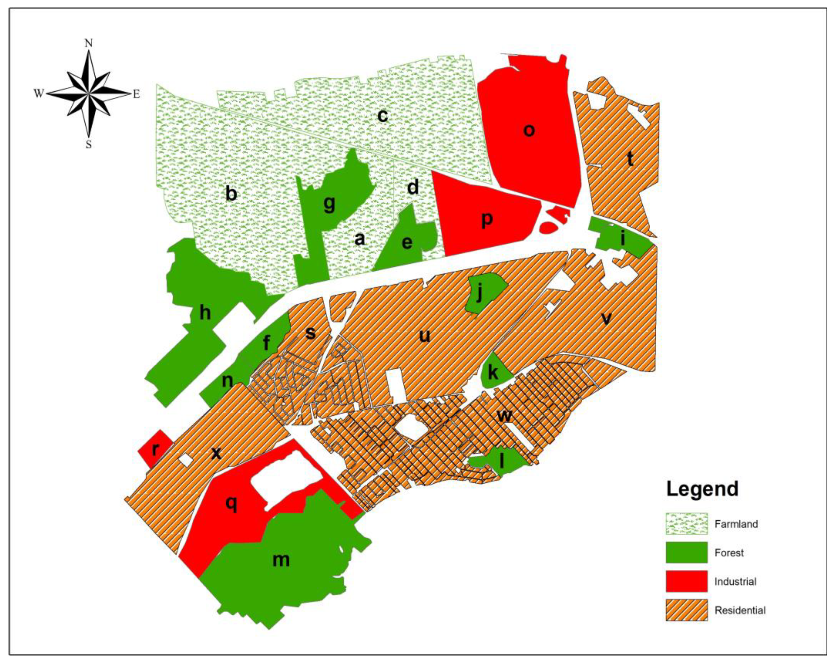
Sainte-Marthe-sur-le-lac covers an area of approximately 32 km². The area is divided into segments, each identified with a letter, based on land coverage (Figure 4). A semi-variogram was locally computed for every segment and a theoretical model was fitted to each semi-variogram for the corresponding segment. Then, the coefficients values were measured through the fitted model for farmland, forest, industrial, and residential areas (

Table 1. Overview of the coefficients obtained from the fitting model for each segment.

LULC	Letter	Variance (m2)	Range (m)	Nugget (m2)
Farmland	a	0.049	19.6	0.002
	b	0.052	11	0.002
	c	0.04	11	0.002
	d	0.024	10	0.0009
	Average	0.041	13	0.0017
Forest	Letter	Variance (m2)	Range (m)	Nugget (m2)
	e	0.075	10	0.003
	f	3.4	43	0.001
	g	0.15	13	0.003
	h	0.6	26	0.002
	i	0.28	19	0.003
	j	0.037	8	0.004
	k	0.21	18	0.002
	l	0.47	16	0.000
	m	0.11	14	0.002
	n	2.6	32	0.000
	Average	0.79	20	0.002
Industrial	Letter	Variance (m2)	Range (m)	Nugget (m2)
	o	0.17	14	0.00
	p	0.12	13	0.003
	q	0.25	16	0.002
	r	0.11	16	0.001
	Average	0.16	14.7	0.0015
Residential	Letter	Variance (m2)	Range (m)	Nugget (m2)
	s	0.04	12	0.002
	t	0.19	17	0.000
	u	0.007	14	0.002
	v	0.28	22	0.000
	w	0.06	13	0.001
	x	0.21	17	0.000
	Average	0.13	15.8	0

).

As depicted in Table 1, the variance changed markedly across the region. All segments fitted well to a bounded model; thus, there was no need for a trend model and ordinary kriging was appropriate in these cases [14]. The other key point of all fitted models is the concavity around the origin, which may be either smooth or curved. This implies local variation across the region, as demonstrated by the example of neighboring segments s and f. Segment s has a very small variation, whereas segment f shows higher variation, illustrating that the stationary or global variogram may not be an adequate representation of spatial variability.

Based on the results, the variance of farmland was minimal, ranging from 0.04 to 0.052 m². This suggests that farmland LULC is typically flat with minimal features; thus, we anticipate a consistent amount of error for this LULC. In forests, the variation of variance was significantly higher compared to farmland, ranging from 0.037 to 3.4 m². This large variance is attributed to the varying densities of trees and the local environments in which the forest is situated. For example, segment g, located between segments a and b, has a considerably smaller and more similar variance due to its proximity to farmland segments. Similarly, segments j and k have smaller variances due to their proximity to residential areas.

Segments (o–r) and (x–s) correspond to industrial and residential LULC, respectively, with variances ranging from 0.11 to 0.25 m² and 0.04 to 0.28 m², respectively. The minimum variance in residential areas was lower than that of industrial segments. It is worth noting that it may be possible to observe the same variance between different types of LULC, but the question is if the same error exists. Neglecting the nugget value, the range is the key value to determine which LULC produces the higher error. We expected a higher error in the model with a lower range, as the fitting model would level out at a lower distance. For example, although segment v with residential LULC and segment i with forest LULC had the same variance, the distance where the model flattened out for the former was longer than for the latter (range i = 19.2 m: range v = 22.4 m). Thus, we anticipate a lower error in residential compared to forest LULC. The average variances of the residential and forest areas are shown in Table 1.

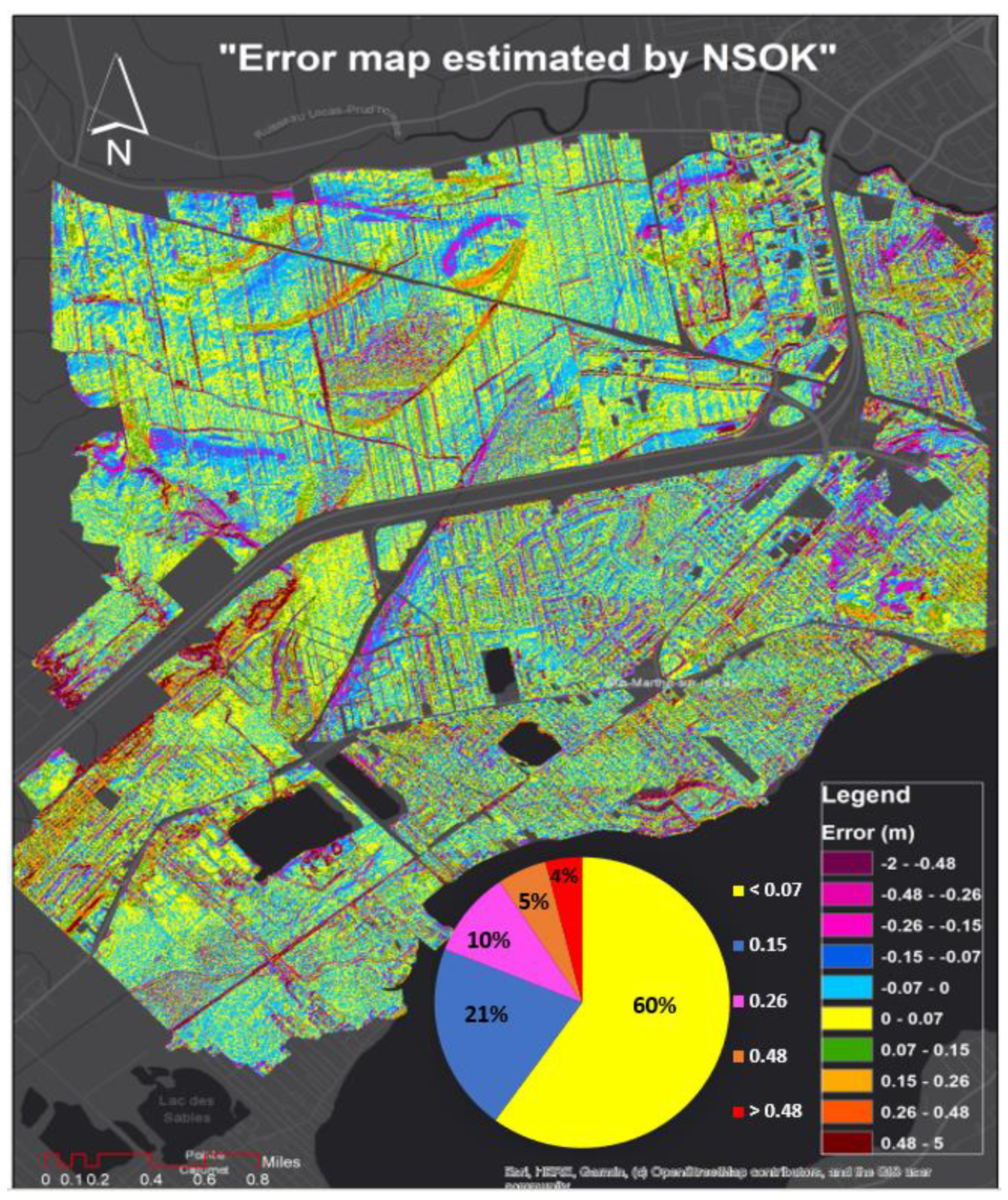
The error map obtained via NSOK is illustrated in Figure 5. This map displays the elevation error for every 5 m distance, with the error ranging from −5 to 5 m. In addition, it reveals the percentage of error in different intervals. Analysis of the circular diagram demonstrates 60% of the cells contained an error of less than 7 cm. Additionally, 21%, 10%, and 5% of cells had an absolute error of (7–15), (15–26), and (26–48) cm, respectively. Lastly, less than 5% of cells contained an error of more than 48 cm.

Even after excluding the main roads from our computation, the primary sources of these large errors arose from roads that traversed through the forest or residential areas. The dense trees adjacent to the buildings were also a contributing factor. Additionally, we sometimes observed small forests or clusters of trees located in the middle of residential areas or farmland, which was not classified as separate LULC. This is another source for the large errors, particularly in residential or farmland, and even industrial LULC. This leads to the fact that there is sometimes not a distinct boundary between LULCs.

4.1.1. Comparison with OK

In this section, we aim to evaluate the performance of the NSOK against the stationary method.

For this purpose, the stationary variogram was computed for Sainte-Marthe-sur-le-lac. Similarly, to the non-stationary variogram modeling, a Gaussian model was fitted to the experimental variogram. Then, variance, range and nugget values of 0.14 m², 16.4 m and 0.002 m² were computed, respectively.

OK only allows us to compute a single set of parameters, because it supposes the spatial variability is stationary. Conversely, examination of the non-stationary variogram uncovered considerable spatial variation across the entire region (Table 1). Indeed, the NSOK method provided the flexibility to calculate distinct parameter sets for various LULC, offering a localized perspective.

To make a comparison between these two methods, we delved into further assessment by estimating the elevation error and subsequently calculating the RMSE for both methods. This analysis not only highlighted the variance differences but also provided a robust evaluation of their respective performances. The visual representation of the differences in RMSE is presented in Figure 6. By analyzing the statistical results, we observed that the lowest RMSE value was obtained for farmland at 19 cm, followed by residential areas at 25 cm, which was equal to the average RMSE value obtained from the stationary method. The maximum error obtained corresponded to the forest area at 41 cm, which was higher than the average stationary result. The estimated error for industrial areas was approximately 33 cm, which was slightly higher than average. Our results indicate that a stationary variogram is insufficient to effectively describe the spatial variability in a single spatial model; however, the NSOK reflects the spatial variability of terrain more accurately (Figure 6).

4.1.2. Comparison with GT

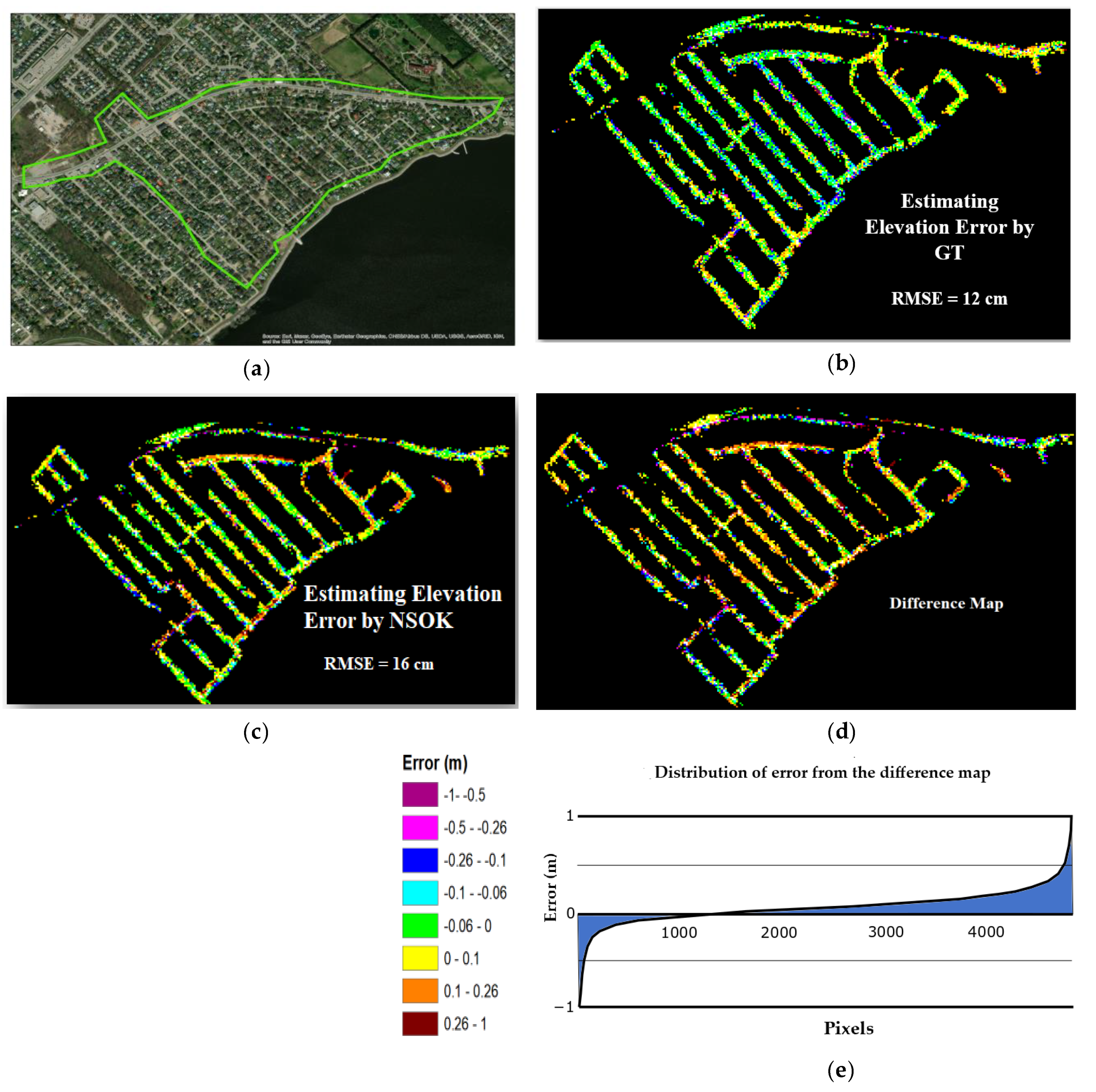
To evaluate the effectiveness of the NSOK technique, we carried out a practical comparison with a GT method, a commonly used approach for assessing the accuracy of LiDAR point clouds. As we mentioned earlier, the method relies on terrestrial LiDAR data collected by an external company and used as a GT. However, it is important to note that these data only cover specific areas along the streets of Sainte-Marthe-sur-le-lac, rather than the entire town. To make this comparison between NSOK and GT meaningful, we chose a specific zone where we had access to GT elevation error measurements. This allowed us to assess how well NSOK performs in comparison to the traditional GT method (Figure 7a). The accuracy estimated using the GT yielded a better estimation of the error (Figure 7b,c). The average RMSE values obtained from the two methods were quite similar, with a difference of 4 cm (Figure 7d). The difference map and statistics indicated that more than 70 percent of cells had an actual and predicted error of less than 10 cm (Figure 7e). A higher disparity between the two methods was generally observed near roads.

4.2. Saint-Amable

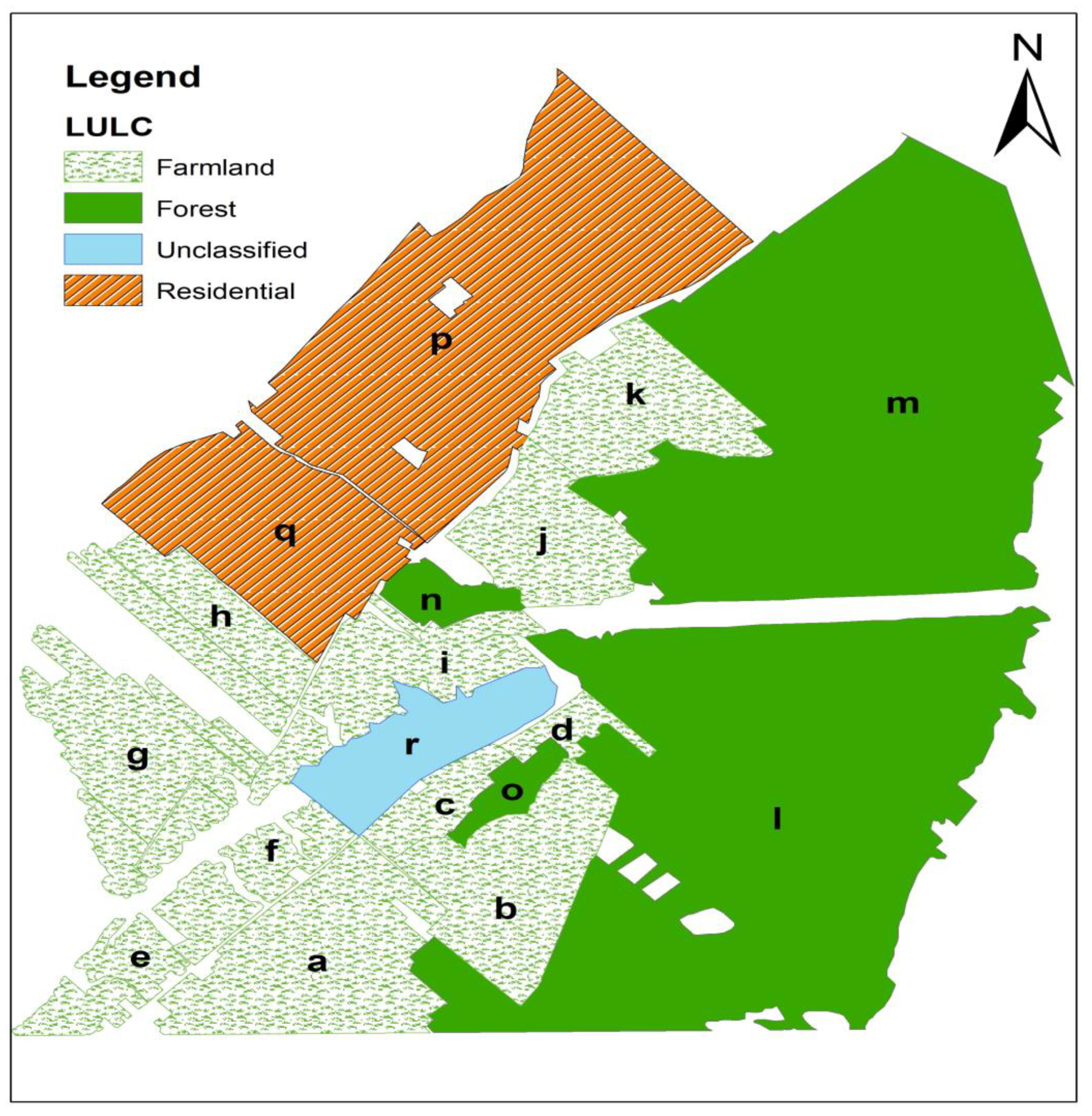
Saint-Amable was the second case study and covers an area of approximately 23 km². Like the first case study, OSM’s LULC was utilized for segmentation. This analysis was limited to residential, forest, farmland, and unclassified LULC areas (Figure 8). The coefficient values were obtained through the fitted models for the farmland, forest, and residential LULC (

Table 2. Coefficient values obtained from fitted model for each section.

LULC	Letter	Variance (m2)	Range (m)	Nugget (m2)
Farmland	a	0.018	12.6	0.0025
	b	0.10	15.14	0.0036
	c	0.035	14.1	0.0015
	d	0.018	12.6	0.002
	e	0.037	16.42	0.0012
	f	0.031	15.12	0.002
	g	0.027	16.22	0.0015
	h	0.016	10.18	0.002
	i	0.061	16	0.002
	j	0.11	17.12	0.002
	k	0.029	14.4	0.0025
	Average	0.043	14.5	0.002
Forest	Letter	Variance (m2)	Range (m)	Nugget (m2)
	l	1.87	37.32	0.0003
	m	1.35	32.34	0.0008
	n	0.328	17.72	0.0000
	o	0.089	11.4	0.0006
	Average	0.91	24.7	0.0004
Residential	Letter	Variance (m2)	Range (m)	Nugget (m2)
	p	0.047	13.04	0.0027
	q	0.060	13.4	0.0017
	Average	0.053	13.22	0.002
Unclassified	Letter	Variance (m2)	Range (m)	Nugget (m2)
	r	1.95	28.5	0

). The Gaussian model was determined to be the most suitable fitted model for the experimental variogram.

The segments (a–k) corresponded to farmland, and there was a similar range of spatial variation across most of the segments. Segments b and j, however, reflected higher variance than other segments due to their proximity to the forests and the presence of dense grass or trees in certain areas. When compared with other LULCs, the farmland demonstrated the lowest variance. The segments (l–o) related to forest LULC. The average variance in forests is significantly greater than in other LULCs. In comparison to farmland segments that demonstrated a relatively uniform spatial variation across the region, the spatial variation in forest segments was highly diverse. This variation was largely dependent on the area that the forest segment occupies, the type of tree, the densities of the trees, and its geographic location. As an example, segment o had lower variance than segments l, m, and n due to its proximity to farmland and its small area coverage. Segments p and q corresponded to the residential LULC and had similar variance. It should be noted that the variance in residential areas was higher than that of farmland, but lower than that of forest. Upon comparing the average variance, range and nugget values between different LULCs, it was found that the average nugget value of farmland and residential areas was the same; however, the average nugget value for forest was lower than the other two. Additionally, the average variance and range in the forest was longer than in the other two LULCs. The unclassified segment r had the highest variance, as evidenced by the steep slope in the middle of the segment due to the presence of a river (Table 2). Furthermore, part of this segment was covered by forest and the flat area.

The error map was obtained using NSOK, which represented the elevation error for every 5 m distance (Figure 9). The corresponding circular diagram demonstrates the percentages of error in different intervals. It is evident that the error ranged from −3 to 3 m. Analysis of the diagram reveals that 59% of the cells had an error of less than 7 cm, and 20%, 9%, and 6% had absolute errors of (7–15), (15–26), and (26–48) cm, respectively. Finally, 6% of the cells contained an error of greater than 48 cm. The significant errors that occurred in the middle and left edge of the map belonged to the forest (Figure 9). Upon further investigation, it was determined that the errors were caused by the mainstream passing through the middle of the city and the tributary that sometimes feeds into it. The variation in slope in the middle and left edge of the map was identified as another contributing factor to the errors (Figure 10). A comparison of Figure 9 and Figure 10 reveals that the error map reflects the variation of the slope.

4.2.1. Comparison with Ordinary Kriging

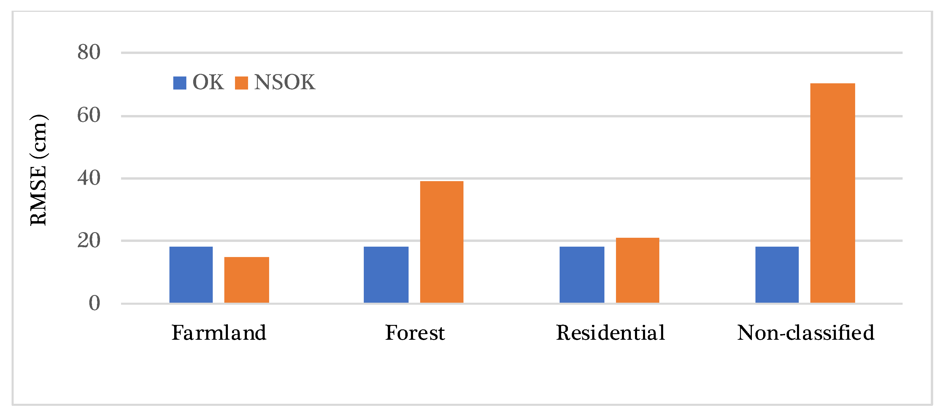
In this section, we intend to compare NSOK against OK. To make a comparison, we delved into further assessment by estimating the elevation error and subsequently calculating the RMSE for both methods. The comparison between the two methods revealed that farmland was the only LULC for which the RMSE was lower than the average RMSE obtained using the stationary method. The residential RMSE was nearly equal to the stationary error, with a difference of 3 cm. The maximum error was associated with the forest and unclassified LULC, with RMSE values of 39 cm and 70 cm, respectively (Figure 11).

4.2.2. Comparison with GT

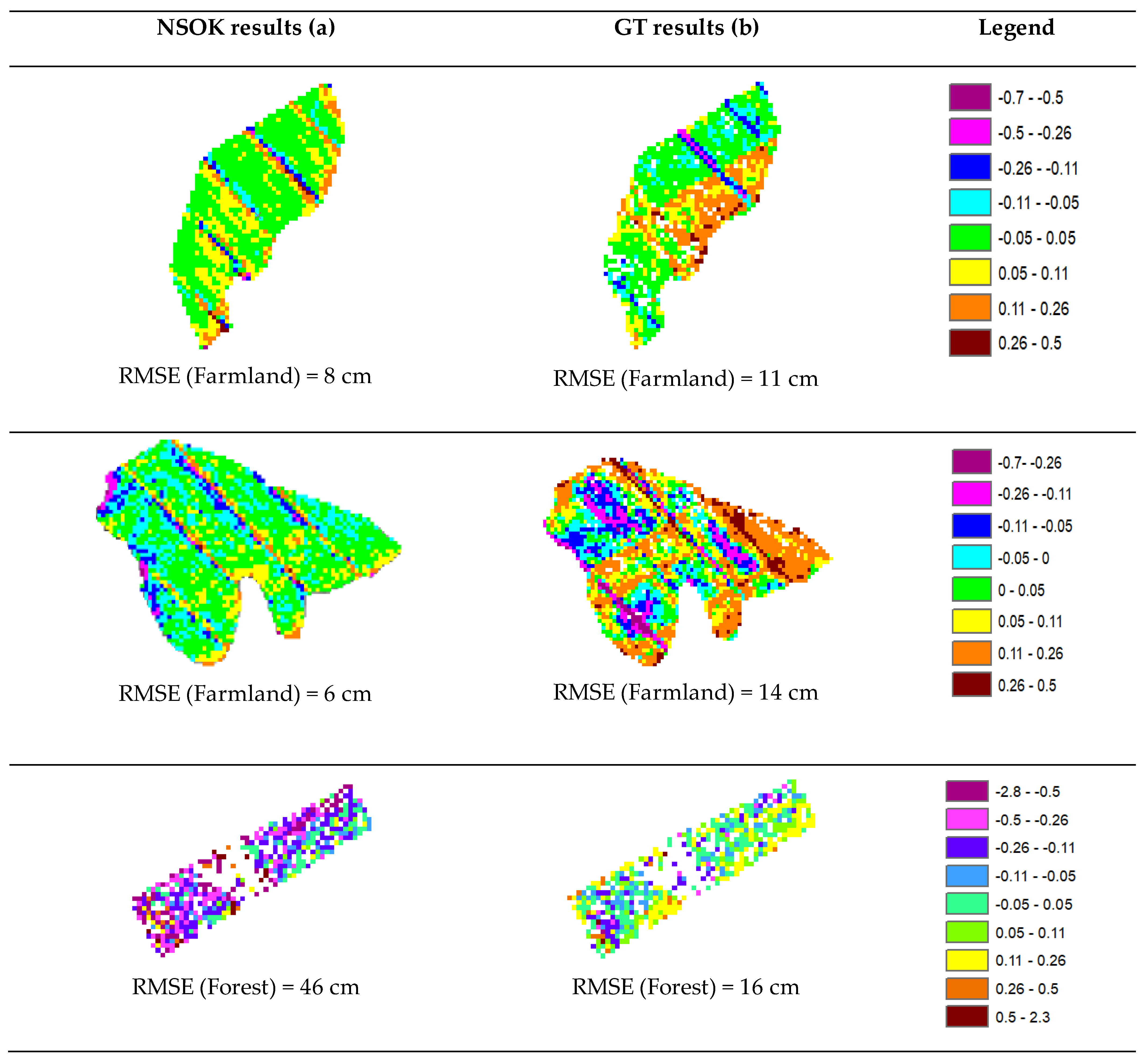
In this section, we aim to compare the results obtained using GT and NSOK. To this end, we selected two sections in farmland and one section in forest where we had results for both methods (Figure 12).

The results indicate that the RMSE value obtained in the forest for both methods was higher than what was found in farmland. Specifically, NSOK showed better accuracy than GT for farmland LULCs, whereas NSOK yielded worse results in the forest. It is worth mentioning that the higher RMSE in the forest was also observed in Sainte-Marthe-sur-le-lac, confirming that accuracy is lower in forests. In forests, the RMSE value for the GT was lower than that obtained using NSOK. This is attributed to the fact that the error estimated using GT is only affected by interpolating the four neighboring points and their distance, while the error calculated using NSOK is additionally influenced by the coefficient obtained through variogram computation (Figure 12). This effect was more pronounced in forests with steep slopes, due to the lower and inhomogeneous density of points compared to other LULCs (Figure 13). This was because the correlation between the density and LULCs indicated that the highest, medium, and lowest densities corresponded to the farmland, forest, and residential areas, respectively. Furthermore, the lowest error was found to correspond to farmland with the highest density, while the highest error corresponded to forest with the lowest density (Figure 13). In conclusion, the RMSE obtained for each LULC was highly correlated with its density.

5. Discussion

Kriging prediction relies heavily on the coefficient obtained through variogram modeling. Stationary variogram modeling provides insight into the global variation across a given region, while non-stationary variogram modeling allows for a more precise analysis of local variability. It is interesting to note that the global variance obtained in Sainte-Marthe sur-le-lac was close to the residential variance, with an average RMSE value that was equal to the residential RMSE, but higher than the RMSE value of farmland and lower than that of the industrial areas and forests. This suggests that global modeling does not accurately reflect spatial variability, whereas NSOK does. It was found that the Gaussian model was the best-fitted model for the two regions tested, thus making it the default model. This decision was reached after careful examination and testing of the experimental variogram model, highlighting the importance of human decision making for finding the most accurate coefficients. Non-stationary modeling solves the challenge of spatial-variation reflection; however, the accuracy of the coefficients obtained from these models is dependent on the model used.

The type of land use is another contributing factor that impacts the coefficient of the fitted model. In this study, the road network was excluded from the computation due to its potential to create large errors. This is because a road network is a linear feature which is converted into a polygonal feature by creating a buffer around it. The width of this feature is small, while the length is long; thus, the spatial variation is only found in the longitudinal direction. This means that the pairs of points used to compute the variance are only distributed in the longitudinal direction, leading to an inaccurate calculation of the variogram. To address this issue, an anisotropy variogram analysis should be employed.

The density of the points is another influential factor in the accuracy of the coefficients obtained from the fitted model. For instance, in forests where the density of points is typically lower and heterogeneous, the coefficients were acquired with reduced accuracy. This problem can be exacerbated in forests where part of it features a steep slope (e.g., section m in Saint-Amable).

The issue of different types of land use being difficult to clearly separate from each other was evident in the areas under our investigation. An example of this is section r in Saint-Amable, where a river runs through the middle and its edges are surrounded by forest. Therefore, the combination of two or more types of land use in one region, like segment r in Saint-Amable, increase not only the RMSE value, but also the uncertainty in the estimation of error.

In this research, the NSOK method was compared with GT in order to assess its performance in residential, farmland, and forest land use. The residential area was selected for comparison in Sainte-Marth-sur-le-lac, and the farmland and forest areas were selected in Saint-Amable. The results indicated that NSOK yielded higher accuracy in farmland, likely due to its flat terrain and lack of features. In residential areas, the accuracy of NSOK was nearly equal to that of GT, with a difference of 4 cm. Conversely, NSOK yielded lower accuracy in the forest, as the low density of points led to a lower accuracy of the coefficients obtained from the fitted model.

6. Conclusions

This paper proposed a method to estimate the elevation accuracy of an ALS point cloud in order to support decision makers in estimating the damages caused by floods at a provincial scale. This method is based on NSOK and provides an estimation of the elevation error of the LiDAR point cloud. The main benefit of this method was its independence from GT for accuracy assessment, and it was divided into three phases. First, the terrain was segmented based on LULC criteria via the OK application in each segment. Second, a mathematical model was fitted to each experimental variogram corresponding to each section to compute the demand coefficients for sampling space in kriging prediction. Lastly, OK was employed in each segment to predict a z-value, and the accuracy of the LiDAR point cloud was estimated through cross-validation. We adapted the proposed method with a K-D-tree indexing approach and Quad-Tree segmentation in order to efficiently process large datasets.

In order to evaluate the performance of NSOK, two case studies (Sainte-Marthe-sur-le-lac and Saint-Amable) were selected to compare the results with a global model. The error measurement yielded using NSOK demonstrated an improvement over the global model and could be employed as a good indicator of accuracy for decision makers. The accuracy of the point cloud in farmland and residential areas was either equal to or better than the global model, while in the forest and industrial areas, it was lower than the global model. Consequently, we can infer that the global model may not accurately reflect the geographic variations across different LULC types. We validated the reliability of NSOK by comparing it to the GT in areas where access to the GT was available. Our conclusion was that NSOK performed well, as the error measurement given by NSOK was reflective of the error measured by the GT. We observed a positive relationship between the LULC and point-cloud density. Both methods showed lower numbers of errors in farmland and residential areas, while higher numbers of errors were observed in forests. These higher number of errors indicate that the accuracy of ALS point cloud in forests is not as good as in other areas, likely due to the lower density of the point clouds in these areas. Therefore, NSOK is reliable, particularly in cases where access to high-precision third-party datasets or GT is limited.

Determining if the proposed method is a viable option for decision makers in the flood-risk-estimation field requires further examination. Although decision makers may not always provide specific accuracy requirements, they can use error maps to evaluate the accuracy of an ALS point cloud and spot areas that require more care. If urban areas are the main focus, then having higher error margins in unimportant areas may be a suitable solution. If, however, higher errors remain a concern, additional data collection may be warranted to improve accuracy in critical areas.

In this work, identifying the optimal model to fit the experimental variogram model posed a challenge and necessitated manual intervention. We conclude that the Gaussian model was the most suitable for the experimental variogram, and, thus, consider it a default model. We recommend assessing fitting models prior to utilizing NSOK in other areas.

Despite validating our approach with GT in two case studies, the limitation of this work was that GT was only located in residential areas in Saint-Marthe-sur-le-lac. Consequently, further testing of our method is necessary in other locations. In addition, to further address the accuracy of point clouds located in low-density forests, we will develop a workflow that is more adaptive to these environments in order to estimate elevation errors more accurately.