Article

A Swin Transformer with Dynamic High-Pass Preservation for Remote Sensing Image Pansharpening

College of Computer Science and Technology, Chongqing University of Posts and Telecommunications, Chongqing 400065, China
*
Author to whom correspondence should be addressed.
Remote Sens. 2023, 15(19), 4816; https://doi.org/10.3390/rs15194816
Submission received: 30 August 2023 / Revised: 29 September 2023 / Accepted: 2 October 2023 / Published: 3 October 2023
(This article belongs to the Section Remote Sensing Image Processing)

Abstract

:
Pansharpening is a technique used in remote sensing to combine high-resolution panchromatic (PAN) images with lower resolution multispectral (MS) images to generate high-resolution multispectral images while preserving spectral characteristics. Recently, convolutional neural networks (CNNs) have been the mainstream in pansharpening by extracting the deep features of PAN and MS images and fusing these abstract features to reconstruct high-resolution details. However, they are limited by the short-range contextual dependencies of convolution operations. Although transformer models can alleviate this problem, they still suffer from weak capability in reconstructing high-resolution detailed information from global representations. To this end, a novel Swin-transformer-based pansharpening model named SwinPAN is proposed. Specifically, a detail reconstruction network (DRNet) is developed in an image difference and residual learning framework to reconstruct the high-resolution detailed information from the original images. DRNet is developed based on the Swin Transformer with a dynamic high-pass preservation module with adaptive convolution kernels. The experimental results on three remote sensing datasets with different sensors demonstrate that the proposed approach performs better than state-of-the-art networks through qualitative and quantitative analysis. Specifically, the generated pansharpening results contain finer spatial details and richer spectral information than other methods.

1. Introduction

Given the inherent physical limitations of remote sensing satellite sensors, achieving imagery with both high spatial and spectral resolutions poses a significant challenge. Pansharpening has emerged as a pivotal preprocessing technique within numerous remote sensing applications. Its primary objective is to fuse multispectral (MS) imagery with panchromatic (PAN) data, ultimately yielding an MS image mirroring the spatial resolution of the PAN data. Numerous pansharpening methods have been developed in recent years, which can be roughly divided into two categories, i.e., traditional and deep learning-based.
Traditional methods mainly contain component substitution (CS), multiresolution analysis (MRA) and variational optimization (VO) techniques. In essence, the core concept behind CS methods revolves around projecting the low-resolution MS image into a compatible domain. This projection facilitates the replacement of the spatial information component within the low-resolution MS image with corresponding spatial details extracted from the PAN image. This process is undertaken while endeavouring to preserve the original spectral information to the greatest extent possible. Prominent techniques encompass intensity–tone–saturation, principal component analysis [1,2,3], Gram–Schmidt [4], adaptive component replacement method [5], etc. Moreover, the fundamental principle underlying the MRA method involves the extraction of spatial components from low-resolution MS images through a process of multiresolution decomposition. Subsequently, these spatial components are substituted with panchromatic images containing intricate high-frequency details. Representative methods include the Laplacian pyramid decomposition [6], wavelet transform [7,8] and contour wave [9] methods. In contrast, the VO-based approach capitalizes on existing prior information to formulate regular terms that effectively constrain the model. This strategy leads to the derivation of the ultimate panchromatic sharpening outcome through a streamlined solution algorithm. Noteworthy methodologies within this category encompass the construction of sparse priors for regular terms [10], the utilization of image-based nonlocal similarity [11] and the integration of fragment smoothness [12] into the regularization model. These approaches distinctly enhance the accuracy of both spectral and spatial dimensions within the model.
With the development of artificial intelligence, machine leaning methods [13,14,15] and deep learning methods have been dominant in remote sensing processing and interpretation [16,17,18,19]. Notably, convolutional neural networks (CNNs) have exhibited promising performance [20,21,22,23] owing to their adeptness in uncovering abstract features within remote sensing imagery. Their robust prowess in image reconstruction further contributes to their efficacy in this context. CNN-based pansharpening can be conceptualized as an image fusion and reconstruction network, trained in an end-to-end manner. The existing approaches can be categorized into five distinct frameworks, as illustrated in Figure 1.
The CNNs essentially attempt to extract deep representations of PAN and MS images and reconstruct high-resolution images while preserving spectral information. Recently, residual learning has been a popular choice in pansharpening networks due to its effectiveness in supplementing spectral information, as shown in Figure 1b–d. However, various detail injection paradigms exist because they adopt different convolutional networks with different detail injection and spectral preservation approaches. As shown in Figure 1, the interactions between the PAN and MS encompass concatenation [24], subtraction [25] and addition [26]. Residual blocks with shortcuts or skip connections have been utilized to ensure the input information can be sufficiently propagated through all layers. They can also effectively relieve the phenomenon of gradient disappearance and explosion. On this basis, numerous efforts have been made to improve the representation capability of CNNs, such as dual-branch CNN [27], local-context adaptive kernels [24], subpixel convolutional layers [27] and multiscale convolutions [26].
More recently, generative adversarial networks (GANs) have been introduced into pansharpening [28,29,30,31,32], using a discriminator to distinguish the generated high-resolution images from the ground truth. Although adversarial training can improve the discriminative capability of the pansharpening network, some fake textures could inevitably be produced.
In addition, some algorithm-unrolling-based networks have been proposed [33,34,35]. Such methods assume the prior distribution between the HR target image and the HR guidance image, and they use one or two algorithms to solve the loss function or optimization function. Eventually, the algorithm is unrolled into a deep learning network, which has the benefit of making the model more interpretable.
While CNN-based approaches have demonstrated remarkable performance compared to conventional methods, they still grapple with the inherent limitations of CNN networks, including their relatively short-range interactions and restricted receptive fields. This can lead to challenges in effectively preserving spatial details, ultimately resulting in notable spatial detail loss within the high-resolution MS images produced by these CNN networks.
Recently, self-attention-based transformer models have been used to model the long-distance dependencies of different pixels within feature maps [36]. They are conducive to capturing vital contextual information from remote sensing images for recovering high-resolution MS images [37,38,39,40]. The MS and PAN images are stacked directly or fed into a two-branch network to encode MS and PAN images and learn their interactions for the reconstruction of high-resolution fused images. However, they focus on global representations but still suffer from a weak capability to recover high-resolution detailed information.
In this paper, a framework named SwinPAN with a detail reconstruction network (DRNet) is proposed to reconstruct high-resolution spatial and spectral details from input images. The process of obtaining the fused image revolves around incorporating the high spatial structures from a high-resolution PAN image into a resampled MS image. These high spatial structures are typically derived from the difference between the HR PAN and low-resolution (LR) components. A more in-depth exploration is conducted by directly feeding the network with details extracted through the differentiation of the individual PAN image with each MS band.
In summary, the main contributions of our work are as follows.
  • The detail injection mechanism is further investigated in pansharpening networks. A dynamic high-pass preservation module is developed to enhance the high frequencies present in input shallow features. This module achieves its objective by adaptively acquiring the expertise to generate convolution kernels. Furthermore, it strategically employs distinct kernels for each spatial location, facilitating the effective amplification of high frequencies.
  • A subtraction framework with details directly extracted by differentiating the single PAN image with each MS band is proposed. This solution allows us to avoid compromising the spatial information with a preprocessing step using detailed extraction techniques proposed in classical pansharpening approaches, letting the framework spectrally adjust the extracted details through the estimation of the nonlinear and local injection model.
  • A full transformer network named SwinPAN is developed for pansharpening based on the Swin Transformer. The proposed network introduces content-based interactions between image content and attention weights, resembling spatially varying convolutions. This is achieved through a shifted-window mechanism, which enables effective long-range dependency modelling. Notably, the Swin Transformer boasts improved performance while utilizing fewer parameters in comparison to the Vision Transformer (ViT).
  • Experimental results on three remote sensing datasets, including QuickBird, GaoFen2 and WorldView3, demonstrate that the proposed method achieves superior performance competitiveness compared with other state-of-the-art CNN-based methods.

2. Related Works

2.1. CNN-Based Methods

PNN [41], as the first CNN-based pansharpening model, took a three-layer- convolutional network adapted from SRCNN [42] as its backbone. More specifically, the PNN upsamples a low-resolution MS image to the size of the PAN image. Then, the upsampled image is concatenated with the PAN map along the channel dimension to form the input of the network. Although PNN has fewer network parameters, it converges relatively slowly due to the simple network structure. The DiCNN [43] method first concatenates the PAN map and the upsampled low-resolution MS map. The convolutional layer is used to learn the residual details of the image, and, finally, the output of the network is directly added to the upsampled low-resolution MS image to obtain the final fused image output. Skip connections were adopted to alleviate gradient explosion and speed up the convergence of the network. Furthermore, PanNet [44] attempts to split the panchromatic sharpening task into two objectives: structural and spectral preservation. For structural preservation, detailed contents obtained via the high-pass filter are fed into the CNN. For spectral preservation, PanNet directly adds the upsampled MS map to the output of the spatial detail learning network, which can effectively propagate the spectral information directly to the output image. For MSDCNN [26], the authors designed convolution kernels of different sizes to extract features with different scales and receptive fields, thereby enhancing the network’s representation ability. For BDPN [26], the authors designed a pyramid-based bidirectional network architecture to process low-resolution MS maps and high-resolution PA maps, respectively. Through this network, the multiscale details of the PAN map can be effectively extracted and injected into the MS map to obtain high-resolution output. Specifically, the entire network structure is converted between different scales. The network for extracting details uses several classic residual network blocks and the network for reconstructing images uses subpixel convolutional layers to upsample MS images. FusionNet [25] directly uses the difference between the original upsampled MS image and the PAN image to extract image details. This method can effectively maintain the spatial information and potential spectral information of the image. The extracted details are input to several residual network blocks for feature extraction and detail learning, and the final output is added to the upsampled MS map to obtain a fused image. A convolution module named LAGConv [24] that can adapt to local content is proposed, which mainly includes local adaptive convolution kernel generation and a global bias mechanism. The local adaptive convolution kernel is generated by multiplying the traditional convolution kernel with a learnable adaptive weight matrix. The global bias mechanism mainly supplements the global information loss problem caused by the previous local adaptive convolution, which is also implemented through two fully connected networks.
Although these networks have improved image reconstruction quality, it is challenging to obtain position-independent global information, and they could not make full use of intrinsically similar textual information in images.

2.2. Transformer-Based Methods

Self-attention-based transformer models have been a popular choice in pansharpening. For example, Meng et al. [37] utilized a Vision Transformer [45] for pansharpening, in which MS and PAN are stacked together and then cropped into patches to reduce the sequence length. Therefore, the pansharpening tasks can be regarded as the image fusion and reconstruction process. However, the Vision Transformer is weak in extracting multiscale contextual information. In [38,39,46], CNN and transformer encoders are conducted directly on the stacked MS and PAN images to exploit local and nonlocal features, respectively. Some works exploit two-branch structures to encode MS and PAN images separately, in which convolution and transformer modules are combined to explore spatial–spectral features [47,48]. The generated features are then fused for the reconstruction of the pansharpening image [40]. Recently, Swin Transformer [49] has drawn attention to image restoration. It uses a hierarchical structure to extract information at different scales and develops a window-based self-attention mechanism to reduce computational costs. It focuses on content-based interactions between image content and attention weights, which can be interpreted as a spatially varying convolution within a local window. Therefore, the Swin Transformer has linear computation complexity to the image size.
Although these transformer-based models have improved their performance in fetching global representations, they are limited in recovering high-resolution detailed information from abstract representations. In these models, pansharpening is regarded as a feature fusion task of MS and PAN images. The high-frequency information in the PAN image cannot be well preserved in the representation learning and image reconstruction process.

3. Methodology

3.1. Framework

As shown in Figure 2, the proposed approach adopts a subtraction framework with a DRNet to reconstruct the high-resolution spatial information and a residual module to preserve the spectral information.
Pre-processing. The MS and PAN images captured by the satellite are denoted as I M S R h × w × C i n and I P a n R H × W × 1 , respectively. The low-resolution MS image is upsampled to the same size as the PAN image. For the PAN image, it is duplicated in the channel dimension so that it has the same channels as the MS image. The images after pre-processing are denoted as I L M S R H × W × C i n and I P A N R H × W × C i n , respectively. After that, high-frequency spatial structures are obtained from the difference between the PAN and MS components as
F S U B = H S U B ( I P A N , I L M S )
where F S U B R H × W × C i n represents the generated image with spatial structures and H S U B ( · ) denotes matrix subtraction for two inputs.
Shallow feature extraction with high-pass preservation (SFE-HP). Rather than directly using F S U B as the input of the network, a dynamic high-pass preservation module is developed to retain the image’s spatial structure in the shallow features. Generally, the same weight is used in convolution operation, which is called weight sharing. However, when a low-pass filtering convolution kernel is used to check image edges, it will make the edges flatter so that it will lose spatial information. In the high-pass module, different convolution kernels are generated for each pixel, as shown in Figure 3.
As different channels will contribute different spatial information, the feature map is parted into several groups to better obtain the spatial information. This operation is also used in channel attention. The feature map is not divided into one channel for each group. Instead, the feature map is divided into several channels for each group in order to accelerate the training speed. Firstly, feature maps are divided into g groups in the channel dimension, and each group can be presented as X i , where i = 1 , 2 , , g . For each group, one convolution kernel map is generated as
w i = G ( X i ) i = 1 , 2 , , g
where G ( · ) is a function to generate different convolution kernels. G ( · ) contains four sub-modules: a convolution module, batch normalization modules, a softmax module and an invert module. The structure of the G ( · ) module is shown in Figure 3. The invert module is added to obtain the high-pass information. Otherwise, G ( · ) will obtain the low-pass information. w i presents the convolution kernel map for each group. Usually, one feature map corresponds to one convolution kernel, which is called weight sharing. In the high-pass module, different convolution kernels with dynamic variable parameters are generated for each pixel. Each kernel has K 2 parameters. These parameters are all can be trained. w i is convolved with X i R H × W × C i n g to obtain F H P i R H × W × C i n as
F H P i = H H P ( X i , w i ) i = 1 , 2 , , g
where H h p ( · ) performs the convolution operation. Lastly, g groups of F H P i are added into F H P in the channel dimension.
The shallow feature extraction is essentially a convolution layer. It is normal to add a convolution layer before the transformer model. It not only leads to stable optimization and better results but also provides a simple way to map the input space to a higher dimensional feature space. A 3 × 3 convolution layer H S F ( · ) is used to realize shallow feature extraction F 0 R H × W × C from F H P as
F 0 = H S F ( F H P )
where C is the feature channel number.
Deep feature extraction. A more complex network is used to extract spatial information. As shown in Figure 2, the input of DRNet is low-resolution high-frequency (LR-HF) features. The image is blurry at this point because it just subtracts from PAN and upsamples MS, without spatial feature extraction. After the DRNet extracts the spatial features of LR-HF features, the high-resolution high-frequency (HR-HF) features will be output. The image resolution is higher at this point.
Deep feature F D F R H × W × C is extracted from F 0 as
F D F = H D F ( F 0 )
where H D F ( · ) is the deep feature extraction module. It contains K DRNet blocks (DRB) and adds a 3 × 3 convolutional layer at the end of the module. Intermediate features F 1 , F 2 , F 3 and the deep feature extraction module’s output F D F are extracted by the block as
F i = H D R B i ( F i 1 ) , i = 1 , 2 , , K
F D F = H C O N V ( F K )
where H D R B i ( · ) and H C O N V donote the i-th DRB and the last convolution layer, respectively. Using a convolution layer at the end of the module can bring the inductive bias of the convolution operation into the transformer-based network, and lay a better foundation for the later image reconstruction of the shallow and deep features.
Image reconstruction module. The F E N D R H × W × C image is constructed by aggregating shallow and deep features as
F E N D = H C O N V ( F S U B + F D F )
where H C O N V is essentially a 3 × 3 convolution layer. It can reconstruct the image from abstract features F S F and F D F , which are the output of shallow and deep feature extraction modules, respectively.
Spectral information preservation The high-pass modules, shallow feature extraction module and deep feature extraction module are aimed at extracting the spatial information, which contains both marginal and detailed information. As for the spectral information, a residual connection is used:
I H R M S = H A D D ( I L M S , F E N D )
where H A D D ( · ) performs matrix addition.

3.2. Detail Reconstruction Block

As shown in Figure 1, the residual Detail Reconstruction Block (DRB) consists of several Detail Reconstruction Layers (DRLs) with a convolution layer. Given the features F i output by the i-th DRB, the intermediate features F i , 1 , F i , 2 , , F i , L are extracted by L DRLs as
F i , j = H D R L i , j ( F i , j 1 ) j = 1 , 2 , , L
where H D R L i , j ( · ) is the j-th DRL in the i-th DRB. A convolution layer is added before the residual connection, and the output of i-th DRB is formulated as
F i , o u t p u t = H C O N V i ( F i , L ) + F i , 0
where H C O N V i ( · ) is the last convolution layer in the i-th DRB.

3.3. Detail Reconstruction Layer

Self-attention in nonoverlapped windows. The Detail Reconstruction Layer (DRL) is based on multihead self-attention. For a given input F i , j R W × H × C , the DRL first reshapes the input to H × W M 2 × M 2 × C tensor by performing window partition, which aims to part the input into nonoverlapping M × M local windows, and H × W M 2 is the number of windows. The original multihead self-attention is computed in each window. For each feature X R M 2 × C in each window, the q u e r y ( Q ) , k e y ( K ) and v a l u e ( V ) are obtained as
Q = X · P Q , K = X · P K , V = X · P V ,
where P Q , P K , P V are projection matrices that are shared among each window. Now, the muti-head self attention is computed as
A t t e n t i o n ( Q , K , V ) = S o f t m a x ( Q K T d + B ) V
where B is a learnable relative position bias. This process is shown in Figure 4. Following this, this function is repeated h times, and the result after h times is the output of W-MSA. As for the MLPs (multilayer perceptrons), a network with two fully connected layers is contributed. Each fully connected layer will follow a GELU for further feature transformations.
Shifted-window partitioning in successive layers. Patch merging between each DRB is not used like in most other pansharpening methods to preserve spatial information as much as possible. However, this leads to a lack of communication between different windows. So, the shifted-window partition method is used, which alternates between two partitioning configurations in consecutive STLs, as shown in Figure 4.
As shown in Figure 4, the upper module uses the original window partition method (W-MSA), and the lower module uses the shift window partition method (SW-MSA). The original window partition method parts the 8 × 8 feature map into four windows whose size is 2 × 2 . For the shifted-window partition method, each window is moved to the lower right corner by [ M 2 , M 2 ] pixels from the original window, the empty pixel in the lower right corner is filled in with the upper left corner as shown in Figure 2 and masked (S)W-MSA is also used when computing self-attention.
With the alternating operation of the original window partition method and shifted-window partition method, the two successive DRNet layers are computed as
x ^ l = W M S A ( L N ( x l 1 ) ) + x l 1 , x l = M L P ( L N ( x ^ l ) ) + x ^ l
x ^ l + 1 = S W M S A ( L N ( x l ) ) + x l , x l + 1 = M L P ( L N ( x ^ l + 1 ) ) + x ^ l + 1
where x i and x ^ i denote the output feature output by the (S)W-MSA module and the MLP module in the j-th DRL, respectively, and MSA ( · ) and SW-MSA ( · ) denote the original window partition method and shifted-window partition method, respectively.

4. Experiments

4.1. Datasets

Three large-scale remote sensing datasets are employed for the evaluation of the proposed approach on pansharpening.
The WorldView-3 dataset predominantly consists of panchromatic and multispectral images comprising eight bands. These images were captured by WorldView-3 satellites within the visible and near-infrared spectral ranges. Notably, the sampling intervals for the panchromatic and multispectral images are 0.3 m and 1.2 m, respectively. This results in a spatial resolution ratio of 4 between them.
The GaoFen2 dataset comprises panchromatic images and multispectral images encompassing four bands. These images were acquired by the Gaofen2 satellite in the visible and near-infrared spectral ranges. The spatial sampling intervals for panchromatic and multispectral images stand at 1 and 4 m, respectively. This spatial difference results in a spatial resolution scale of 4.
As for the QuickBird dataset, it contains panchromatic images and multispectral images encompassing four bands. These images were captured by the QuickBird satellite within the visible and near-infrared spectral ranges. The spatial sampling intervals for the panchromatic and multispectral images are 0.61 m and 2.44 m, respectively. This results in a spatial resolution scale of 4.

4.2. Experimental Settings

4.2.1. Data Preparation

It should be noted that real-world, ideal high-resolution multispectral (MS) images are not commonly available. Hence, training samples are often acquired following Wald’s protocol. The process begins by filtering the image block using the modulation transfer function (MTF) tailored to the specific satellite. Subsequently, the nearest interpolation method is employed to downsample the image block by a specified resolution factor. This results in the creation of both panchromatic and multispectral image blocks on a lower resolution scale. Further, a 23-tap polynomial interpolation is implemented to achieve the upsampling of the multispectral image blocks. The original MS image blocks, prior to downsampling, are utilized as the reference ground truths in this context.
All PAN, MS and ground truths were cropped into patches with the size 64 × 64 , 16 × 16 and 64 × 64 , respectively. Regarding the QuickBird dataset, it comprises a total of 17,139 pairs of MS and PAN images for training purposes. Additionally, 20 image pairs are allocated for testing. Similarly, for the GaoFen2 dataset, there are 19,809 pairs of MS and PAN images available for training, along with 20 images set aside for testing and validation. Furthermore, the WorldView-3 dataset encompasses 9714 pairs of MS and PAN images designated for training. Alongside this, there are 20 images designated for both testing and validation purposes.

4.2.2. Implementation Details

For the proposed model, the stochastic gradient descent optimizer Adam was chosen for network training. The learning rate and the mini-batch size were set to 3 × 10 4 and 32, respectively. The numbers of DRBs, DRLs, attention heads and feature dimensions in each DRL are displayed in Table 1. Furthermore, the parameters of the compared methods were set following the corresponding original articles. All experiments were implemented on the PyTorch platform under the Ubuntu operating system with NVIDIA GeForce RTX 3090 graphics cards.

4.2.3. Metrics

For reduced-resolution tests, four commonly used indices were employed, including spectra mapper angle (SAM) [50], Erreur Relative Globale Adimensionnelle de Synthèse (ERGAS), spatial correlation coefficient (SCC) [51] and the multiband extension of the Universal Image Quality Index, denoted by Q 2 n [52], where Q4 represents four-band images and Q8 represents eight-band images. Specifically, SAM evaluates spectral distortions in resulting images compared with the ground truth. ERGAS represents the relative global dimensional synthesis error, while SCC evaluates the similarity of the spatial details between the results and the ground truth. Furthermore, Q 2 n is a composite measure comprising various factors to encompass correlations, the mean of each spectral band, intraband local variance and the spectral angle. Consequently, it incorporates both intraband and interband distortions within a unified index.
In the full-resolution evaluation, due to the lack of reference images, three popular nonreference indices, including D λ , D s and the quality with no reference (QNR) [53], were used. Specifically, D λ is a spectral metric for the spectral distortion, while D s is used to evaluate the spatial distortion. Furthermore, QNR is a combination of D s and D λ to measure global quality without ground truth.

4.3. Comparison Analysis

The proposed approach is compared with ten state-of-the-art pansharpening methods, including GSA [54], MTF-GLP-HPM [55], SFIM [56], DiCNN, MSDCNN, DRPNN, FusionNet, PNN, PanNet and HyperTransformer. The evaluation of performance is conducted at both reduced and full resolutions.

4.3.1. Reduced-Resolution Experiment

Quantitative analysis. Table 2, Table 3 and Table 4 provide a quantitative assessment of the compared methods alongside our proposed approach across the three reduced-resolution datasets. Notably, our proposed method achieves top-tier performance across all metrics and datasets. Particularly in the case of the WorldView3 dataset, our approach demonstrates an impressive enhancement of around 25 % in the measure. Excluding our method, MSDCNN and HyperTransformer emerge as noteworthy contenders. They yield promising results, with MSDCNN clinching the best performance in metrics such as S A M , Q 4 and S C C for the QuickBird dataset, and HyperTransformer clinching the best performance in R E G A S , and its performance on other metrics is also close to MSDCNN for QuickBird. Additionally, their efficacies are supported by their dual-stream residual information enhancement structure and transformer-based structure. However, MSDCNN’s performance does not generalize effectively to the WorldView3 dataset. Among the compared methods, DRPNN showcases better performance in terms of R E G A S on the GaoFen2 datasets, as well as superior S C C on the GaoFen2 dataset. This performance is attributed to its utilization of deep residual models as the underlying architecture. With the inherent limitations of neural network representation capacity, PNN and PanNet demonstrate suboptimal performance across all three datasets. This underscores the critical role of neural networks’ expressive power in achieving favourable outcomes. Traditional methods such as SFIM, MTF-GLP-HPM and GSA achieve poor performances. Upon reviewing Table 2, Table 3 and Table 4, it is evident that our proposed approach significantly outperforms CNN-based models, reiterating its superiority.
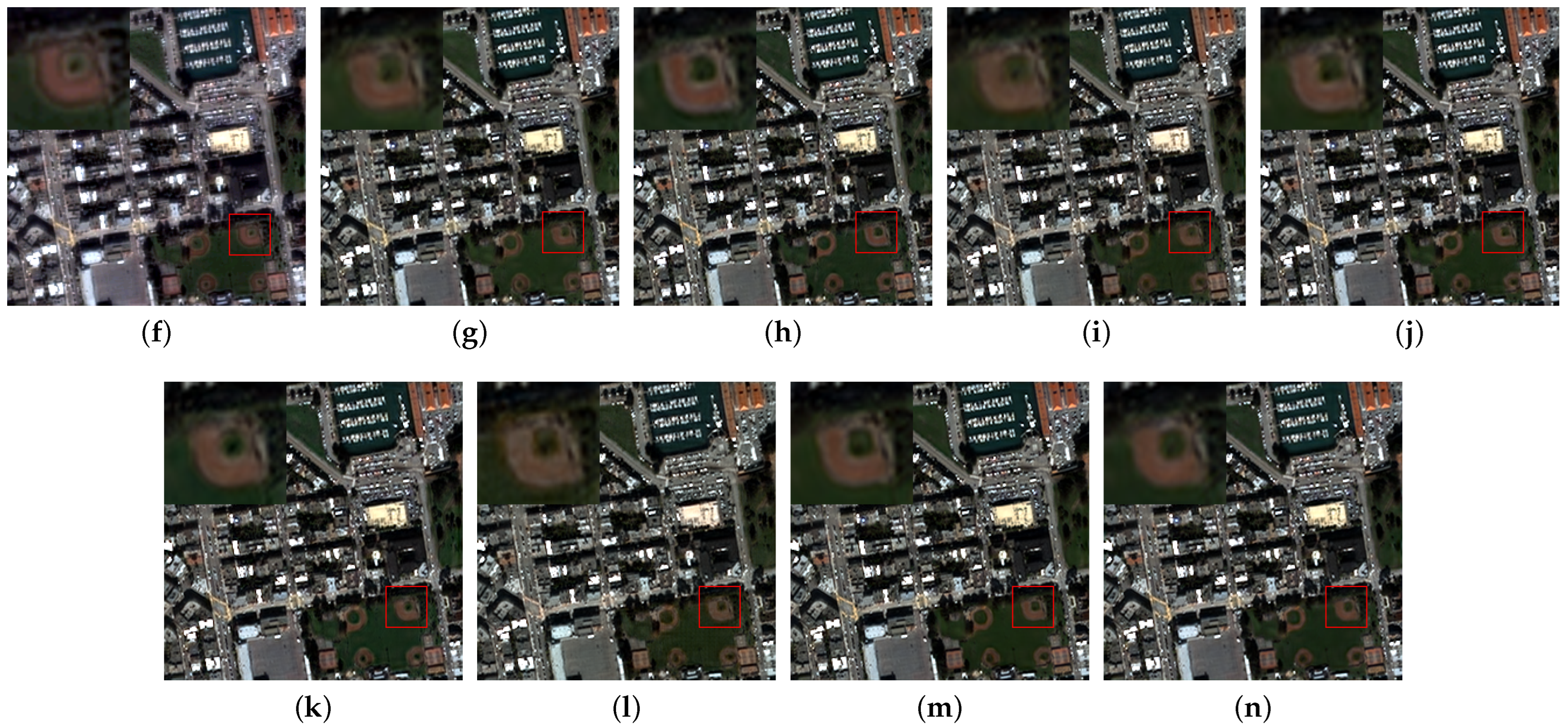
Visual comparisons. Figure 5, Figure 6 and Figure 7 provide visual insights through the comparison of sample results extracted from the test datasets. The traditional methods generally have color distortion and edge blurring among all the datasets. In the context of the QuickBird dataset, DiCNN, DRPNN and FusionNet exhibit slightly blurred edges in their outcomes. Moreover, MSDCNN, PNN, HyperTransformer and PanNet demonstrate spectral distortions. Our proposed approach, on the other hand, adeptly retains spectrum information and spatial structures. It yields outcomes featuring clean and high-frequency details that closely resemble the PAN images. Figure 6 reveals the prevalence of spectral distortions across all compared methods on the GaoFen2 dataset. Our proposed method stands out for effectively preserving spectrum information. Likewise, Figure 7 highlights spectral distortions among all the compared methods on the WorldView3 dataset. Our proposed approach maintains the bulk of the spectrum, achieving results akin to the ground-truth image. Collectively, the visual comparisons reinforce the notion that the proposed approach outperforms other state-of-the-art models.

4.3.2. Full-Resolution Experiment

Quantitative Analysis. A comprehensive evaluation is conducted of all methods using the full-resolution dataset. It is important to note that the full-resolution dataset lacks ground-truth images for testing purposes. Nevertheless, the results clearly demonstrate the superiority of our proposed method across all metrics and datasets, showcasing a substantial improvement, as shown in Table 5, Table 6 and Table 7. This underscores the robustness and strong generalization of our approach.
Among the compared methods, the traditional methods perform poorly in reconstructing high-resolution images and PNN exhibits acceptable performance on the GaoFen2 and WorldView3 datasets. However, its performance suffers on the QuickBird dataset, indicating a lack of broad applicability. HyperTransformer is also unsatisfactory in terms of model generalization; it performs well on the QuickBird and WorldView3 datasets, but suffers on the GaoFeng2 datasets. Certain methods excel in specific metrics while lagging behind in others. For instance, DiCNN performs reasonably well in terms of D λ but falls significantly short in both D s and QNR, particularly on the QuickBird and GaoFen2 datasets. This suggests that while DiCNN’s detail injection might effectively preserve spectral information, its capability to extract spatial details is constrained by the limited feature representation capacity of CNNs. MSDCNN demonstrates solid performance in the context of reduced-resolution datasets. However, this achievement does not carry over effectively to the full-resolution datasets. In stark contrast, our proposed methods consistently outperform all other approaches across all datasets, reaffirming their resilience and generalization capability.
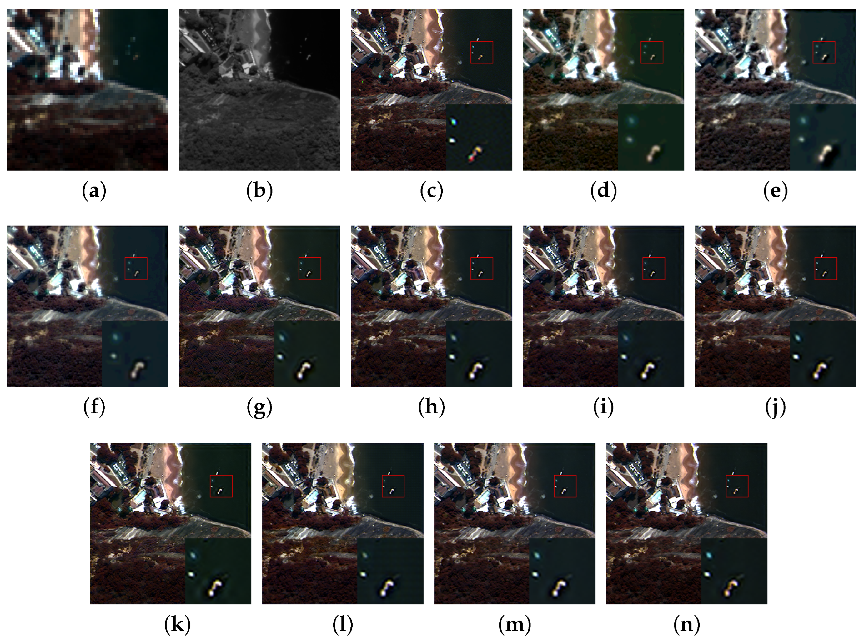
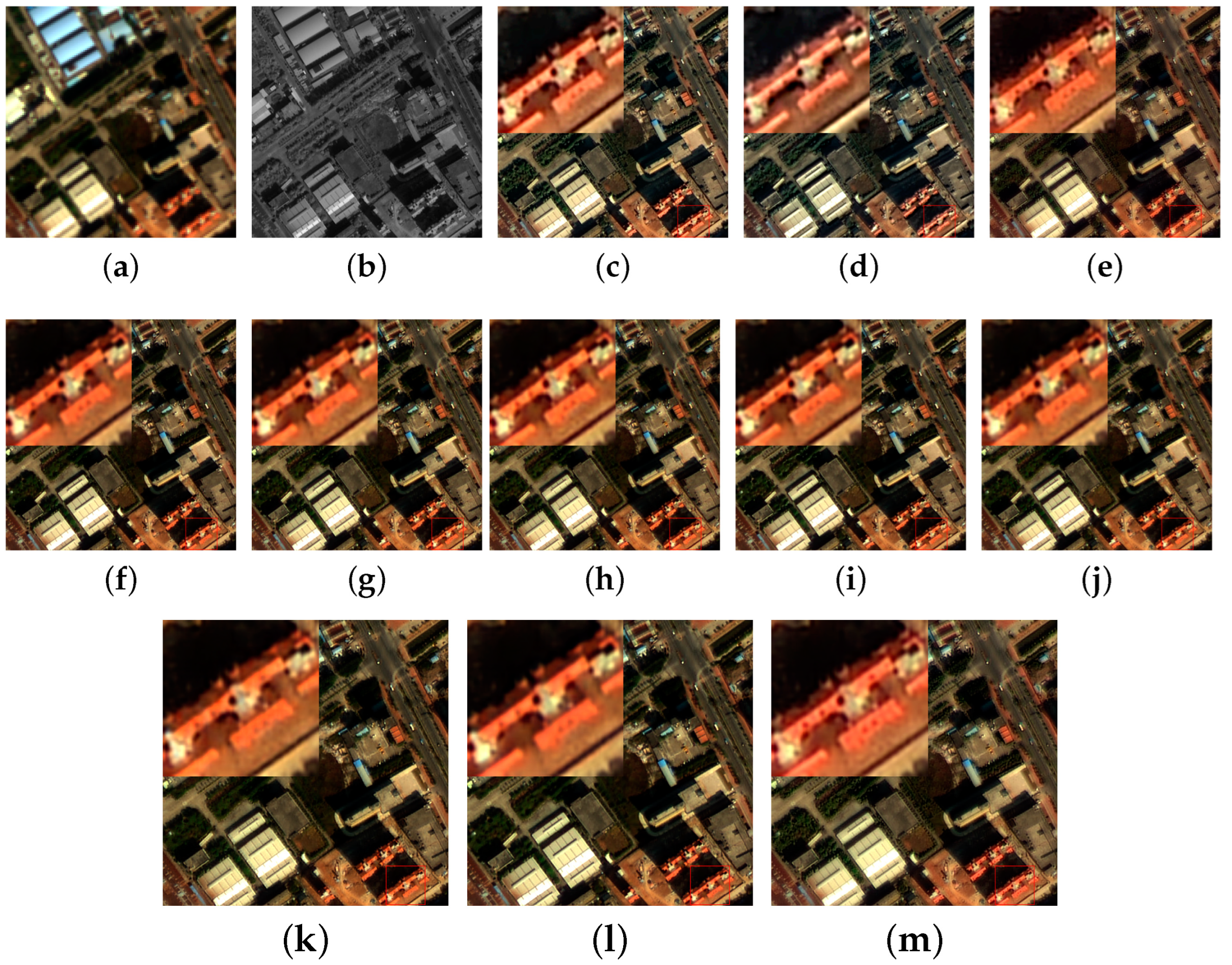
Visual comparisons. Figure 8, Figure 9 and Figure 10 visually illustrate the comparative analysis of full-resolution experimental outcomes. An important observation to note is that distinguishing visual differences among the CNN methods is not straightforward. This challenge arises from the constraints of representing the images in 8-bit RGB format, which falls short of capturing the nuances in the original 11-bit MS data. Firstly, the images generated by the traditional method have problems such as color distortion, and the blurring images have lower spectral consistency with the MS. Specifically, DiCNN, PNN, PanNet and HyperTransformer exhibit notable color distortion. Despite MSDCNN, DRPNN and FusionNet managing to retain a relatively higher amount of spectral information, they still exhibit a loss of intricate textures. Furthermore, DiCNN, MSDCNN, DRPNN and PNN result in regions of smoothing and blurring. While FusionNet, HyperTransformer and PanNet present outcomes with enhanced, detailed information and texture, they compromise spatial accuracy. In contrast, the proposed approach outperforms others by producing more precise and coherent outlines of ground objects. This is indicative of better texture information extraction and reconstruction in our method.

5. Discussion

5.1. Ablation Study

5.1.1. Albation Study of Dynamic High-Pass Preservation Module

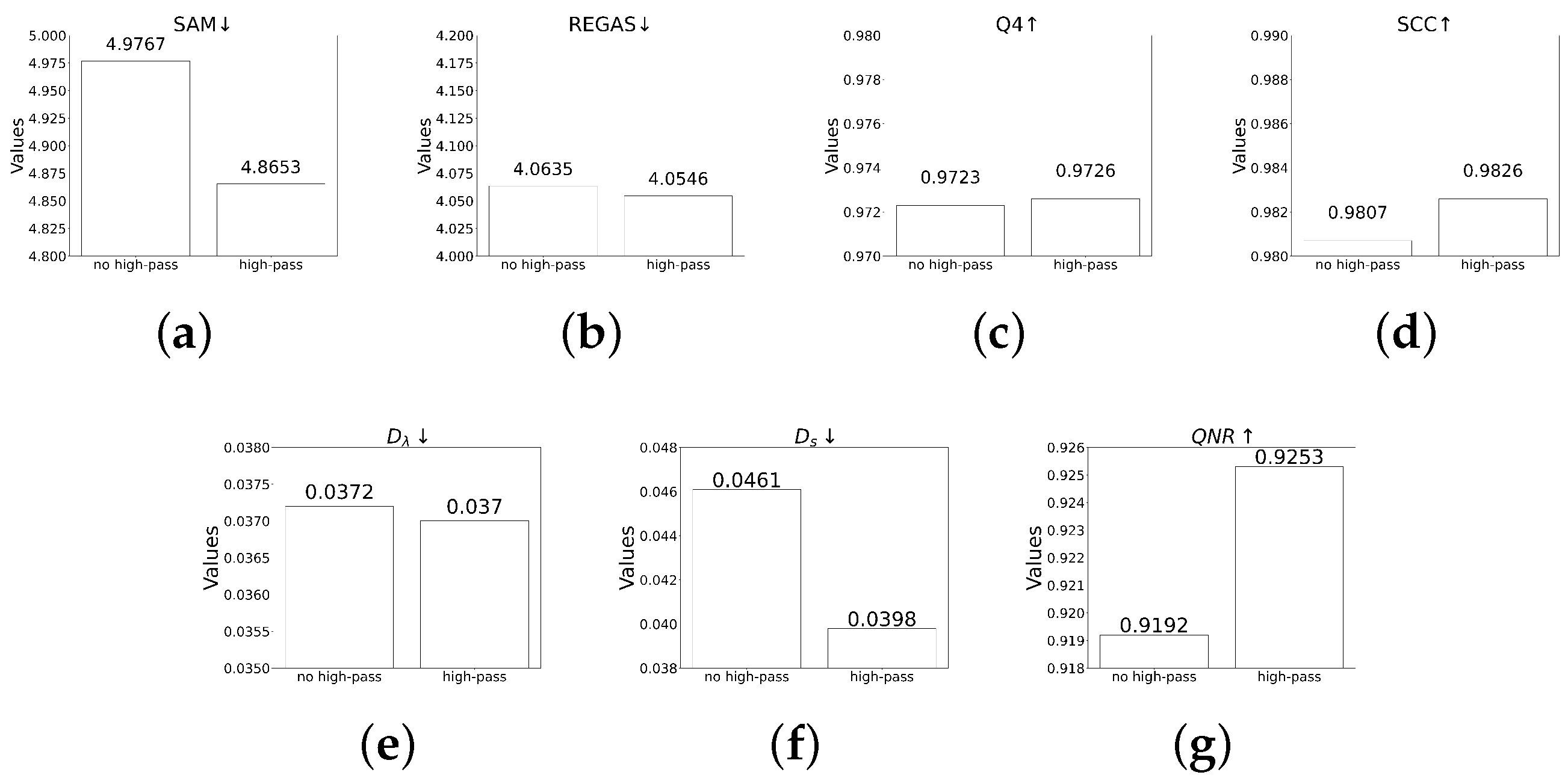
Both reduced-resolution and full-resolution metrics are evaluated on the QuickBird dataset with and without a high-pass module. As Figure 11 shows, the model with high-pass modules obtains better results in all seven metrics. It once again confirms that the high-pass module proposed by us can effectively extract spatial details, thereby improving the quality of the generated images.

5.1.2. Albation Study of Static High-Pass Preservation Module

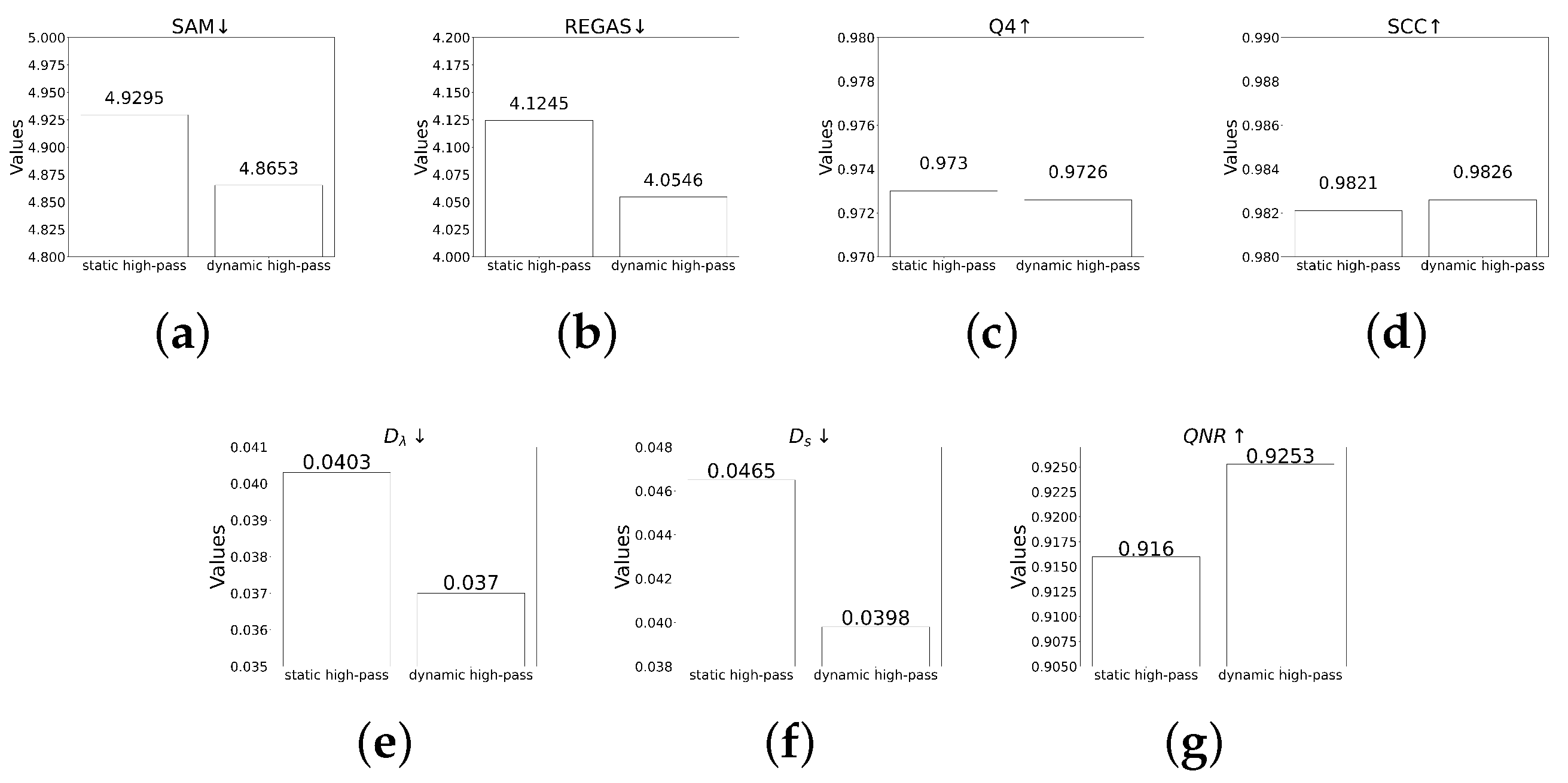
Compared to the dynamic high-pass preservation module, the static high-pass preservation module is just a simple three-layer CNN network. Both reduced-resolution and full-resolution metrics are evaluated on the QuickBird dataset with the static high-pass preservation module and the dynamic high-pass preservation module. As Figure 12 shows, the model with the dynamic high-pass module obtains better results in all seven metrics than with the static high-pass preservation module, the static high-pass preservation module even obtains worse results than those models which do not have a high-pass preservation module. This confirms that static convolution will lose some edge spatial information to some extent.

5.2. Parameter Analysis

5.2.1. Feature Dimension

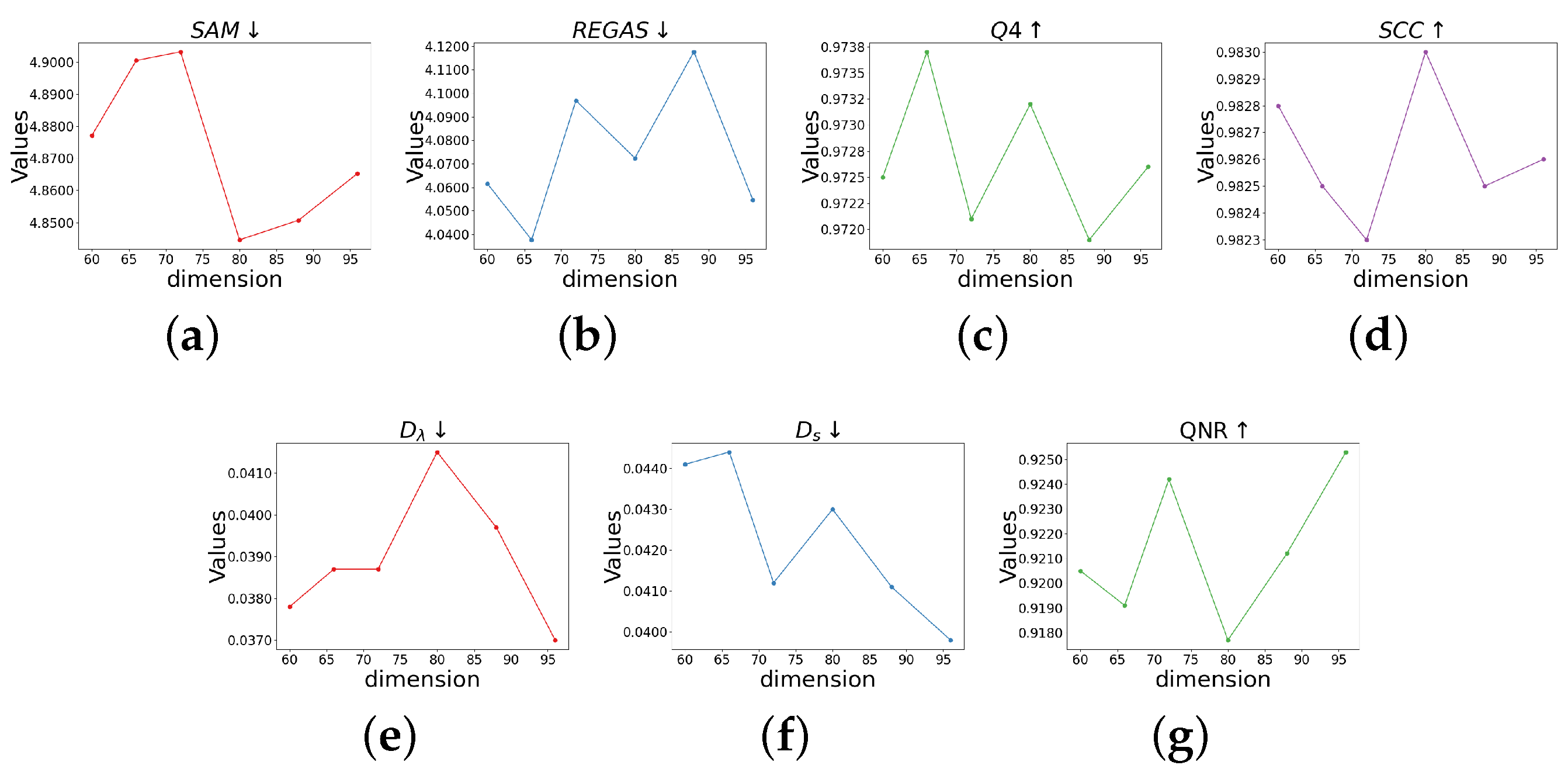
The parameter of feature dimension refers to the channel dimension of the feature map after being processed by the SFE-HP module. Experiments of different dimensions on the QuickBird dataset are conducted. Firstly, the values of metrics are not sensitive to the dimension. When the dimension changes, the values’ results do not fluctuate greatly. For the full-resolution dataset, with increasing dimension, the results become slightly better, as shown in Figure 13. For the reduced-resolution tests, as the dimension increases, the results of the experiments slightly fluctuate, and the change in feature dimension has no apparent correlation with the results of reduced-resolution metrics.

5.2.2. Number of DRLs

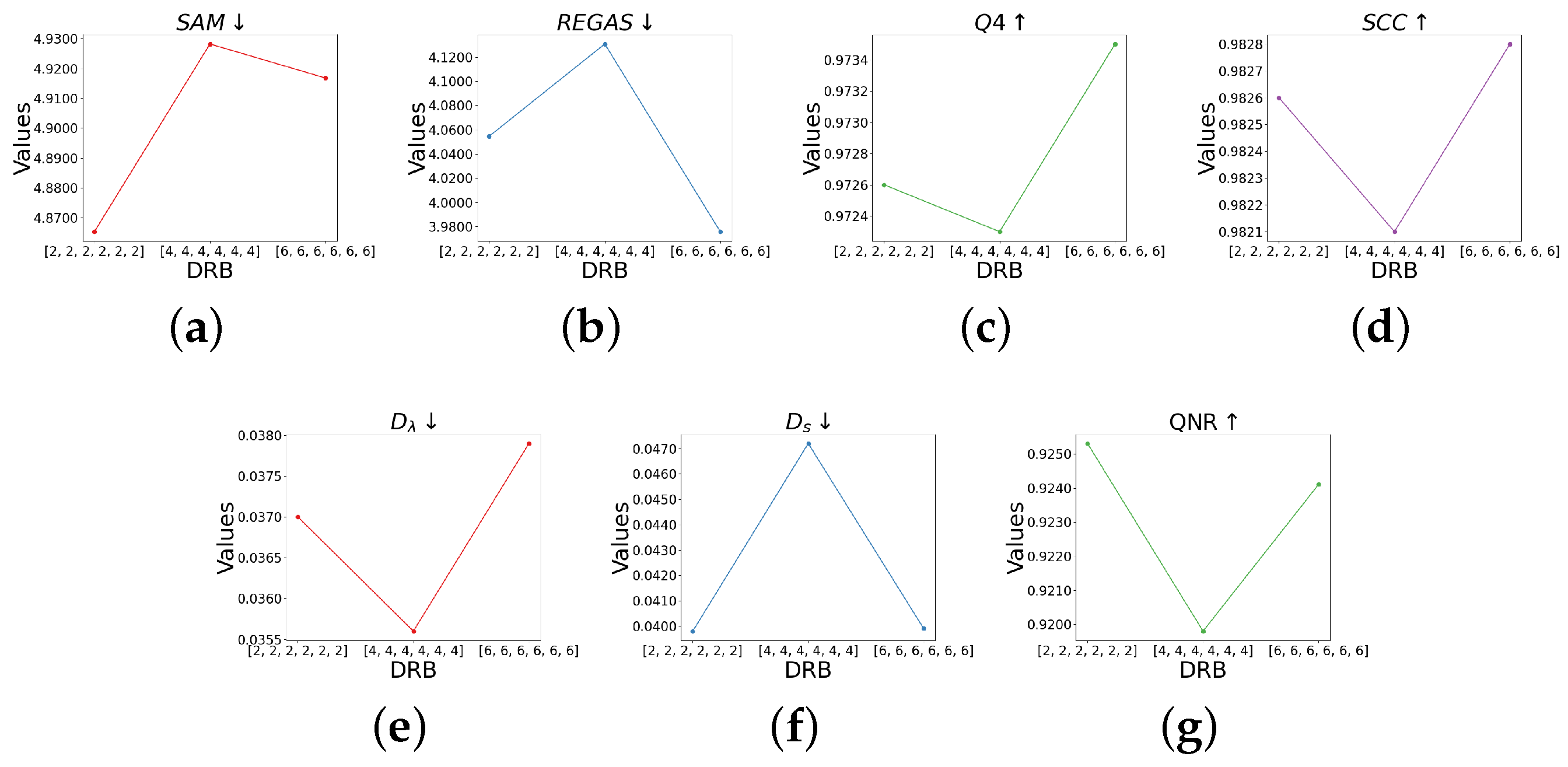
The number of DRLs in the DRB module affects the feature representation and the model complexity. As shown in Figure 14, a larger number of DRLs can enhance the representation capability of the model. As a consequence, this tends to yield larger values of metrics like Q4 and SCC on reduced-resolution tests. However, this improvement might come at the cost of reduced accuracies in full-resolution evaluation. Therefore, the acceptable number of DRLs should be carefully investigated to balance the performance of the proposed approach in the reduced- and full-resolution experiments.
The experimental results on three remote sensing datasets from different sensors have corroborated that the proposed approach is superior to other methods in the reduced- and full-resolution experiments through qualitative and quantitative analysis. The generated pansharpening results effectively reconstruct high-resolution details from PAN images while preserving the essential spectral information in the MS images. In addition, parameter analysis experiments and ablation studies were conducted. The ablation experiment particularly highlighted the efficacy of the high-pass module. The two sets of parameter analysis focused on investigating the dimension of SFE-HP and the structure of DRBs. The experimental results show that the model has strong robustness to the model’s hyperparameters. However, it is essential to acknowledge that including multihead attention mechanisms might contribute to increased model complexity, which could be considered a primary limitation of our proposed approach.

6. Conclusions

In this paper, a novel network called SwinPAN designed to address pansharpening tasks is proposed. In SwinPAN, a comprehensive transformer-based network named DRNet is proposed, building upon the Swin Transformer architecture. A dynamic high-pass preservation module is developed to enhance the high-frequency content present in shallow input features. Furthermore, it leverages content-based interactions between image content and attention weights, using a shifted-window mechanism to model long-range dependencies effectively. Comparative experiments are conducted on the QuickBird, GaoFeng2 and WorldView3 datasets. The results of these experiments demonstrate that DRNet excels in generating images enriched with fine spatial details and robust spectral information. Additionally, it surpasses previously proposed models in terms of both rendered images and evaluation metrics. In future work, semi-supervised or unsupervised learning methods for pansharpening will be investigated to reduce the labeling efforts of training samples for deep models.

Author Contributions

Data curation, W.L.; formal analysis, W.L.; methodology, W.L. and Y.H.; validation, Y.H.; visualization, Y.H. and Y.P.; writing—original draft, Y.H.; writing—review and editing, Y.H., M.H. and Y.P. All authors have read and agreed to the published version of the manuscript.

Funding

This work was supported by the National Natural Science Foundation of China (nos. 62331008, 61972060 and 62027827), the National Key Research and Development Program of China (no. 2019YFE0110800) and Special Funding for Postdoctoral Research Projects of Chongqing (no. 2022CQBSHTB3103).

Data Availability Statement

Data sharing is not applicable to this article.

Acknowledgments

The authors would like to thank all the reviewers for their valuable contributions to our work.

Conflicts of Interest

The authors declare no conflict of interest.

References

  1. Chavez, P.S., Jr.; Kwarteng, A.Y. Extracting spectral contrast in Landsat Thematic Mapper image data using selective principal component analysis. In Proceedings of the 6th Thematic Conference on Remote Sensing for Exploration Geology, Houston, TX, USA, 16–19 May 1988. [Google Scholar]
  2. Shah, V.P.; Younan, N.H.; King, R.L. An Efficient Pan-Sharpening Method via a Combined Adaptive PCA Approach and Contourlets. IEEE Trans. Geosci. Remote Sens. 2008, 46, 1323–1335. [Google Scholar] [CrossRef]
  3. Shettigara, V.K. A generalized component substitution technique for spatial enhancement of multispectral images using a higher resolution data set. Photogram. Eng. Remote Sens. 1992, 58, 561–567. [Google Scholar]
  4. Tu, T.M.; Su, S.C.; Shyu, H.C.; Huang, P.S. A new look at IHS-like image fusion methods. Inf. Fusion 2001, 2, 177–186. [Google Scholar] [CrossRef]
  5. Choi, J.; Yu, K.; Kim, Y. A New Adaptive Component-Substitution-Based Satellite Image Fusion by Using Partial Replacement. IEEE Trans. Geosci. Remote Sens. 2010, 49, 295–309. [Google Scholar] [CrossRef]
  6. Burt, P.J. The Laplacian Pyramid as a Compact Image Code. In Readings in Computer Vision; Morgan Kaufmann: Burlington, MA, USA, 1987; pp. 671–679. [Google Scholar]
  7. Mallat, S.G. A theory for multiresolution signal decomposition: The wavelet representation. IEEE Trans. Pattern Anal. Mach. Intell. 1989, 11, 674–693. [Google Scholar] [CrossRef]
  8. Antoniadis, A.; Oppenheim, G. The Stationary Wavelet Transform and some Statistical Applications. In Wavelets and Statistics; [Lecture Notes in Statistics]; Springer Science & Business Media: Berlin, Germany, 1995; Volume 103, pp. 281–299. [Google Scholar] [CrossRef]
  9. Do, M.N.; Vetterli, M. The contourlet transform: An efficient directional multiresolution image representation. IEEE Trans. Image Process. 2005, 14, 2091–2106. [Google Scholar] [CrossRef]
  10. Fang, F.; Li, F.; Shen, C.; Zhang, G. A Variational Approach for Pan-Sharpening. IEEE Trans. Image Process. A Publ. IEEE Signal Process. Soc. 2013, 22, 2822–2834. [Google Scholar] [CrossRef]
  11. Buades, A.; Coll, B.; Duran, J.; Sbert, C. Implementation of Nonlocal Pansharpening Image Fusion. Image Process. Line 2014, 4, 1–15. [Google Scholar] [CrossRef]
  12. Deng, L.J.; Feng, M.; Tai, X.C. The fusion of panchromatic and multispectral remote sensing images via tensor-based sparse modeling and hyper-Laplacian prior. Inf. Fusion 2018, 52, 76–89. [Google Scholar] [CrossRef]
  13. Devi, Y.A.S. Ranking based classification in hyperspectral images. J. Eng. Appl. Sci. 2018, 13, 1606–1612. [Google Scholar]
  14. Nayak, S.C.; Sanjeev Kumar Dash, C.; Behera, A.K.; Dehuri, S. An elitist artificial-electric-field-algorithm-based artificial neural network for financial time series forecasting. In Biologically Inspired Techniques in Many Criteria Decision Making: Proceedings of BITMDM 2021; Springer: Singapore, 2022; pp. 29–38. [Google Scholar]
  15. Merugu, S.; Tiwari, A.; Sharma, S.K. Spatial–spectral image classification with edge preserving method. J. Indian Soc. Remote Sens. 2021, 49, 703–711. [Google Scholar] [CrossRef]
  16. Zhang, X.; Yu, W.; Pun, M.O.; Shi, W. Cross-domain landslide mapping from large-scale remote sensing images using prototype-guided domain-aware progressive representation learning. ISPRS J. Photogramm. Remote Sens. 2023, 197, 1–17. [Google Scholar] [CrossRef]
  17. Zhang, X.; Zhang, B.; Yu, W.; Kang, X. Federated Deep Learning with Prototype Matching for Object Extraction From Very-High-Resolution Remote Sensing Images. IEEE Trans. Geosci. Remote Sens. 2023, 61, 1–16. [Google Scholar] [CrossRef]
  18. Dabbu, M.; Karuppusamy, L.; Pulugu, D.; Vootla, S.R.; Reddyvari, V.R. Water atom search algorithm-based deep recurrent neural network for the big data classification based on spark architecture. Int. J. Mach. Learn. Cybern. 2022, 13, 2297–2312. [Google Scholar] [CrossRef]
  19. Balamurugan, D.; Aravinth, S.; Reddy, P.C.S.; Rupani, A.; Manikandan, A. Multiview objects recognition using deep learning-based wrap-CNN with voting scheme. Neural Process. Lett. 2022, 54, 1495–1521. [Google Scholar] [CrossRef]
  20. Vitale, S. A cnn-based pansharpening method with perceptual loss. In Proceedings of the IGARSS 2019–2019 IEEE International Geoscience and Remote Sensing Symposium, Yokohama, Japan, 28 July–2 August 2019; pp. 3105–3108. [Google Scholar]
  21. Vitale, S.; Scarpa, G. A detail-preserving cross-scale learning strategy for CNN-based pansharpening. Remote Sens. 2020, 12, 348. [Google Scholar] [CrossRef]
  22. He, L.; Zhu, J.; Li, J.; Plaza, A.; Chanussot, J.; Li, B. HyperPNN: Hyperspectral pansharpening via spectrally predictive convolutional neural networks. IEEE J. Sel. Top. Appl. Earth Obs. Remote Sens. 2019, 12, 3092–3100. [Google Scholar] [CrossRef]
  23. Scarpa, G.; Vitale, S.; Cozzolino, D. Target-adaptive CNN-based pansharpening. IEEE Trans. Geosci. Remote Sens. 2018, 56, 5443–5457. [Google Scholar] [CrossRef]
  24. Jin, Z.R.; Zhang, T.J.; Jiang, T.X.; Vivone, G.; Deng, L.J. LAGConv: Local-context adaptive convolution kernels with global harmonic bias for pansharpening. In Proceedings of the AAAI Conference on Artificial Intelligence, Virtual, 22 February–1 March 2022; Volume 36, pp. 1113–1121. [Google Scholar]
  25. Deng, L.J.; Vivone, G.; Jin, C.; Chanussot, J. Detail Injection-Based Deep Convolutional Neural Networks for Pansharpening. IEEE Trans. Geosci. Remote Sens. 2020, 59, 6995–7010. [Google Scholar] [CrossRef]
  26. Yuan, Q.; Wei, Y.; Meng, X.; Shen, H.; Zhang, L. A Multiscale and Multidepth Convolutional Neural Network for Remote Sensing Imagery Pan-Sharpening. IEEE J. Sel. Top. Appl. Earth Obs. Remote Sens. 2018, 11, 978–989. [Google Scholar] [CrossRef]
  27. Yang, Y.; Tu, W.; Huang, S.; Lu, H.; Wan, W.; Gan, L. Dual-stream convolutional neural network with residual information enhancement for pansharpening. IEEE Trans. Geosci. Remote Sens. 2021, 60, 1–16. [Google Scholar] [CrossRef]
  28. Goodfellow, I.; Pouget-Abadie, J.; Mirza, M.; Xu, B.; Warde-Farley, D.; Ozair, S.; Courville, A.; Bengio, Y. Generative adversarial nets. In Proceedings of the Advances in Neural Information Processing Systems, Montreal, QC, Canada, 13 December 2014; pp. 2672–2680. [Google Scholar]
  29. Liu, Q.; Zhou, H.; Xu, Q.; Liu, X.; Wang, Y. PSGAN: A generative adversarial network for remote sensing image pan-sharpening. IEEE Trans. Geosci. Remote Sens. 2020, 59, 10227–10242. [Google Scholar] [CrossRef]
  30. Xu, Q.; Li, Y.; Nie, J.; Liu, Q.; Guo, M. UPanGAN: Unsupervised pansharpening based on the spectral and spatial loss constrained generative adversarial network. Inf. Fusion 2023, 91, 31–46. [Google Scholar] [CrossRef]
  31. Zhao, Z.; Zhan, J.; Xu, S.; Sun, K.; Huang, L.; Liu, J.; Zhang, C. FGF-GAN: A lightweight generative adversarial network for pansharpening via fast guided filter. In Proceedings of the 2021 IEEE International Conference on Multimedia and Expo (ICME), Shenzhen, China, 5–9 July 2021; pp. 1–6. [Google Scholar]
  32. Li, W.; Zhu, M.; Li, C.; Fu, H. PAN-GAN: A Generative Adversarial Network for Pansharpening. Remote Sens. 2020, 12, 1836. [Google Scholar]
  33. Xu, S.; Zhang, J.; Zhao, Z.; Sun, K.; Liu, J.; Zhang, C. Deep gradient projection networks for pan-sharpening. In Proceedings of the IEEE/CVF Conference on Computer Vision and Pattern Recognition, Nashville, TN, USA, 20–25 June 2021; pp. 1366–1375. [Google Scholar]
  34. Mifdal, J.; Tomás-Cruz, M.; Sebastianelli, A.; Coll, B.; Duran, J. Deep unfolding for hyper sharpening using a high-frequency injection module. In Proceedings of the 2023 IEEE/CVF Conference on Computer Vision and Pattern Recognition Workshops (CVPRW), Vancouver, BC, Canada, 17–24 June 2023; pp. 2106–2115. [Google Scholar]
  35. Zhou, M.; Yan, K.; Pan, J.; Ren, W.; Xie, Q.; Cao, X. Memory-augmented deep unfolding network for guided image super-resolution. Int. J. Comput. Vis. 2023, 131, 215–242. [Google Scholar] [CrossRef]
  36. Zhang, X.; Yu, W.; Pun, M.O. Multilevel deformable attention-aggregated networks for change detection in bitemporal remote sensing imagery. IEEE Trans. Geosci. Remote Sens. 2022, 60, 1–18. [Google Scholar] [CrossRef]
  37. Meng, X.; Wang, N.; Shao, F.; Li, S. Vision Transformer for Pansharpening. IEEE Trans. Geosci. Remote Sens. 2022, 60, 1–11. [Google Scholar] [CrossRef]
  38. Yin, J.; Qu, J.; Sun, L.; Huang, W.; Chen, Q. A Local and Nonlocal Feature Interaction Network for Pansharpening. Remote Sens. 2022, 14, 3743. [Google Scholar] [CrossRef]
  39. Li, S.; Guo, Q.; Li, A. Pan-Sharpening Based on CNN+ Pyramid Transformer by Using No-Reference Loss. Remote Sens. 2022, 14, 624. [Google Scholar] [CrossRef]
  40. Zhang, K.; Li, Z.; Zhang, F.; Wan, W.; Sun, J. Pan-Sharpening Based on Transformer with Redundancy Reduction. IEEE Geosci. Remote Sens. Lett. 2022, 19, 1–5. [Google Scholar] [CrossRef]
  41. Masi, G.; Cozzolino, D.; Verdoliva, L.; Scarpa, G. Pansharpening by convolutional neural networks. Remote Sens. 2016, 8, 594. [Google Scholar] [CrossRef]
  42. Dong, C.; Loy, C.C.; He, K.; Tang, X. Image Super-Resolution Using Deep Convolutional Networks. IEEE Trans. Pattern Anal. Mach. Intell. 2016, 38, 295–307. [Google Scholar] [CrossRef] [PubMed]
  43. He, L.; Rao, Y.; Li, J.; Plaza, A.; Zhu, J. Pansharpening via Detail Injection Based Convolutional Neural Networks. arXiv 2018, arXiv:1806.08898. [Google Scholar] [CrossRef]
  44. Yang, J.; Fu, X.; Hu, Y.; Huang, Y.; Paisley, J. PanNet: A Deep Network Architecture for Pan-Sharpening. In Proceedings of the 2017 IEEE International Conference on Computer Vision (ICCV), Venice, Italy, 22–29 October 2017. [Google Scholar]
  45. Dosovitskiy, A.; Beyer, L.; Kolesnikov, A.; Weissenborn, D.; Zhai, X.; Unterthiner, T.; Dehghani, M.; Minderer, M.; Heigold, G.; Gelly, S.; et al. An image is worth 16 × 16 words: Transformers for image recognition at scale. arXiv 2020, arXiv:2010.11929. [Google Scholar]
  46. Wang, N.; Meng, X.; Meng, X.; Shao, F. Convolution-Embedded Vision Transformer with Elastic Positional Encoding for Pansharpening. IEEE Trans. Geosci. Remote Sens. 2022, 60, 1–9. [Google Scholar] [CrossRef]
  47. Zhang, F.; Zhang, K.; Sun, J. Multiscale Spatial-Spectral Interaction Transformer for Pan-Sharpening. Remote Sens. 2022, 14, 1736. [Google Scholar] [CrossRef]
  48. Zhu, W.; Li, J.; An, Z.; Hua, Z. Mutiscale Hybrid Attention Transformer for Remote Sensing Image Pansharpening. IEEE Trans. Geosci. Remote Sens. 2023, 61, 1–16. [Google Scholar] [CrossRef]
  49. Liu, Z.; Lin, Y.; Cao, Y.; Hu, H.; Wei, Y.; Zhang, Z.; Lin, S.; Guo, B. Swin transformer: Hierarchical vision transformer using shifted windows. In Proceedings of the IEEE/CVF International Conference on Computer Vision, Montreal, BC, Canada, 11–17 October 2021; pp. 10012–10022. [Google Scholar]
  50. Yuhas, R.H.; Goetz, A.F.; Boardman, J.W. Discrimination among semi-arid landscape endmembers using the spectral angle mapper (SAM) algorithm. In Proceedings of the JPL, Summaries of the Third Annual JPL Airborne Geoscience Workshop. Volume 1: AVIRIS Workshop, Pasadena, CA, USA, 1–5 June 1992. [Google Scholar]
  51. Liu, X.; Liu, Q.; Wang, Y. Remote sensing image fusion based on two-stream fusion network. Inf. Fusion 2020, 55, 1–15. [Google Scholar] [CrossRef]
  52. Alparone, L.; Baronti, S.; Garzelli, A.; Nencini, F. A global quality measurement of pan-sharpened multispectral imagery. IEEE Geosci. Remote Sens. Lett. 2004, 1, 313–317. [Google Scholar] [CrossRef]
  53. Arienzo, A.; Vivone, G.; Garzelli, A.; Alparone, L.; Chanussot, J. Full-resolution quality assessment of pansharpening: Theoretical and hands-on approaches. IEEE Geosci. Remote Sens. Mag. 2022, 10, 168–201. [Google Scholar] [CrossRef]
  54. Aiazzi, B.; Baronti, S.; Selva, M. Improving Component Substitution Pansharpening Through Multivariate Regression of MS + Pan Data. IEEE Trans. Geosci. Remote Sens. 2007, 45, 3230–3239. [Google Scholar] [CrossRef]
  55. Aiazzi, B.; Alparone, L.; Baronti, S.; Garzelli, A.; Selva, M. An MTF-based spectral distortion minimizing model for pan-sharpening of very high resolution multispectral images of urban areas. In Proceedings of the 2003 2nd GRSS/ISPRS Joint Workshop on Remote Sensing and Data Fusion over Urban Areas, Berlin, Germany, 22–23 May 2003; pp. 90–94. [Google Scholar]
  56. Liu, J. Smoothing filter-based intensity modulation: A spectral preserve image fusion technique for improving spatial details. Int. J. Remote Sens. 2000, 21, 3461–3472. [Google Scholar] [CrossRef]
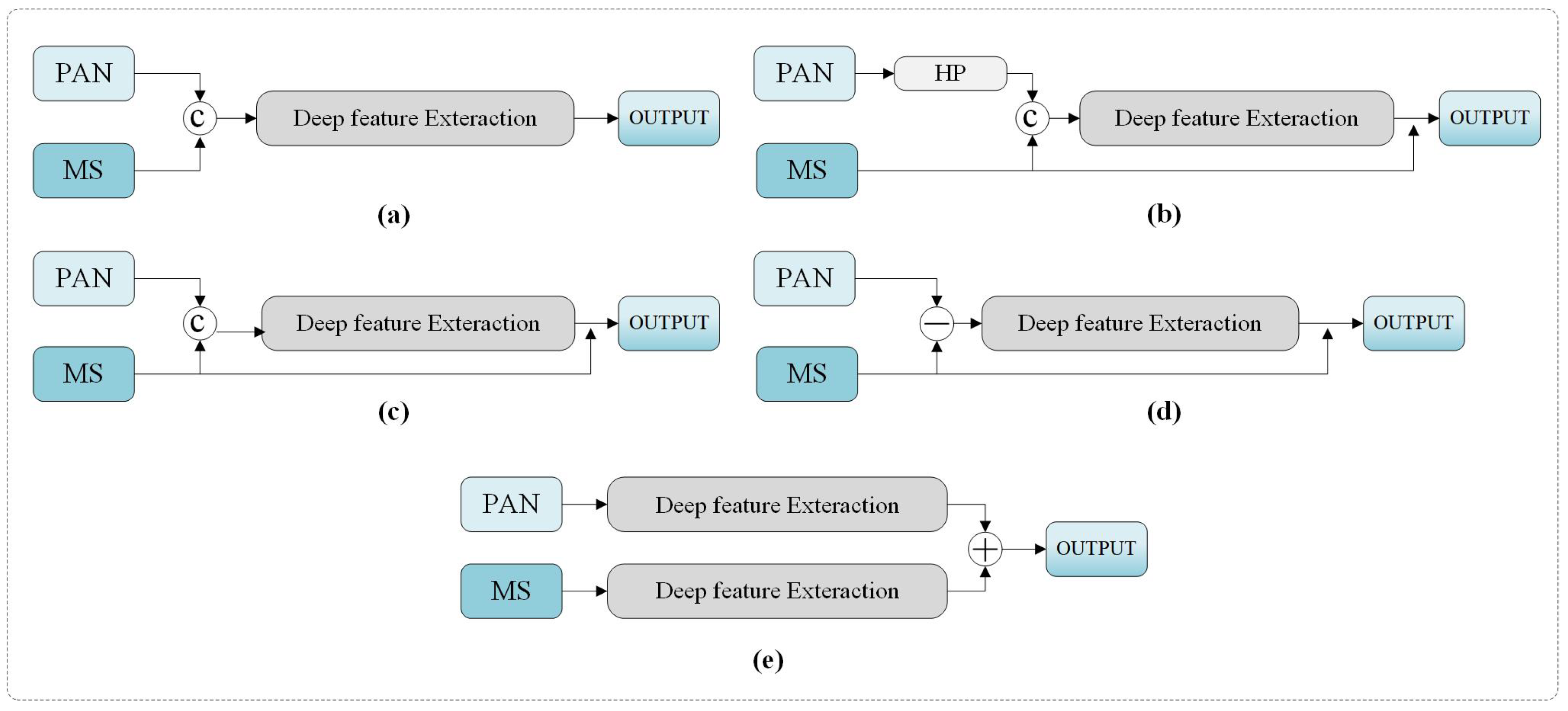
Figure 1. (ae) illustrate different frameworks of pansharpening.
Remotesensing 15 04816 g001
Figure 2. Proposed SwinPAN framework for pansharpening.
Remotesensing 15 04816 g002
Figure 3. Schematic illustration of the high-pass preservation module.
Remotesensing 15 04816 g003
Figure 4. Illustration of the self-attention module in Swin Transformer.
Remotesensing 15 04816 g004
Figure 5. Reduced-resolution results on the QuickBird imagery: (a) MS image. (b) PAN image. (c) Ground truth. (dn) Pansharpening results obtained using (d) GSA, (e) MTF-GLP-HPM, (f) SFIM, (g) DiCNN, (h) MSDCNN, (i) DRPNN, (j) FusionNet, (k) PNN, (l) PanNet, (m) HyperTransformer and (n) the proposed approach.
Remotesensing 15 04816 g005aRemotesensing 15 04816 g005b
Figure 6. Reduced-resolution results on the GaoFen2 imagery: (a) MS image. (b) PAN image. (c) Ground truth. (dn) Pansharpening results obtained using (d) GSA, (e) MTF-GLP-HPM, (f) SFIM, (g) DiCNN, (h) MSDCNN, (i) DRPNN, (j) FusionNet, (k) PNN, (l) PanNet, (m) HyperTransformer and (n) the proposed approach.
Remotesensing 15 04816 g006
Figure 7. Reduced-resolution results on the WorldView3 imagery: (a) MS image. (b) PAN image. (c) Ground truth. (dn) Pansharpening results obtained using (d) GSA, (e) MTF-GLP-HPM, (f) SFIM, (g) DiCNN, (h) MSDCNN, (i) DRPNN, (j) FusionNet, (k) PNN, (l) PanNet, (m) HyperTransformer and (n) the proposed approach.
Remotesensing 15 04816 g007
Figure 8. Full-resolution results on the QuickBird imagery: (a) MS image. (b) PAN image. (cm) Pansharpening results obtained using (c) GSA, (d) MTF-GLP-HPM, (e) SFIM, (f) DiCNN, (g) MSDCNN, (h) DRPNN, (i) FusionNet, (j) PNN, (k) PanNet, (l) HyperTransformer and (m) the proposed approach.
Remotesensing 15 04816 g008
Figure 9. Full-resolution results on the GaoFen2 imagery: (a) MS image. (b) PAN image. (cm) Pansharpening results obtained using (c) GSA, (d) MTF-GLP-HPM, (e) SFIM, (f) DiCNN, (g) MSDCNN, (h) DRPNN, (i) FusionNet, (j) PNN, (k) PanNet, (l) HyperTransformer and (m) the proposed approach.
Remotesensing 15 04816 g009
Figure 10. Full-resolution results on the WorldView3 imagery: (a) MS image. (b) PAN image. (cm) Pansharpening results obtained using (c) GSA, (d) MTF-GLP-HPM, (e) SFIM, (f) DiCNN, (g) MSDCNN, (h) DRPNN, (i) FusionNet, (j) PNN, (k) PanNet, (l) HyperTransformer and (m) the proposed approach.
Remotesensing 15 04816 g010
Figure 11. (ag) show the results of ablation study of high-pass preservation modules.
Remotesensing 15 04816 g011
Figure 12. (ag) show the results of ablation study of static high-pass preservation modules and dynamic high-pass preservation modules.
Remotesensing 15 04816 g012
Figure 13. (ag) show the results of quantitative results with different values of feature dimension.
Remotesensing 15 04816 g013
Figure 14. (ag) show the results of quantitative results with different numbers of DRBs.
Remotesensing 15 04816 g014
Table 1. Parameter settings for the proposed approach on the experimental datasets.
ParatmetersDRBDRLHeadDimensionLearning RateBatch Size
QuickBird6[2, 2, 2, 2, 2, 2]296 3 × 10 4 32
GaoFen26[2, 2, 2, 2, 2, 2]660 3 × 10 4 32
WorldView36[2, 2, 2, 2, 2, 2]260 3 × 10 4 32
Table 2. Quantative results at reduced resolution on the QuickBird dataset.
MethodsSAM↓REGAS↓Q4↑SCC↑
SFIM8.1925 ± 1.72828.8807 ± 2.12950.8495 ± 0.07880.9315 ± 0.0150
MTF-GLP-HPM8.3063 ± 1.574210.4731 ± 0.93940.8411 ±  0.01380.8796 ± 0.0194
GSA8.3497 ± 1.67289.3289 ± 2.73660.8289 ± 0.11190.9284 ± 0.0140
DiCNN5.6262 ± 0.93685.4730 ± 0.37200.9488 ± 0.01030.9712 ± 0.0054
MSDCNN4.9896 ± 0.81824.1383 ± 0.24110.9720 ± 0.00570.9814 ± 0.0038
DRPNN5.0111 ± 0.82884.1363 ± 0.24870.9719 ± 0.00570.9794 ± 0.0040
FusionNet5.1158 ± 0.84324.3962± 0.26620.9678 ± 0.00710.9797 ± 0.0039
PNN5.4115 ± 0.87054.7185 ± 0.32180.9630 ± 0.00870.9763 ± 0.0044
PanNet5.5462 ± 1.00855.4995 ± 0.80980.9487 ± 0.01860.9687 ± 0.0082
HyperTransformer4.9931 ± 0.76304.1189 ± 0.34290.9715 ± 0.00780.9813 ± 0.0075
Ours4.8653 ± 0.79094.0546 ± 0.25310.9726 ± 0.00630.9826 ± 0.0035
Table 3. Quantative results at reduced resolution on the GaoFen2 dataset.
MethodsSAM ↓REGAS ↓Q4 ↑SCC ↑
SFIM6.2068 ± 1.105012.4050 ±  2.10280.5631 ±  0.11870.9691  ± 0.0120
MTF-GLP-HPM5.1642 ±  1.033810.5863 ± 3.26070.6186  ± 0.16130.9416 ±0.0142
GSA6.4668  ± 1.001112.8536 ±2.17550.5391  ± 0.12530.9659 ± 0.0127
DICNN1.1003 ± 0.20641.1222 ± 0.21840.9840 ± 0.00810.9862 ± 0.0059
MSDCNN0.9889 ± 0.18390.9679 ± 0.17770.9886 ± 0.00630.9901 ± 0.0043
DRPNN0.9118 ± 0.16340.8185 ± 0.13770.9916 ± 0.00450.9918 ± 0.0035
FusionNet1.0143 ± 0.19591.0551 ± 0.20790.9860 ± 0.00710.9889 ± 0.0048
PNN1.0907 ± 0.21051.1116 ± 0.22590.9842 ± 0.00850.9871 ± 0.0058
PanNet1.0248 ± 0.17240.9214 ± 0.15610.9893 ± 0.00560.9898 ± 0.0043
HyperTransformer0.9538 ± 0.16480.8506 ± 0.12830.9908 ± 0.00480.9905 ± 0.0038
Ours0.7996 ± 0.14410.7790 ± 0.12710.9922 ± 0.00410.9936 ± 0.0028
Table 4. Quantative results at reduced resolution on the WorldView3 dataset.
MethodsSAM ↓REGAS ↓Q8 ↑SCC ↑
SFIM5.5385 ± 1.47375.7839 ± 1.70490.8704 ± 0.45480.9531  ± 0.0142
MTF-GLP-HPM5.7246  ± 1.50426.5285 ± 1.36220.8716 ± 0.38860.9237  ± 0.0211
GSA5.6828 ± 1.50256.6567 ± 1.80830.8732 ± 0.39730.9496 ± 0.0137
DICNN4.4534 ± 0.86433.2739 ± 0.86270.9228 ± 0.55350.9765 ± 0.0125
MSDCNN3.7875 ± 0.69422.7558 ± 0.61050.9373 ± 0.31810.9748 ± 0.0114
DRPNN3.5703 ± 0.63652.5916 ± 0.54840.8479 ± 0.45500.9778 ± 0.0119
FusionNet3.4672 ± 0.62862.5718 ± 0.59370.8516 ± 0.43760.9825 ± 0.0077
PNN3.9548 ± 0.72662.8655 ± 0.66680.8968 ± 0.48200.9750 ± 0.0109
PanNet3.7322 ± 0.66092.7974 ± 0.62700.8760 ± 0.42580.9729 ± 0.0128
HyperTransformer3.1275 ± 0.52502.6405 ± 0.51220.9210 ± 0.39700.9843 ± 0.1240
Ours2.9542 ± 0.52532.1558 ± 0.44390.9539 ± 0.47220.9890 ± 0.0046
Table 5. Quantative results at full resolution on the QuickBird dataset.
Methods D λ D s QNR↑
SFIM0.0512 ± 0.01130.1296  ± 0.09960.8243 ±  0.0974
MTF-GLP-HPM0.0506  ± 0.02340.1341 ± 0.11460.8217 ± 0.1095
GSA0.0465 ± 0.02070.2007  ± 0.10980.7614 ± 0.1033
DICNN0.0416  ± 0.03000.0910 ± 0.05140.8723 ± 0.0711
MSDCNN0.0604 ± 0.03900.0524 ± 0.01370.8903 ± 0.0391
DRPNN0.0394 ± 0.03270.0409 ± 0.02410.9219 ± 0.0513
FusionNet0.0402  ± 0.03410.0543 ± 0.04100.9088 ± 0.0676
PNN0.0399 ± 0.03420.0500 ± 0.03930.9133 ± 0.0665
PanNet0.0409 ± 0.03470.0418 ± 0.03340.9200 ± 0.0618
HyperTransformer0.0424 ± 0.03760.0412 ± 0.01950.9210 ± 0.0499
Ours0.0370 ± 0.03330.0398 ± 0.02570.9253 ± 0.0536
Table 6. Quantative results at full resolution on the GaoFen2 dataset.
Methods D λ D s QNR↑
SFIM0.0371 ± 0.01600.0647  ± 0.04600.9010  ± 0.0518
MTF-GLP-HPM0.0925  ± 0.03860.0805 ± 0.05310.8351 ± 0.0676
GSA0.0596 ± 0.02270.1027 ± 0.05420.8445 ± 0.0620
DICNN0.0179  ± 0.01450.0590 ± 0.02620.9244 ± 0.0371
MSDCNN0.0121 ± 0.01440.0387 ± 0.01980.9499 ± 0.0317
DRPNN0.0158 ± 0.01520.0319 ± 0.01680.9530 ± 0.0298
FusionNet0.0215  ± 0.01910.0546 ± 0.02620.9255 ± 0.0419
PNN0.0113 ± 0.01300.0333 ± 0.01750.9560 ± 0.0285
PanNet0.0115 ± 0.01180.0412 ± 0.01910.9486 ± 0.0285
HyperTransformer0.0174 ± 0.01700.0414 ± 0.02180.9422 ± 0.0355
Ours0.0110 ± 0.00990.0309 ± 0.01350.9585 ± 0.0210
Table 7. Quantative results at full resolution on the WorldView3 dataset.
Methods D λ D s QNR↑
SFIM0.0353 ± 0.01060.0565 ± 0.02880.9075 ± 0.0351
MTF-GLP-HPM0.0389 ± 0.02290.0523 ± 0.03320.9113  ± 0.0482
GSA0.0325 ±  0.01310.0603 ± 0.02930.9062 ± 0.0381
DICNN0.0239 ± 0.01740.0575 ± 0.03390.9202 ± 0.0410
MSDCNN0.0267 ± 0.01460.0473 ± 0.02540.9275 ± 0.0351
DRPNN0.0266 ± 0.01680.0476 ± 0.02340.9274 ± 0.0369
FusionNet0.0320 ± 0.02530.0490 ± 0.02130.9207 ± 0.0354
PNN0.0249 ± 0.01390.0451 ± 0.02200.9313 ± 0.0312
PanNet0.0277 ± 0.01420.0603 ± 0.02370.9140 ± 0.0342
HyperTransformer0.0276 ± 0.01370.0487 ± 0.02120.9347 ± 0.0312
Ours0.0216 ± 0.01050.0326 ± 0.01940.9467 ± 0.0275
Disclaimer/Publisher’s Note: The statements, opinions and data contained in all publications are solely those of the individual author(s) and contributor(s) and not of MDPI and/or the editor(s). MDPI and/or the editor(s) disclaim responsibility for any injury to people or property resulting from any ideas, methods, instructions or products referred to in the content.