Article

A Multifactor-Based Random Forest Regression Model to Reconstruct a Continuous Deformation Map in Xi’an, China

1
School of Geological Engineering and Geomatics, Chang’an University, Xi’an 710054, China
2
Key Laboratory of Western China’s Mineral Resources and Geological Engineering, Ministry of Education, Xi’an 710054, China
3
Key Laboratory of Ecological Geology and Disaster Prevention, Ministry of Natural Resources, Xi’an 710054, China
4
Department of Remote Sensing Science and Technology, Xidian University, Xi’an 710071, China
*
Author to whom correspondence should be addressed.
Remote Sens. 2023, 15(19), 4795; https://doi.org/10.3390/rs15194795
Submission received: 7 August 2023 / Revised: 27 September 2023 / Accepted: 27 September 2023 / Published: 1 October 2023
(This article belongs to the Special Issue Machine Learning and Remote Sensing for Geohazards)

Abstract

:
The synthetic aperture radar interferometry (InSAR) technique is an effective means to monitor ground deformation with high spatial resolution over large areas. However, it is still difficult to obtain the spatially continuous deformation map due to SAR decorrelation or SAR distortion, which greatly limits the usage of the InSAR deformation map, especially for spatiotemporal characterizing and mechanism inversion. Some conventional methods (e.g., spatial interpolation) rely only on the deformation measurements without considering the influence factors, leading to the inaccuracy of the deformation prediction. So, we propose a multifactor-based machine learning model, namely the K-RFR model, that combines K-means clustering and random forest regression algorithm to reconstruct a continuous deformation map, where the influence factors on ground deformation are considered, such as land use, geological engineering, and under groundwater extraction. We take the city of Xi’an, China, as the study area where SBAS-InSAR was used to obtain the ground deformation maps from 2012 to 2015. Fourteen influence factors are employed, including confined water level, change of confined water, phreatic water level, change of phreatic water, rainfall, ground fissures, stratigraphic lithology, landform, hydrogeology, engineering geology, type of land use, soil type, GDP, and DEM, where the K-means clustering method is used to reduce the influence of spatial heterogeneity. The study area is divided into three homogeneous regions and modeled independently, where the mean squared errors of region I–III are 2.9 mm, 2.3 mm, and 3.9 mm, respectively, and the mean absolute errors are 2.5 mm, 1.0 mm, and 2.8 mm, respectively. Finally, the continuous ground deformation maps of Xi’an from 2012 to 2015 are reconstructed. We compared the new method with two interpolation methods. Results show that the correlation coefficient between prediction and InSAR measurements of the new model is 0.94, whereas the ordinary Kriging method is 0.69, and the IDW method is only 0.63. This study provides an effective means to predict the continuous surface deformation over a large area.

1. Introduction

Ground deformation is a common geological phenomenon resulting from the combination of anthropogenic activities and natural functions and is characterized by long time duration and wide spatial distribution. Therefore, it is necessary to obtain the ground deformation with long time series, wide coverage, and high accuracy [1]. Traditional ground deformation monitoring methods, such as global navigation satellite systems (GNSS) and level measurements, are limited by their low spatial coverage and resolution, making them unsuitable for large-scale deformation monitoring. Interferometric synthetic aperture radar (InSAR) offers a range of substantial advantages for high spatial resolution and large-scale deformation monitoring. At present, the application of InSAR in ground subsidence monitoring is well established [2,3,4].
However, InSAR also has certain limitations when performing large-scale surface deformation monitoring. Longer spatial and temporal baselines, vegetation, and larger gradient deformations make it difficult to obtain useful information due to spatial and temporal decorrelation [5], which greatly limits the usage of the InSAR deformation map, especially for the spatiotemporal characterizing and mechanism inversion. Therefore, spatial interpolation is generally conducted to reconstruct ground deformation maps. For example, the ordinary Kriging method and the inverse distance weighted (IDW) method are used to interpolate the PS points to reconstruct the subsidence along Beijing Metro Line 6 [3,6]. However, as these methods rely on known and unknown data that have similar statistical or geometric structures, the prediction results are only mathematically significant [7]. In addition, the prediction results are easily affected by the spatial distribution of known measurements. The interpolation results are less reliable if the observations are sparse and not well distributed [8]. However, in most cases of InSAR measurements, the coherent points are not well distributed, and the influence factors and mechanisms are different over a large area, which have not been counted in the existing methods. Most of the existing ground deformation prediction models ignore the spatial heterogeneity of ground subsidence [9] caused by groundwater level changes and ground fissures distribution, which results in the low accuracy of ground deformation prediction [10].
Machine learning algorithms have been widely applied for predicting ground subsidence in the time domain [11,12,13]. Among these algorithms, the random forest model has demonstrated high accuracy in both modeling and prediction [14,15,16]. However, few studies have been reported on the reconstruction of ground subsidence [17]. Therefore, this paper proposes a machine learning approach to reconstruct (i.e., predict in the spatial domain) a large-scale continuous ground deformation map by considering the multiple influencing factors that affect ground subsidence.

2. Study Area and Datasets

2.1. Study Area

The study area, Xi’an, is located in the northern part of the Qinling Mountains, above the second and third terraces of the Weihe Alluvial Plain. The altitude of the study area is 281~796 m. The overall topography is at a low elevation from northwest to southeast, with a semi-humid continental monsoon climate, four distinct seasons, and annual precipitation ranging from 522.4 mm to 719.5 mm [18]. Xi’an has a complex geomorphology, with up to 10 loess depressions formed under tectonic action and several active fractures, of which the Weihe Fracture and the Lintong–Chang’an Fracture are the most typical [19]. Since the Eocene, thick Cenozoic strata, dominated by quaternary materials, have been deposited in the area, mainly consisting of loess, water-deposited gravels, sands, and clays, with the thickness of the loess exceeding 100 m [20]. Phreatic water is widely distributed in Xi’an, and in general, the height of the terrain influences the submerged water level, which is usually used only for farmland irrigation. Xi’an confined water aquifer is mainly divided into two layers: shallow confined water and deep confined water [21].
Due to the rapid population growth and significant increase in industrial water, surface water is difficult to meet the demand, and groundwater has become an important source of water supply. Long-term over-exploitation of groundwater is one of the causes of ground subsidence [22]. With the rapid development of Xi’an’s economy and the expansion of urban construction, the frequent construction of underground projects and high-rise buildings has become another cause of ground subsidence [23]. The combination of natural factors, such as geologic cracks and fracture zones, and anthropogenic factors, such as groundwater exploitation, has led to regional ground subsidence in some areas of Xi’an. Many researchers have conducted ground subsidence monitoring in Xi’an and obtained valuable measurements [19,22,24]. However, due to the InSAR decorrelation, there is no useful information on suburban areas and even the high-constructed areas. Therefore, we take the city of Xi’an as the study region to construct the continuous ground deformation map.

2.2. Datasets

2.2.1. SAR and DEM

We used 40 descending TerraSAR-X (TSX) images acquired from January 2012 to May 2015 to estimate the annual subsidence rate and time series in the study area using the SBAS-InSAR technique. Figure 1a shows the coverage of the SAR data. Moreover, one arc-second Shuttle Radar Topography Mission (SRTM) DEM acquired from NASA (online at https://www.nasa.gov/ (accessed on 2 March 2023)) was used to simulate and remove the topographic phases.

2.2.2. Ground Subsidence Influence Factors

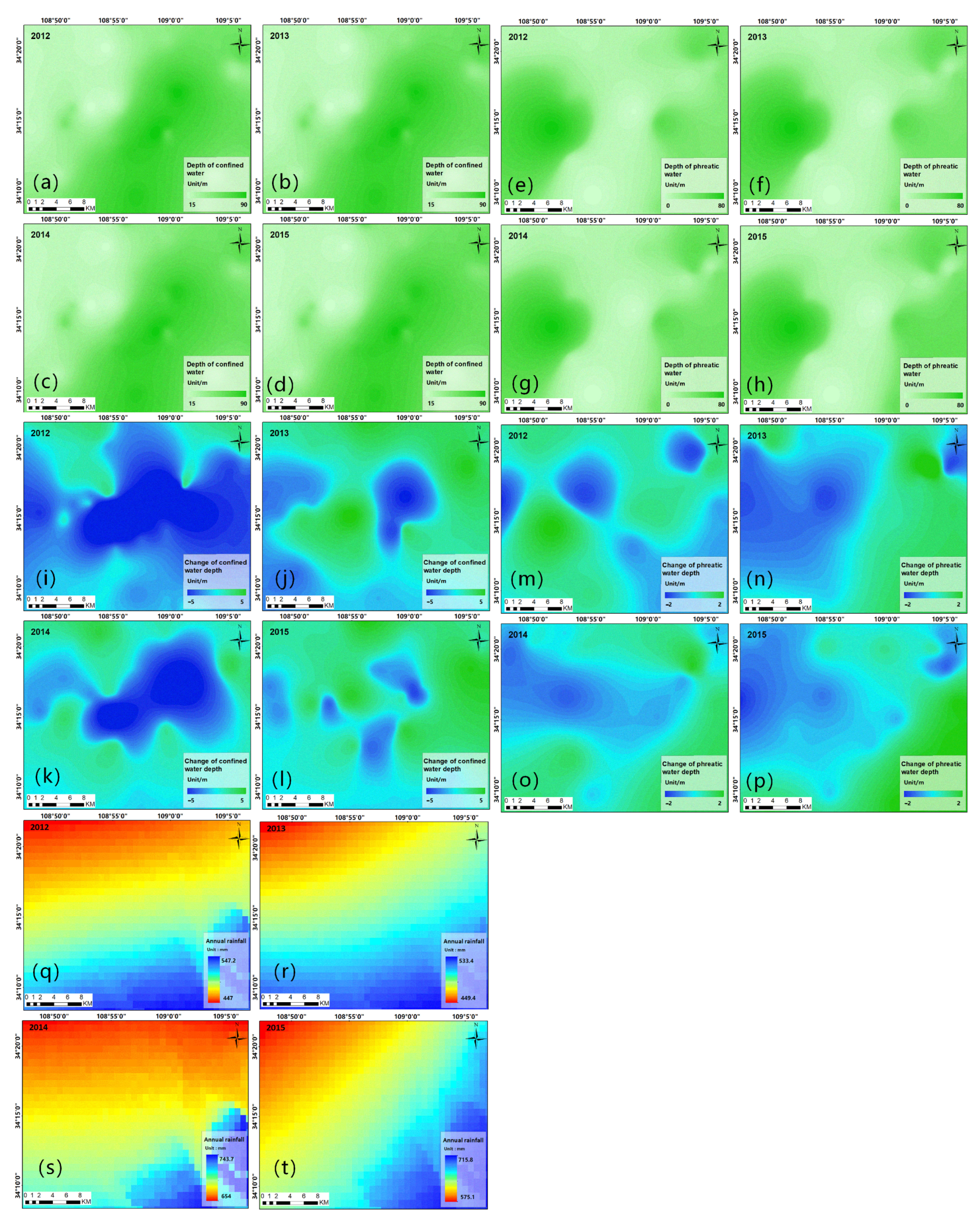
Five dynamic influence and nine static influence factors were collected. The former includes confined water level, change of confined water, phreatic water level, change of phreatic water, and rainfall. And the latter includes ground fissure, stratigraphic lithology, landform, hydrogeology, engineering geology, type of land use, soil type, GDP, and DEM. The rainfall data (online at https://disc.gsfc.nasa.gov/ (accessed on 2 March 2023)) were obtained from the National Aeronautics and Space Administration (NASA). Land use type, soil type, and GDP data (online at https://www.resdc.cn/Default.aspx (accessed on 2 March 2023)) were obtained from the Institute of Geographic Sciences and Resources, Chinese Academy of Sciences. The specifications of all factors are given in Table 1 and displayed in Appendix A and Appendix B.

3. Methodology

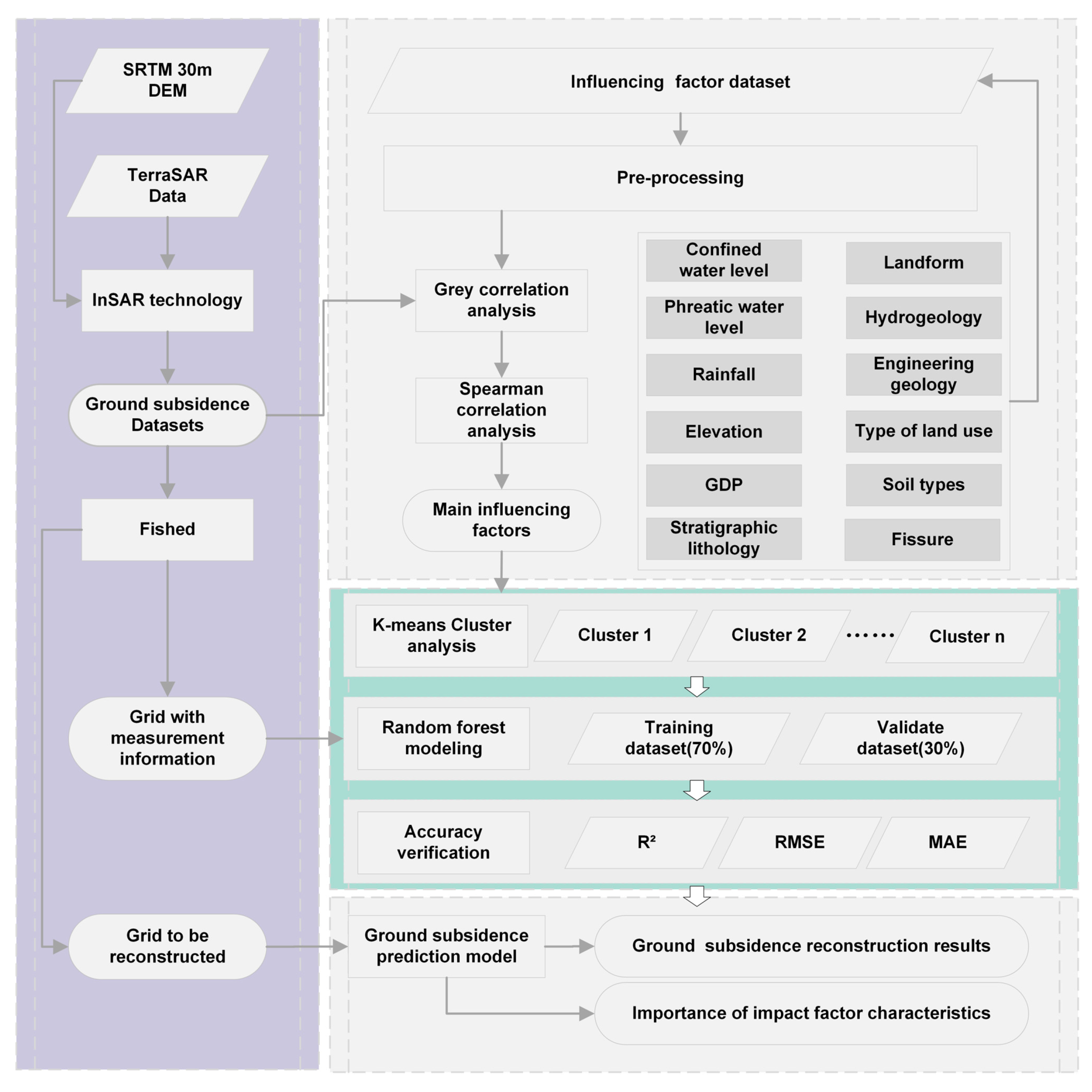
The ground deformation prediction model, namely K-RFR model, is established by coupling the K-means clustering and the random forest regression algorithm. The flowchart is shown in Figure 2, which consists of four main steps explained in the following sub-sections:

3.1. SBAS-InSAR Data Processing

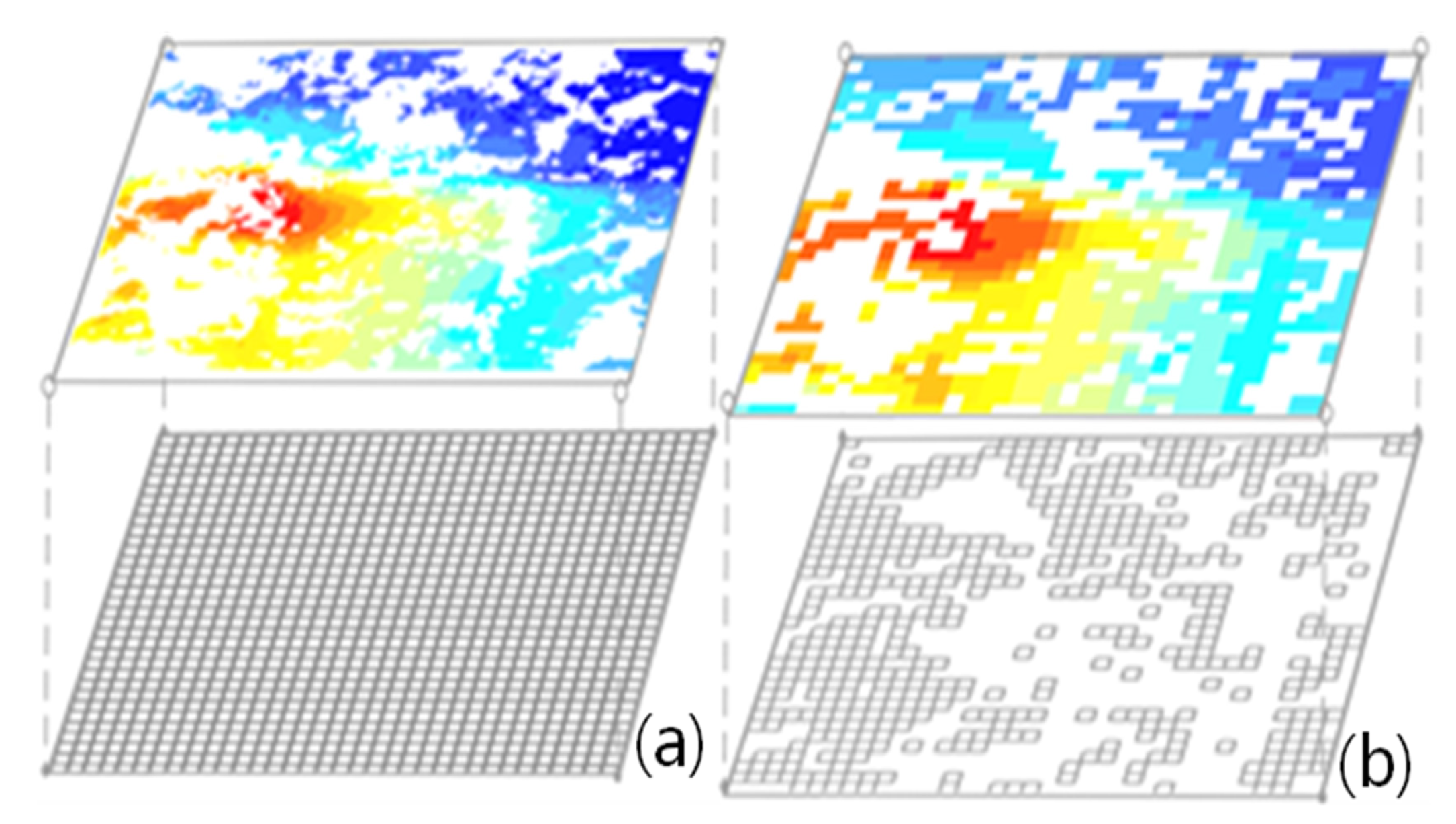
The ground subsidence rate and cumulative deformation time series are obtained by SBAS-InSAR method [25]. Then, the deformation map is gridded into small elements with resolution of 100 m × 100 m, which mainly depends on the resolution of the influence factor datasets. The average of all measurements within a grid cell is assigned as the grid measurement. And if there are no measurements within a grid cell, it should be reconstructed. The deformation map discretization process is shown in Figure 3.

3.2. Pre-Processing of Influencing Factors

As the data used in the study have different coordinate reference frames and different resolutions, before making the sample dataset, all influence data are projected uniformly into the WG84 coordinate system, and all raster datasets are resampled to the resolution of 100 × 100 m. As for the linear factors, such as ground fissures, the buffer analysis results are discretized into 100 × 100 m grid cells with buffer widths of 500 m, 1000 m, and 2000 m, respectively. The radial basis function method is used to interpolate the groundwater data to obtain the groundwater level distribution data, and the raster calculator is used to obtain the groundwater level change data.
Among the factor data, elevation, groundwater, and rainfall data belong to quantitative data, while stratigraphic lithology, geomorphologic type, hydrogeology, etc., belong to categorical data. As the coupling model of FR and the prediction model has high prediction accuracy [26], we quantify the categorical factors by frequency ratio (FR) and normalize them simultaneously with the quantitative factors [27]. FR model can accurately handle the nonlinear response relationship between deformation areas and their underlying environmental factors, which can reflect quantitative statistics on the linkage of settlement susceptibility between each attribute interval of the influencing factor. We ignore areas with subsidence rate values less than 5 mm/year, plot the overlap of predictors and subsidence locations, count the number of subsidence locations and the pixels associated with each category, and then calculate the F R values in an Excel sheet as follows.
F R = A A B B
where A is the number of ground subsidence grids in the interval for each type of environmental factor; A is the total number of ground subsidence grids in the interval; B is the number of grids in the interval where this environmental factor is located;   B is the total number of grids in the study area; and F R indicates the frequency ratio of this type of environmental factor.
To justify the suitability of the selected influence factors to build the ground deformation prediction model, the grey correlation analysis method is used to calculate the grey absolute correlation between the ground subsidence rate and the influencing factors [7,28]. The basic idea of grey correlation analysis is to determine whether the target column and the influence factor data column are closely related by determining the geometric similarity of their geometric shapes, which reflects the degree of correlation between curves. The magnitude of the correlation directly reflects the degree to which factors in the system affect the target value. In addition, the Spearman correlation coefficient is used to describe the correlation between two variables to avoid a highly linear relationship between the selected influence factors, which will affect the accuracy of prediction model construction [29,30].

3.3. Ground Deformation Prediction Model

K-mean clustering and random forest regression (K-RFR) models are coupled to build the ground deformation prediction model. First, the influence factors are clustered using the K-mean clustering algorithm to divide the study area into several homogeneous regions. Then, the samples are generated in each homogeneous region, with the influence factors as the input and ground deformation as the output, where the ratio between training set and test set is 7 to 3. Next, the random forest regression method is used to build the ground deformation prediction model. Finally, the accuracy of the model is evaluated in terms of R2, the mean absolute error (MAE), and the root mean squared error (RMSE).

3.3.1. K-Means Clustering

Ground subsidence is affected by a variety of factors, which have different spatial distributions and different degrees of influence on ground subsidence. The accuracy of the prediction model is affected by the spatial heterogeneity of the factors. The K-means clustering algorithm can reduce the influence of spatial heterogeneity when the ground deformation is predicted in a large area, which is a practical method to deal with the heterogeneity problem [31].
K-means clustering analysis is a center-based clustering algorithm in which samples are grouped into K classes in an iterative manner, and the cluster centroids are updated one by one to minimize the sum of the distances between each sample and the center or mean of the class it belongs to until the optimal clustering effect is obtained [32]. By minimizing the objective function specified in Equation (2), this algorithm assigns cluster k to data point x x j [33].
d = j = 1 k   i = 1 n   x i j c j 2
The clustering will randomly generate k initial cluster centers and assign each point to the nearest cluster center by calculating its distance from all cluster centers. After assigning all the sample points, the clustering process is completed by checking if any points need to be reassigned. If no reassignments are necessary, the clustering is finished. However, if there are points that need to be reassigned, new cluster centers are recalculated, and the point assignment process is repeated until no more points require reassignment. At that point, the cluster is considered stable, and the clustering process is completed.

3.3.2. Random Forest Regression

Random forest regression algorithm has excellent performance in ground deformation prediction [14,15]. Random forest regression (RFR) algorithm is a machine learning method for classification and regression proposed by Leo Breiman and Cutler Adele in 2001 [34]. Random forest consists of a combination of categorical regression tree (CART) algorithms, which can be divided into categorical decision trees and regression decision trees depending on the type of output variables, and the regression tree is used in this paper. Multiple regression decision trees constitute the random forest regression algorithm. The procedure of random forest regression is shown in Figure 4. The parameters that affect the accuracy of the random forest regression model mainly include the number of trees and the depth of trees. In the experiment, different input parameters are used to train and finally determine the optimal parameters of the model. Based on the concept of integrated learning, the mean value of all regression decision trees is taken as the final prediction result, which is
h ¯ ( x ) = 1 T t = 1 T   h x , θ t
where h ¯ ( x ) is the model prediction result. h x , θ t is the output based on x and θ t ; x is the independent variable; θ t is a random vector with independent identical distribution; and T is the number of regression decision trees.

3.4. Ground Deformation Prediction Model with K-RFR

The distribution of homogeneous regions and non-value sections within each homogeneous region is partitioned before constructing the prediction model. Then, the constructed K-RFR model is used to predict the ground deformation in the non-value sections. Finally, the continuous deformation region is reconstructed by combining the prediction results from different homogeneous regions. That is, the InSAR results and the predicted results are combined to generate a continuous deformation map over large area with high accuracy. In addition, the features of the random forest feature ordering are used to identify the main influencing factors of ground deformation in different clustered areas.

4. Results and Analyses

4.1. Ground Deformation Results

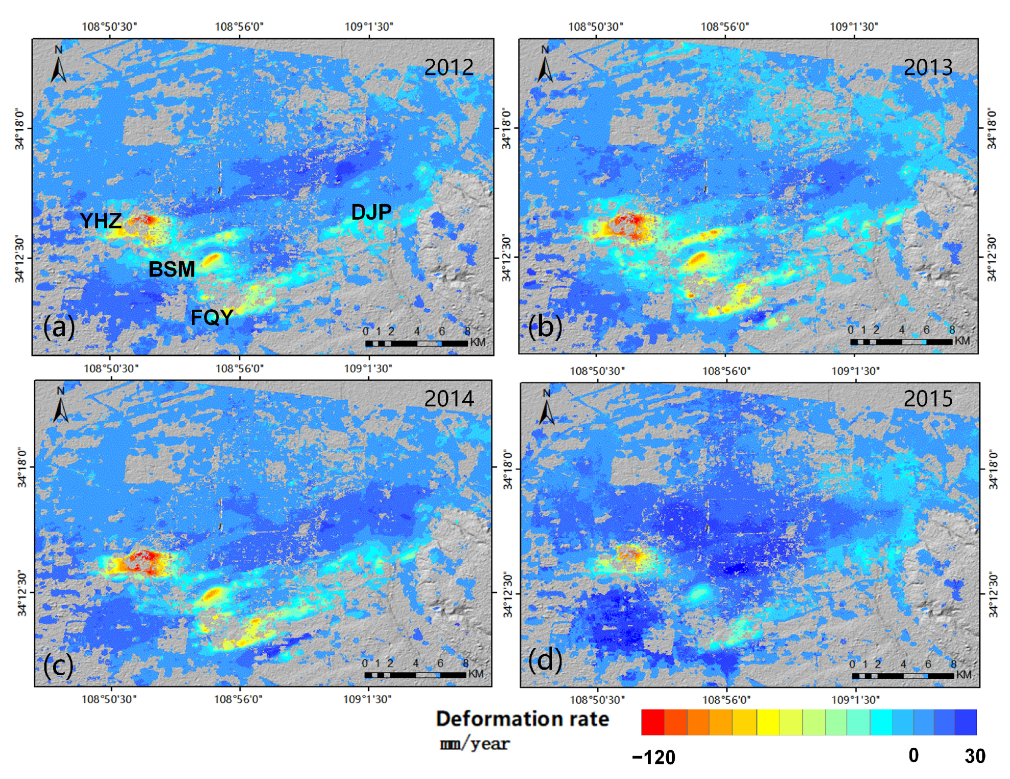
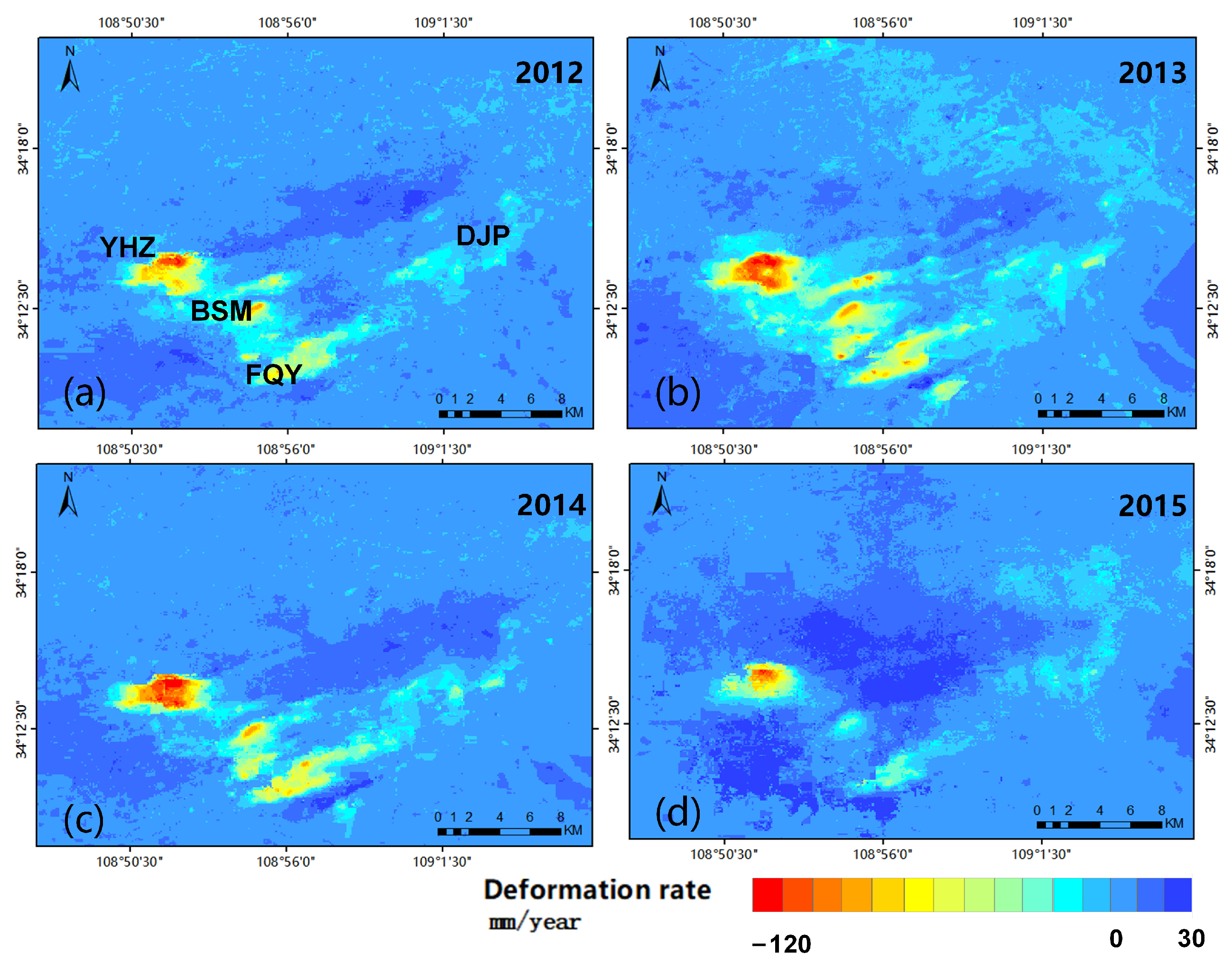
The annual average deformation rate maps of the city of Xi’an in 2012–2015 were calculated by the SBAS-InSAR technique, as shown in Figure 5. The results show that there are three subsidence areas in the city of Xi’an, which mainly occur in Yuhuazhai (YHZ), Beishanmen (BSM), and Fengqiyuan-Dengjiapo (FQY-DJP). As can be seen from Figure 5, the subsidence rate accelerated from 2012 to 2014, especially in the area of Yuhuazhai (YHZ), which reached the maximum value of 191 mm/a in 2014, and the subsidence rate slowed down from 2015, especially in the area of BSM and FQY-DJP, where the subsidence area was gradually decreasing.
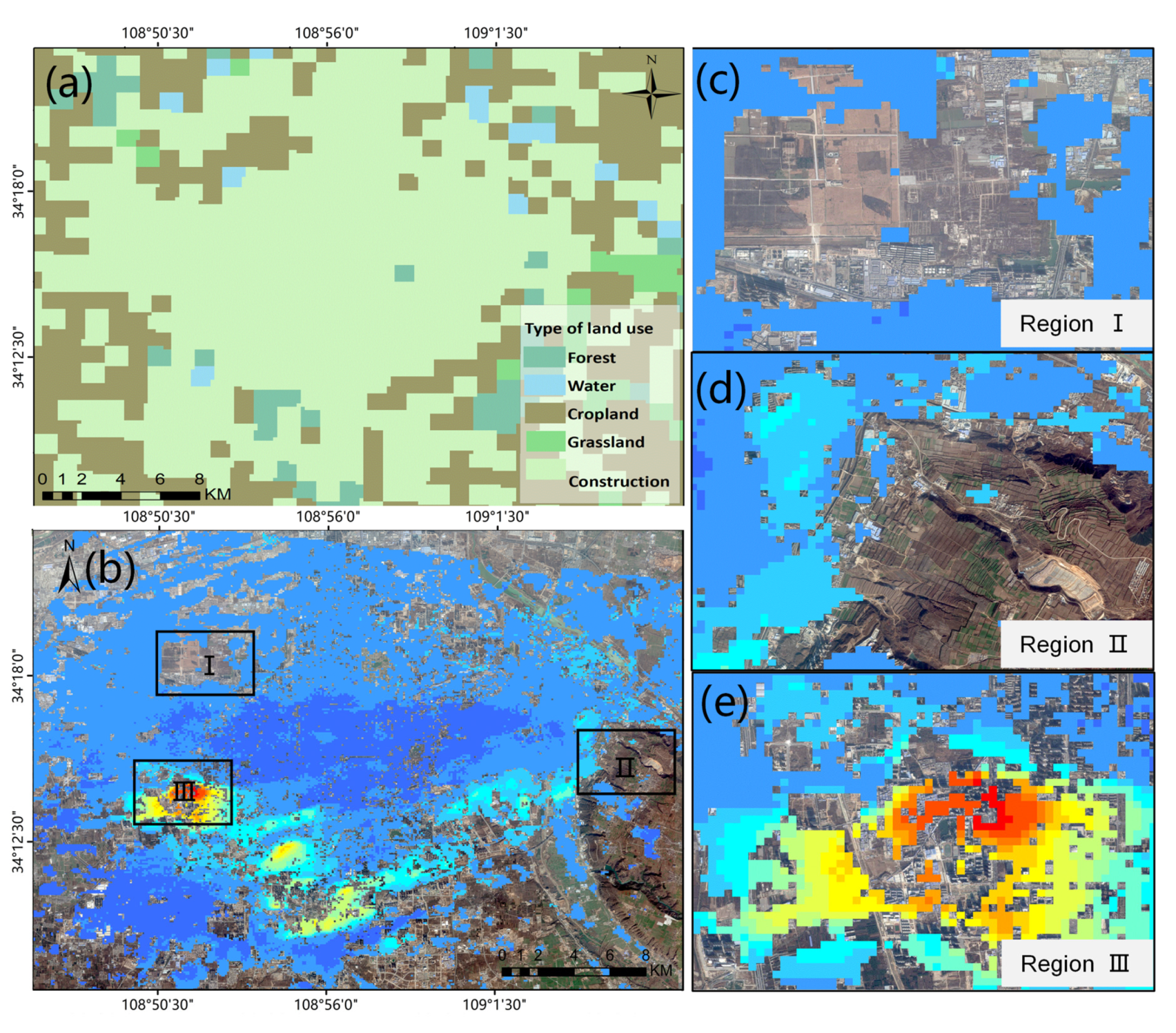
However, many measurement gaps still exist, which makes it difficult to analyze the spatiotemporal features. The ground deformation prediction model is built with K-RFR. We discretize the measurements into 100 m × 100 m grid cells; the measurement region and non-value region are gridded into 47,810 and 42,496 cells, respectively. That is, about 47% of the area needs to be reconstructed to obtain a continuous deformation map, especially in the southeastern area, where cropland, grassland, and forest in Figure 6a,d make low coherence in the SAR interferogram, and in some fast-constructed urban regions in Figure 6c,e, where surface changes degrade the coherence significantly.

4.2. Pre-Processing of Influence Factors

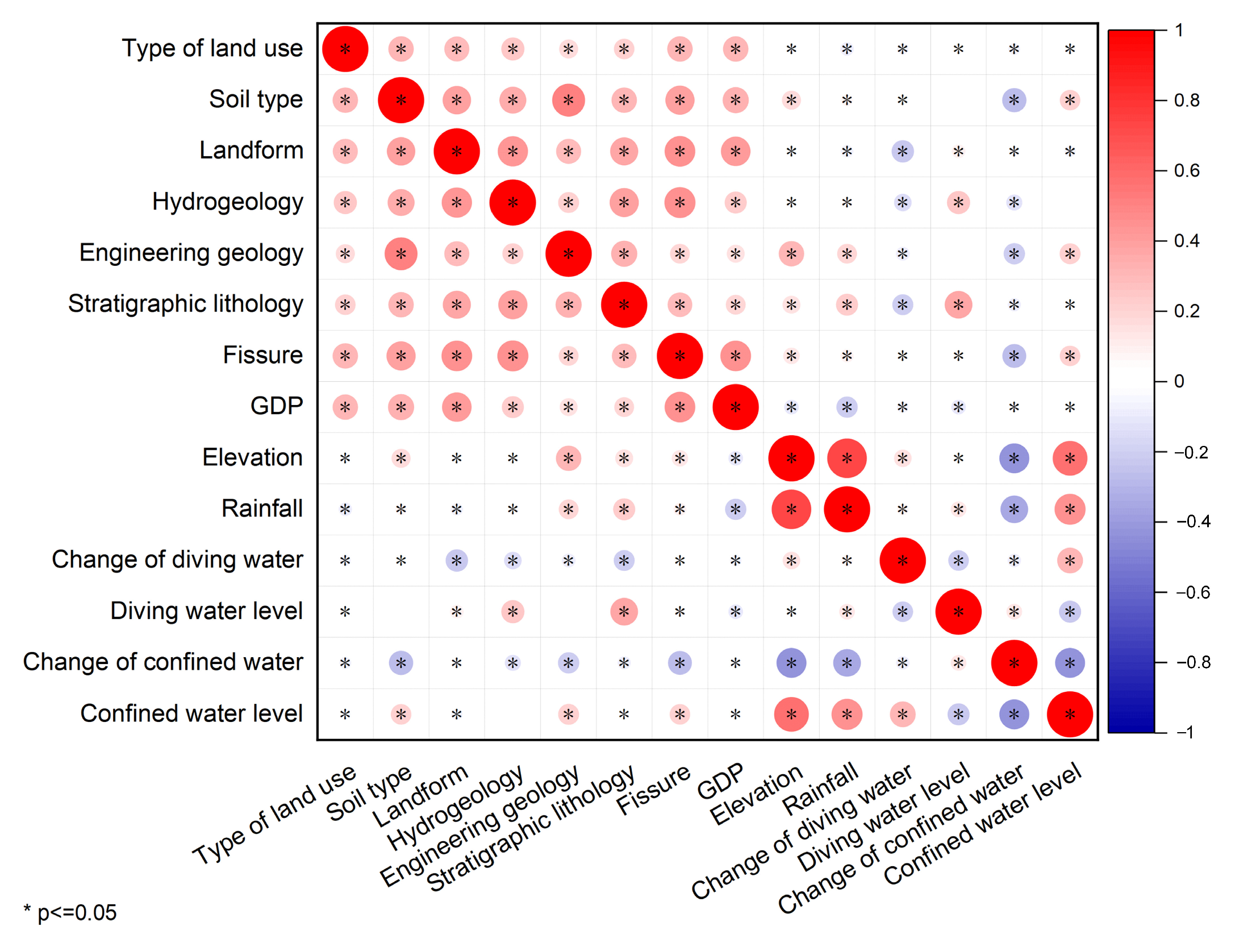
Grey correlation analysis is carried out on 14 factors, and the results are shown in Table 2, where we can see that 14 influencing factors are highly correlated with the subsidence rate, with grey correlation values greater than 0.8. The Spearman correlation coefficient between each set of two factors is less than 0.8, where the highest one between rainfall and altitude reaches 0.73, as shown in Figure 7. Therefore, 14 types of influence factors are all selected for the construction of the ground deformation prediction model.

4.3. Ground Deformation Prediction Model

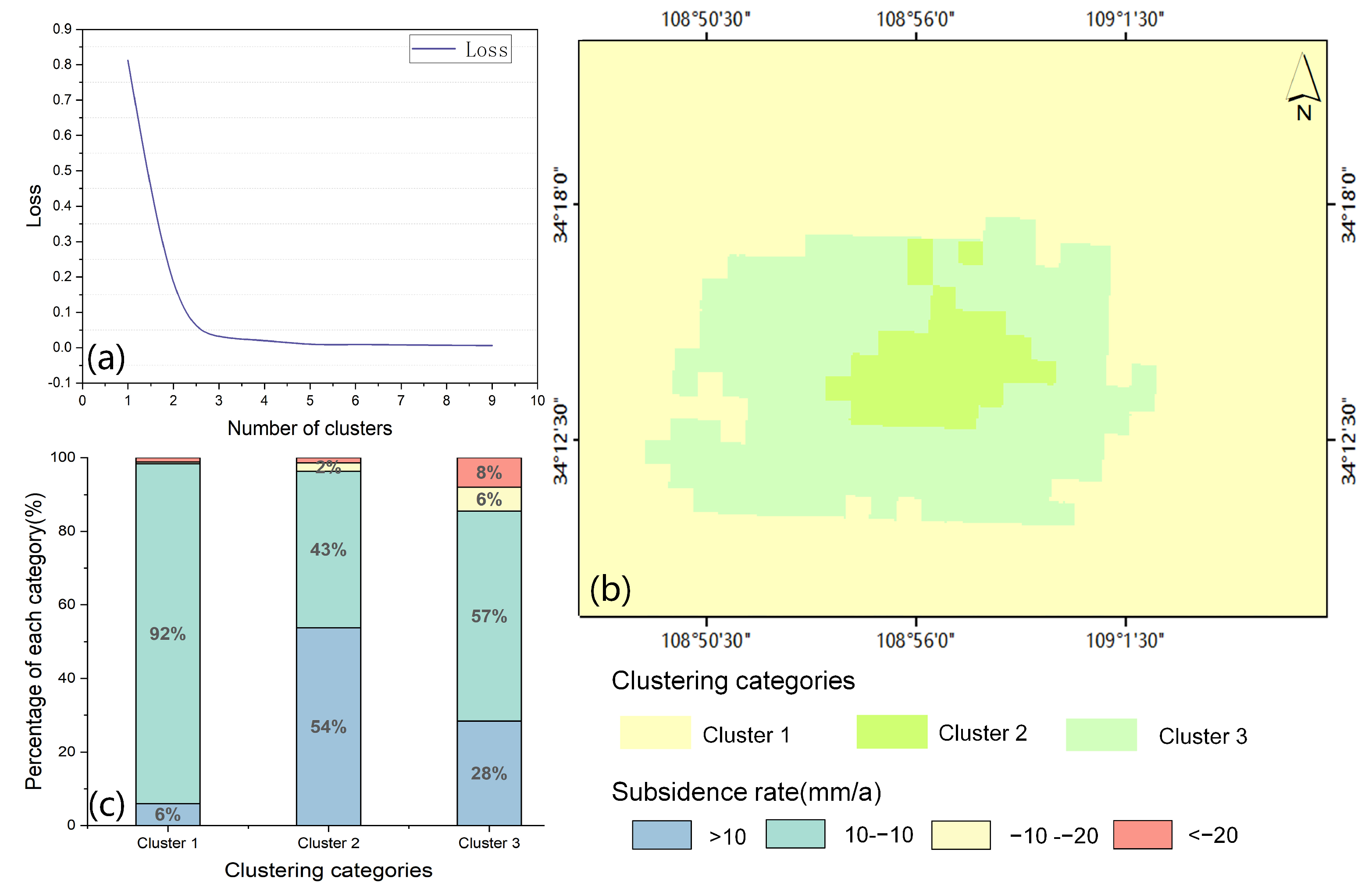
We use the “elbow method” to find the optimal number of clusters, which is 3. The loss function of the factor-averaged clustering is shown in Figure 8a. The distribution of factor clusters is shown in Figure 8b, of which Cluster 1 accounts for 74.8% of the study area, which includes most of the low subsidence rate areas, and 92% of them have an annual subsidence rate of −10 mm~10 mm. Cluster 2 only accounts for 4.5% of the study area, which includes a large number of slow upward areas, and 52% of them have a deformation rate larger than 10 mm/a. Cluster 3 is characterized by the large number of subsidence zone areas that cover about 80% of the subsidence area in the study area; in addition, the areas with the most severe subsidence, such as YHZ and BSM, are also located here. The specific distribution data of the clusters within the study area is shown in Table 3.
According to the K-means clustering results, the model training and parameter optimization of three clusters are carried out, and the parameters and evaluation indicators of the model prediction results are finally determined. The quantitative evaluation indicators of the prediction model are given in terms of R2 and OOB_SCORE (for the regression problem, that is, R2 for the out-of-bag data). In order to verify the accuracy of the model and the superiority of the coupled clustering method, 70% of the original data are randomly selected, and the ground deformation prediction model is constructed using the random forest regression model without and after sample clustering, respectively, and the remaining 30% of the data are used for comparison and verification. Table 4 shows the prediction accuracy of the different models.
The prediction accuracy of Cluster 1 (R2 = 0.89), Cluster 2 (R2 = 0.95), and Cluster 3 (R2 = 0.93) are greatly improved compared with that of pre-clustering (R2 = 0.86). The MAE is reduced from 3.4 mm to 2.5 mm, 1.0 mm, and 2.8 mm, respectively. The RMSE decreases from 4.6 mm to 2.9 mm, 2.3 mm, and 3.9 mm, respectively. The prediction accuracy of Cluster 1 improves by only 0.03 of the coefficients of determination compared with that of the pre-clustering period, which is due to the small change in ground subsidence within this cluster and the varying dominant factors for small-magnitude deformation. Due to the smaller amount of subsidence, the prediction error is also smaller.
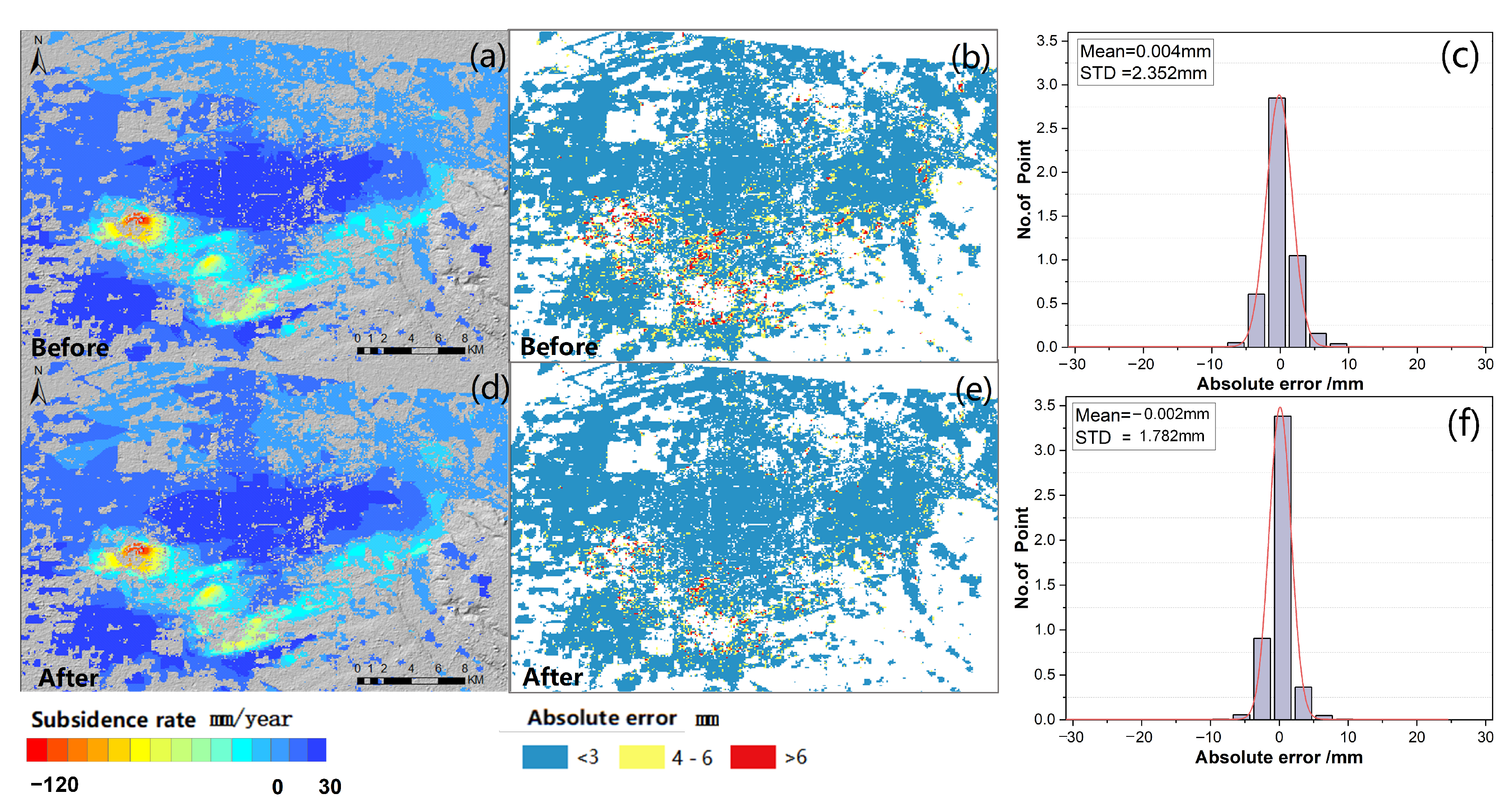
To further justify that cluster analysis improves the accuracy of the ground deformation prediction model, the absolute errors and the absolute error distribution between the prediction results of the models constructed by the two approaches and the InSAR measurements were calculated separately, as shown in Figure 9. Both clustering methods can reconstruct the ground deformation well. The absolute error value of most prediction results is less than 6 mm. Most of the larger errors are distributed in the main subsidence areas, with the error less than 10% of the subsidence rate, which can meet the requirement of prediction. Compared with the prediction results of the RFR model, the standard deviation of the K-RFR model is reduced from 2.352 mm to 1.782 mm, which verifies that the K-RFR model has higher prediction accuracy.

4.4. Application of Ground Deformation Prediction Model

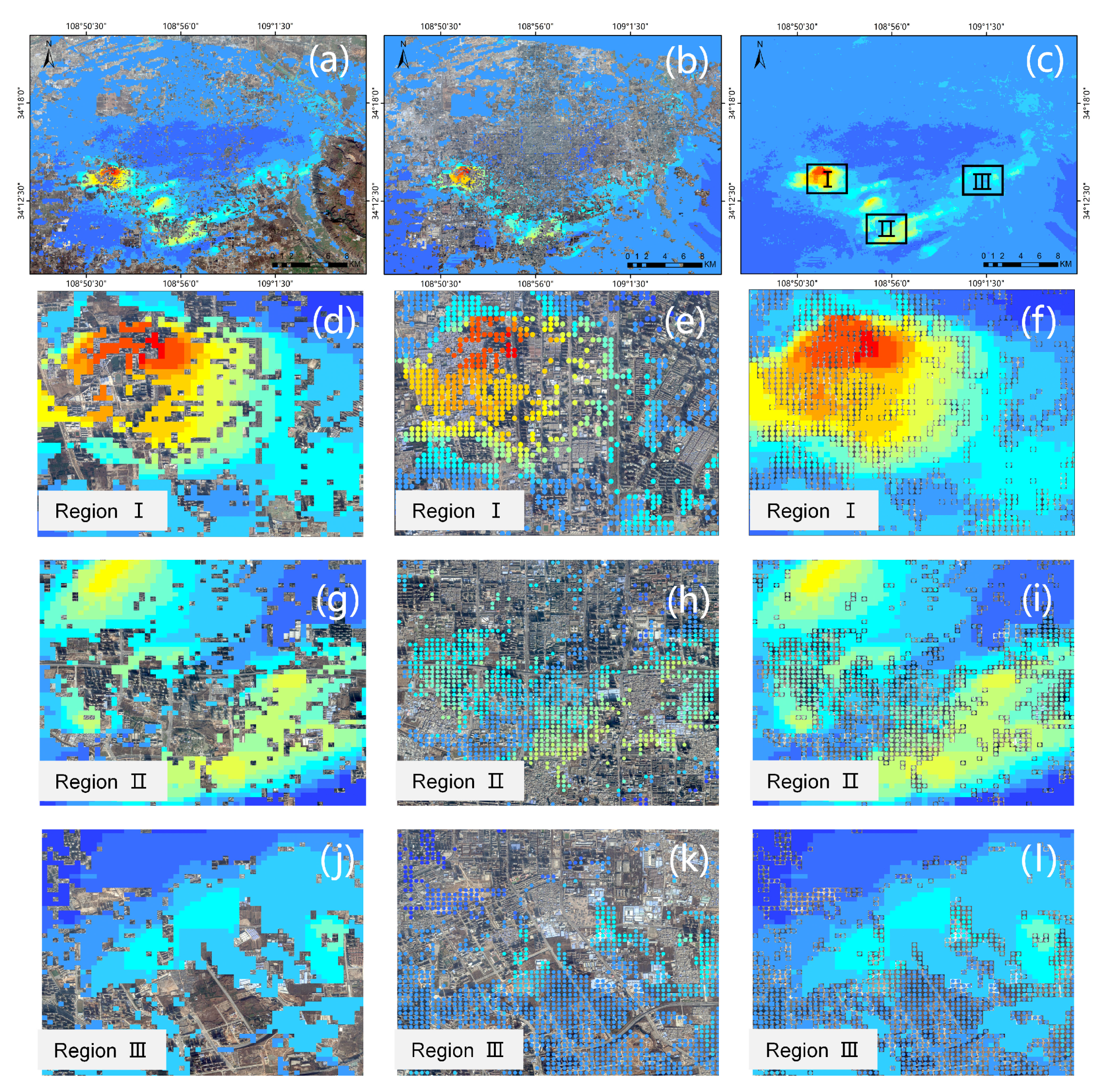
Ground deformation is predicted using the trained model and annual deformation rates from 2012 to 2015. The prediction results of the non-value areas are combined with the InSAR results on highly coherent target points to reconstruct the ground deformation of the whole study area. The reconstruction area can reach a spatial resolution of 100 m, and the combined results have good spatial continuity, as shown in Figure 10. In order to show the details of the reconstructed deformation results, three typical areas are enlarged, as shown in Figure 11. Figure 11a shows the deformation rate obtained by InSAR technology; Figure 11b shows the predicted deformation rate over the non-value region from 2012 to 2015 using the K-RFR model; Figure 11c shows the combined deformation rate results; and Figure 11d–m shows the enlarged deformation maps of three selected regions.

5. Discussion

5.1. Comparison of K-RFR Model with Conventional Methods

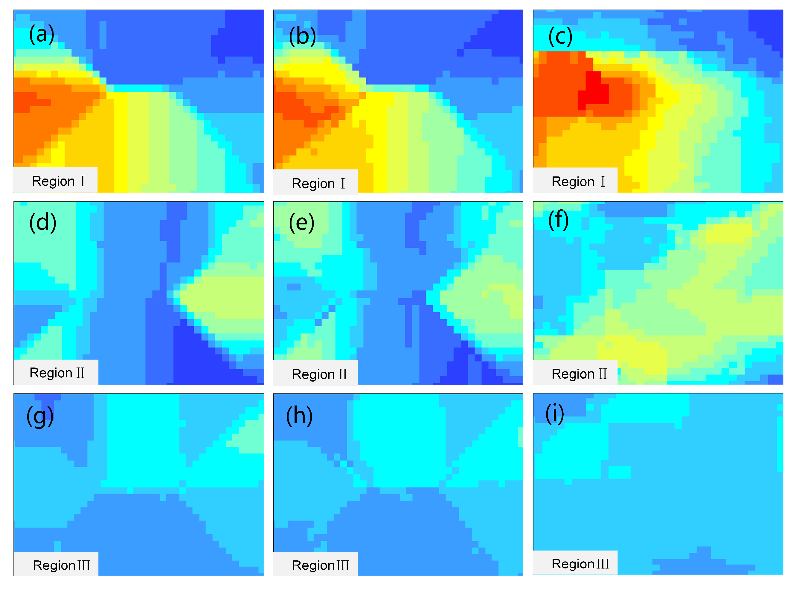
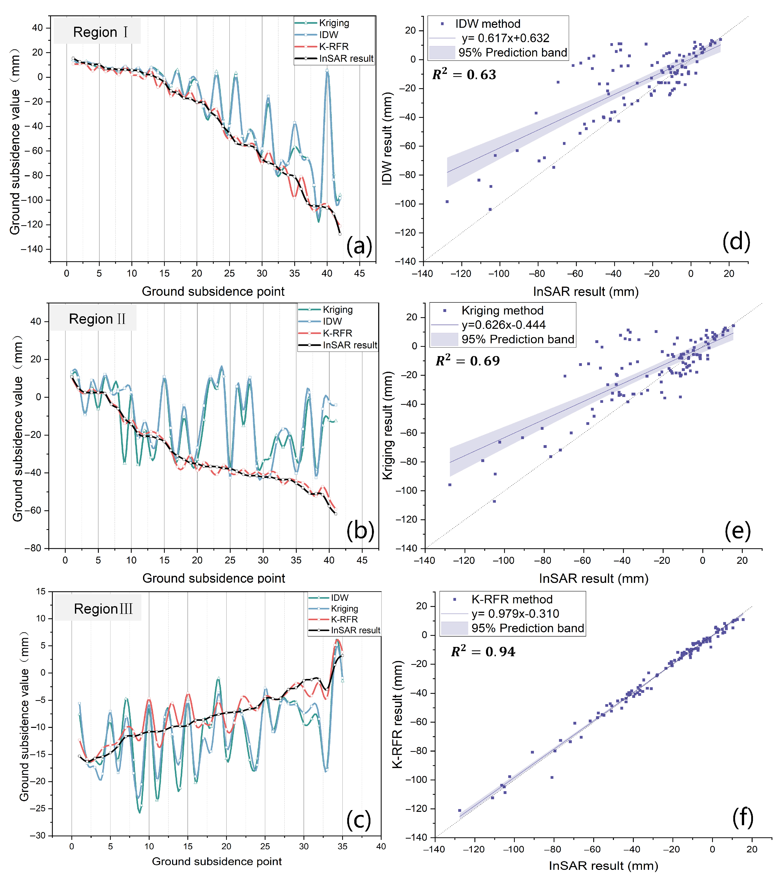
As for the K-RFR model, neither spatial high-density measurement points nor the uniform distribution of measurement points is needed. Prediction models can be constructed and predicted as long as the known measurement points are within a homogeneous region. Unlike conventional spatial interpolation methods, the K-RFR model can make full use of the existing observations and consider many influence factors, so the predicted results have better accuracy and stronger interpretability. In order to demonstrate the superiority of the proposed method in regions with sparse measurements, such as forests and cultivated land, three regions are selected for comparison. As shown in Figure 12, regions I–III, which contain a large number of measurement void regions in Figure 11c, are tested. Some known measurement points in the regions are not used for model train but as the true value for model validation. Here, we compare the K-RFR model with the commonly used Kriging and IDW interpolation methods. The results indicate that the K-RFR model can reconstruct more detailed spatial variations of ground deformation than IDW and ordinary Kriging method s. Because the variations of the influence factors are taken into account, the prediction results of the K-RFR model can reconstruct the spatial deformation pattern very well. On the contrary, the IDW and ordinary Kriging methods show discontinuous deformation results due to fewer known points near the interpolation region. Figure 13 shows the statistics of the prediction results among Kriging, IDW, and K-RFR models in regions I–III. From Figure 13a–c, we can see that the prediction from the K-RFR model has a small divergence from true values compared with the ones from IDW and ordinary Kriging models. In addition, Figure 13d–f show that the correlation between predictions from the K-RFR model and true values reaches 0.94, whereas the ones between true values and predictions from IDW and ordinary Kriging methods are 0.63 and 0.69, respectively.

5.2. Analysis of the Importance of Influence Factors

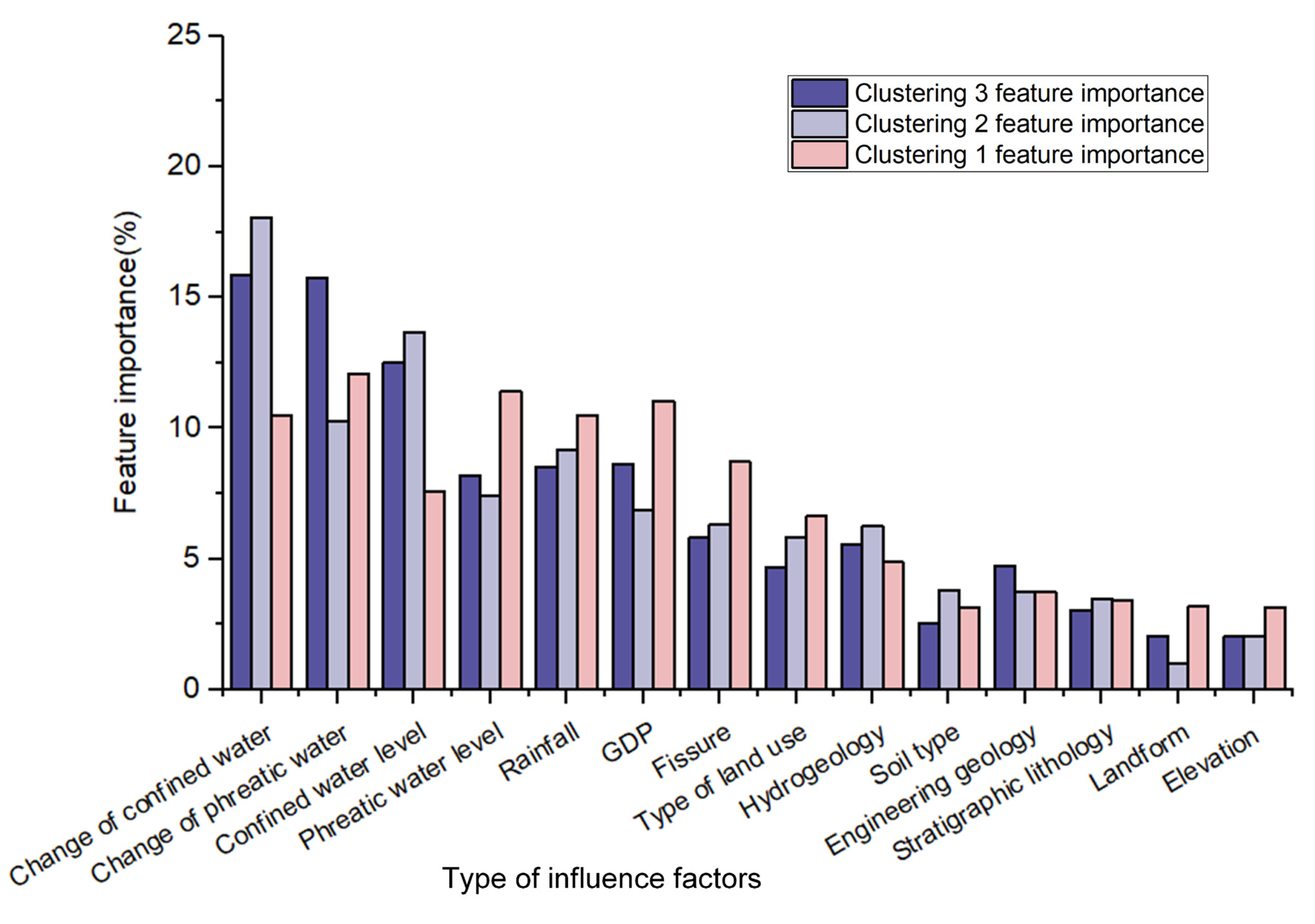
The RFR algorithm is used to explore the important influence factors of ground deformation change from 2012 to 2015, and the results are shown in Figure 14. It can be seen that the change of groundwater level and confined water level are the two most important influence factors in the study area; phreatic water level, rainfall, GDP, ground fissures, land use type, and hydrogeology are more important influence factors, and soil type, engineering geology, stratigraphic lithology, geomorphology type, and elevation are less important influence factors accounting for less than 5%. For Cluster 1, the most important influence factors are water level change, phreatic water level, rainfall, GDP, and ground fissures, and the influence of groundwater level change is relatively small. Due to the small amount of ground deformation in Cluster 1, the deformation is relatively decentralized, and the weights of influence factors are approximately the same. For Cluster 2, the main influence factors are the change of confined water level and the confined water level; in addition, the influence of factors such as phreatic water level, rainfall, and GDP is more important. Cluster 2 is composed of a large number of slowly uplifted areas, which have been governed by the Xi’an Groundwater Extraction Limit policy since 2000, especially the large amount of water injection project near the Dayan Pagoda. Cluster 3 includes the main deformation zones in Xi’an, including YHZ, BSM, and FQY-DJP. Subsidence in this area is mainly affected by the change in groundwater level, and the confined water level is an important influence factor, accounting for 43.9%. The rainfall and GDP value are also more important influence factors than any of the other factors. It can be seen that the ground deformation in Xi’an from 2012 to 2015 is mainly related to groundwater extraction, which is consistent with other research results. In order to further analyze the correlation between different factors and ground deformation, the top 70% influence factors are given and explained in detail, including groundwater levels and water level changes, rainfall, GDP, and ground fissures.

6. Conclusions

In this study, the K-RFR model is proposed to predict the continuous ground deformation map by considering multiple influence factors, where the K-means clustering method and random forest regression algorithm are coupled to improve the accuracy of the prediction model. The ground deformation results of the city of Xi’an from 2012 to 2015 are tested, where 14 influencing factors are considered. Results show that the K-RFR model can reconstruct the continuous ground deformation map with centimeter precision compared with IWD and ordinary Kriging methods.
The prediction accuracy after clustering is improved compared with that without clustering; the MAE is reduced from 3.4 mm to 2.5 mm, 1.0 mm, and 2.8 mm, respectively; and the RMSE decreases from 4.6 mm to 2.9 mm, 2.3 mm, and 3.9 mm, respectively. In addition, compared with the traditional methods, the correlation between the prediction with a new method and the true value increases from around 0.65 to 0.94.
This method is suitable for large-scale spatial deformation prediction, where multiple influencing factors make the model physically meaningful. The continuous ground deformation results attained with this method are beneficial to the spatiotemporal ground deformation characterization, mechanism explanation, and prevention decision making.

Author Contributions

Conceptualization, X.G. and G.L.; methodology, X.G.; validation, M.P. and C.Z.; data curation, X.G. and G.L.; writing—original draft preparation, X.G.; writing—review and editing, C.Z., Q.Z., G.L. and M.P.; funding acquisition, C.Z. and Q.Z. All authors have read and agreed to the published version of the manuscript.

Funding

This research is funded by the National Key R&D Program of China (No. 2022YFC3004302) and the National Natural Science Foundation of China (Grant No. 41929001). This study is also supported by the High-Performance Computing Platform of Chang’an University.

Data Availability Statement

The data that support the findings of this study are available from the author upon reasonable request.

Acknowledgments

TerraSAR-X data are provided by DLR; SRTM DEM, rainfall data are provided by the NASA Jet Propulsion Laboratory (JPL); land use, soil type, and GDP data are provided by the Institute of Geographic Sciences and Natural Resources Research, Chinese Academy of Sciences; and groundwater data are provided by the General Geological and Environmental Monitoring Station of Shaanxi Province.

Conflicts of Interest

The authors declare no conflict of interest.

Appendix A

Figure A1. Dynamic influence factors. (ad) are the confined water burial depth, (eh) are the distributions of phreatic burial depth, (il) are the distributions of changes in confined water level, (mp) are the changes in Phreatic water level, and (qt) are the distributions of average annual rainfall.
Remotesensing 15 04795 g0a1

Appendix B

Figure A2. Static influence factors. (a) is stratigraphic lithology; (b) is the type of landform; (c) is engineering geology; (d) is deep confined water hydrogeology; (e) is shallow confined water hydrogeology; (f) is phreatic hydrogeology; (g) is soil type; (h) is the total value of the GDP of the city of Xi’an in 2015; (i) is the type of land use; and (j) is the elevation map with the distribution of geosynclines.
Remotesensing 15 04795 g0a2

References

  1. Jiang, H.; Balz, T.; Cigna, F.; Tapete, D. Land subsidence in Wuhan revealed using a non-linear PSInSAR approach with long time series of COSMO-SkyMed SAR data. Remote Sens. 2021, 13, 1256. [Google Scholar] [CrossRef]
  2. Castellazzi, P.; Arroyo-Domínguez, N.; Martel, R.; Calderhead, A.I.; Normand, J.C.; Gárfias, J.; Rivera, A. Land subsidence in major cities of Central Mexico: Interpreting InSAR-derived land subsidence mapping with hydrogeological data. Int. J. Appl. Earth Obs. Geoinf. 2016, 47, 102–111. [Google Scholar] [CrossRef]
  3. Chen, B.; Gong, H.; Li, X.; Lei, K.; Zhu, L.; Gao, M.; Zhou, C. Characterization and causes of land subsidence in Beijing, China. Int. J. Remote Sens. 2017, 38, 808–826. [Google Scholar] [CrossRef]
  4. Zhang, Y.; Liu, Y.; Jin, M.; Jing, Y.; Liu, Y.; Liu, Y.; Sun, W.; Wei, J.; Chen, Y. Monitoring land subsidence in Wuhan city (China) using the SBAS-InSAR method with radarsat-2 imagery data. Sensors 2019, 19, 743. [Google Scholar] [CrossRef] [PubMed]
  5. Gao, M.; Gong, H.; Li, X.; Chen, B.; Zhou, C.; Shi, M.; Guo, L.; Chen, Z.; Ni, Z.; Duan, G. Land subsidence and ground fissures in Beijing capital international airport (bcia): Evidence from quasi-ps insar analysis. Remote Sens. 2019, 11, 1466. [Google Scholar] [CrossRef]
  6. Duan, L.; Gong, H.; Chen, B.; Zhou, C.; Lei, K.; Gao, M.; Yu, H.; Cao, Q.; Cao, J. An improved multi-sensor MTI time-series fusion method to monitor the subsidence of Beijing subway network during the Past 15 Years. Remote Sens. 2020, 12, 2125. [Google Scholar] [CrossRef]
  7. Zhou, D.; Zuo, X.; Zhao, Z. Constructing a large-scale urban land subsidence prediction method based on neural network algorithm from the perspective of multiple factors. Remote Sens. 2022, 14, 1803. [Google Scholar] [CrossRef]
  8. Shen, H.; Cheng, Q.; Zeng, C.; Yang, G.; Li, H.; Zhang, L. Missing information reconstruction of remote sensing data: A technical review. IEEE Geosci. Remote Sens. Mag. 2015, 3, 61–85. [Google Scholar] [CrossRef]
  9. Liu, Q.; Wei, J.; Wu, H.; Deng, M. HLSTM: Heterogeneous long short-term memory network for large-scale InSAR ground subsidence prediction. IEEE J. Sel. Top. Appl. Earth Obs. Remote Sens. 2021, 14, 8679–8688. [Google Scholar] [CrossRef]
  10. Deng, M.; Yang, W.; Liu, Q.; Jin, R.; Xu, F.; Zhang, Y. Heterogeneous space–time artificial neural networks for space–time series prediction. Trans. GIS 2018, 22, 183–201. [Google Scholar] [CrossRef]
  11. Hakim, W.L.; Achmad, A.R.; Lee, C.-W. Land subsidence susceptibility mapping in jakarta using functional and meta-ensemble machine learning algorithm based on time-series InSAR data. Remote Sens. 2020, 12, 3627. [Google Scholar] [CrossRef]
  12. Rahmati, O.; Golkarian, A.; Biggs, T.; Keesstra, S.; Mohammadi, F.; Daliakopoulos, I.N. Land subsidence hazard modeling: Machine learning to identify predictors and the role of human activities. J. Environ. Manag. 2019, 236, 466–480. [Google Scholar] [CrossRef]
  13. Sekkeravani, M.A.; Bazrafshan, O.; Pourghasemi, H.R.; Holisaz, A. Spatial modeling of land subsidence using machine learning models and statistical methods. Environ. Sci. Pollut. Res. 2022, 29, 28866–28883. [Google Scholar] [CrossRef] [PubMed]
  14. Ebrahimy, H.; Feizizadeh, B.; Salmani, S.; Azadi, H. A comparative study of land subsidence susceptibility mapping of Tasuj plane, Iran, using boosted regression tree, random forest and classification and regression tree methods. Environ. Earth Sci. 2020, 79, 1–12. [Google Scholar] [CrossRef]
  15. Mohammady, M.; Pourghasemi, H.R.; Amiri, M. Land subsidence susceptibility assessment using random forest machine learning algorithm. Environ. Earth Sci. 2019, 78, 503. [Google Scholar] [CrossRef]
  16. Rahmati, O.; Falah, F.; Naghibi, S.A.; Biggs, T.; Soltani, M.; Deo, R.C.; Cerdà, A.; Mohammadi, F.; Bui, D.T. Land subsidence modelling using tree-based machine learning algorithms. Sci. Total Environ. 2019, 672, 239–252. [Google Scholar] [CrossRef]
  17. Liu, Z.; Ng, A.H.M.; Wang, H.; Chen, J.; Du, Z.; Ge, L. Land subsidence modeling and assessment in the West Pearl River Delta from combined InSAR time series, land use and geological data. Int. J. Appl. Earth Obs. Geoinf. 2023, 118, 103228. [Google Scholar] [CrossRef]
  18. Qu, F.; Zhang, Q.; Lu, Z.; Zhao, C.; Yang, C.; Zhang, J. Land subsidence and ground fissures in Xi’an, China 2005–2012 revealed by multi-band InSAR time-series analysis. Remote Sens. Environ. 2014, 155, 366–376. [Google Scholar] [CrossRef]
  19. Peng, M.; Zhao, C.; Zhang, Q.; Lu, Z.; Li, Z. Research on spatiotemporal land deformation (2012–2018) over Xi’an, China, with multi-sensor SAR datasets. Remote Sens. 2019, 11, 664. [Google Scholar] [CrossRef]
  20. Peng, J.; Sun, X.H.; Wang, W.; Sun, G.C. Characteristics of land subsidence, earth fissures and related disaster chain effects with respect to urban hazards in Xi’an, China. Environ. Earth Sci. 2016, 75, 1190. [Google Scholar] [CrossRef]
  21. Li, Y. Study on the Mechanism of Ground Crack Activity and Effective Influence Distance in Xi’an. Master’s Thesis, Chang’an University, Xi’an, China, 2020. [Google Scholar]
  22. Li, G.; Zhao, C.; Wang, B.; Peng, M.; Bai, L. Evolution of spatiotemporal ground deformation over 30 years in Xi’an, China, with multi-sensor SAR interferometry. J. Hydrol. 2023, 616, 128764. [Google Scholar] [CrossRef]
  23. Solari, L.; Ciampalini, A.; Raspini, F.; Bianchini, S.; Moretti, S. PSInSAR Analysis in the Pisa Urban Area (Italy): A Case Study of Subsidence Related to Stratigraphical Factors and Urbanization. Remote Sens. 2016, 8, 120. [Google Scholar] [CrossRef]
  24. Zhao, C.; Zhang, Q.; Ding, X.L.; Lu, Z.; Yang, C.S.; Qi, X.M. Monitoring of land subsidence and ground fissures in Xian, China 2005–2006: Mapped by SAR interferometry. Environ. Geol. 2009, 58, 1533–1540. [Google Scholar] [CrossRef]
  25. Berardino, P.; Fornaro, G.; Lanari, R.; Sansosti, E. A new algorithm for surface deformation monitoring based on small baseline differential SAR interferograms. IEEE Trans. Geosci. Remote Sens. 2002, 40, 2375–2383. [Google Scholar] [CrossRef]
  26. Li, W.; Hai, X.; Hang, F.; Wu, X.; Yin, K.; Chang, Z. Uncertainty in Landslide Vulnerability Modeling with Different Environmental Factor Linkages and Predictive Models. Earth Sci. Res. J. 2021, 46, 3777–3795. [Google Scholar]
  27. Pradhan, B.; Lee, S. Landslide susceptibility assessment and factor effect analysis: Backpropagation artificial neural networks and their comparison with frequency ratio and bivariate logistic regression modelling. Environ. Model. Softw. 2010, 25, 747–759. [Google Scholar] [CrossRef]
  28. Shi, Y.; Shi, D.; Cao, X. Impacting factors and temporal and spatial differentiation of land subsidence in Shanghai. Sustainability 2018, 10, 3146. [Google Scholar] [CrossRef]
  29. Chen, B.; Gong, H.; Li, X.; Lei, K.; Ke, Y.; Duan, G.; Zhou, C. Spatial correlation between land subsidence and urbanization in Beijing, China. Nat. Hazards 2015, 75, 2637–2652. [Google Scholar] [CrossRef]
  30. Li, F.; Gong, H.; Chen, B.; Zhou, C.; Guo, L. Analysis of the contribution rate of the influencing factors to land subsidence in the Eastern Beijing plain, China based on extremely randomized trees (ERT) method. Remote Sens. 2020, 12, 2963. [Google Scholar] [CrossRef]
  31. Taravatrooy, N.; Nikoo, M.R.; Sadegh, M.; Parvinnia, M. A hybrid clustering-fusion methodology for land subsidence estimation. Nat. Hazards 2018, 94, 905–926. [Google Scholar] [CrossRef]
  32. Xue, L.; Wang, J. Improved k-means algorithm based on optimizing initial cluster centers and its application. Int. J. Adv. Netw. Monit. Control. 2017, 2, 9–16. [Google Scholar]
  33. James, M. Some methods for classification and analysis of multivariate observations. In Proceedings of the Fifth Berkeley Symposium on Mathematical Statistics and Probability; University of California Press; Oakland, CA, USA, 1967. [Google Scholar]
  34. Breiman, L. Random Forests. Mach. Learn. 2001, 45, 5–32. [Google Scholar] [CrossRef]
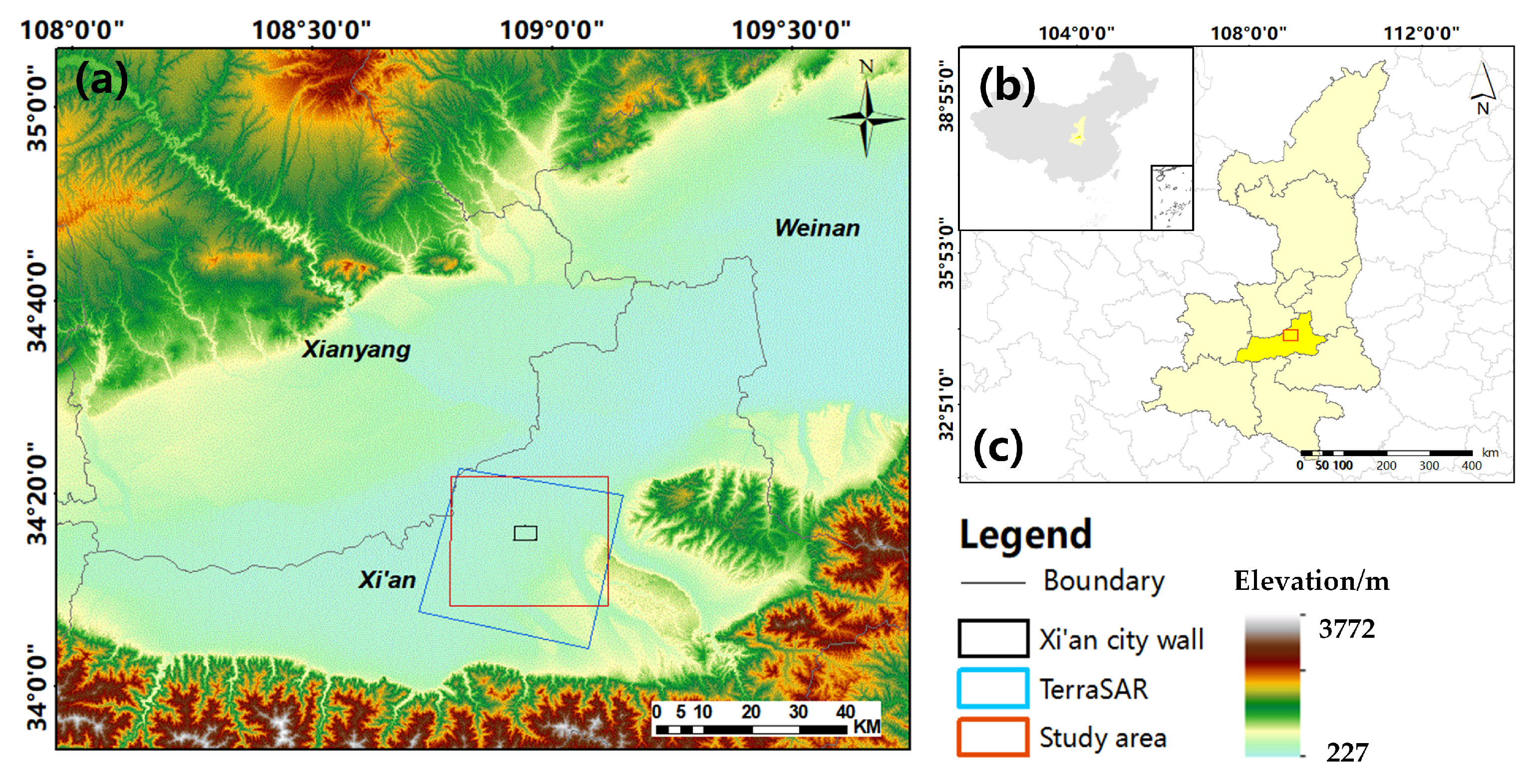
Figure 1. Overview of the study area. (a) Location of the study area and SRTM DEM with TerraSAR data superimposed. (b) Location of the study area in China. (c) Location of Shaanxi Province within China.
Remotesensing 15 04795 g001
Figure 2. Flowchart of continuous ground subsidence reconstruction in large area.
Remotesensing 15 04795 g002
Figure 3. The deformation map discretization process. (a) before discretization, including the raster data and grid cells used for discretization; (b) after discretization, including the grid regions with and without measurements after discretization.
Remotesensing 15 04795 g003
Figure 4. The procedure of random forest regression.
Remotesensing 15 04795 g004
Figure 5. Annual average deformation rate obtained by InSAR technology from 2012 to 2015. (ad) show the average annual deformation rate maps for 2012, 2013, 2014, and 2015, respectively.
Remotesensing 15 04795 g005
Figure 6. Land use classification map and optical image overlaid with InSAR annual deformation map of Xi’an. (a) show type of land use of Xi’an. (b)show map of average deformation rates from 2012 to 2015. (ce) show detailed maps of regions I–III in (b).
Remotesensing 15 04795 g006
Figure 7. Correlation results using the influence factor of the Spearman correlation coefficient.
Remotesensing 15 04795 g007
Figure 8. The clustering results and the statistics of the subsidence distribution within each cluster. (a) the K-means clustering loss function. (b) the distribution of clustering results. (c) the percentage of ground deformation in three clusters.
Remotesensing 15 04795 g008
Figure 9. Clustering comparisons. (a,d) are the predicted results of deformation before and after clustering, respectively; (b,c) are the absolute error and error distribution before clustering; (e,f) are the absolute error and error distribution after clustering.
Remotesensing 15 04795 g009
Figure 10. Ground deformation rate maps from 2012 to 2015 after reconstruction with K-RFR model. (ad) show the ground annual deformation rate maps for 2012, 2013, 2014, and 2015 after reconstruction, respectively.
Remotesensing 15 04795 g010
Figure 11. InSAR deformation maps, prediction maps, and reconstruction maps. (a) InSAR deformation map of the high coherence target points; (b) predicted deformation map; (c) reconstructed deformation map by combining (a,b); (d,g,j) enlarged InSAR deformation maps over regions I–III, respectively; (e,h,k) enlarged predicted deformation maps of regions I–III, respectively; (f,i,l) enlarged reconstructed deformation maps of regions I–III, respectively.
Remotesensing 15 04795 g011
Figure 12. Comparison of among K-RFR prediction and Kriging and IDW interpolations in regions I–III. (a,d,g) the Kriging interpolation results; (b,e,h) the IDW interpolation results; and (c,f,i) the prediction results of K-RFR model.
Remotesensing 15 04795 g012
Figure 13. Statistics of the prediction results of Kriging, IDW, and K-RFR models in regions I–III. (ac) the true values and the predicted values with three methods in regions I–III. (df) the correlation between true values and prediction values from IDW, ordinary Kriging, and K-RFR models, respectively.
Remotesensing 15 04795 g013
Figure 14. Percentage importance of the influence factors of ground deformation under different clusters obtained by random forest model.
Remotesensing 15 04795 g014
Table 1. The resources and specifications of influence factors.
Influence FactorsFormatResolutionData SourcesDuration
Ground subsidenceRaster3 m × 3 mInSAR results2012–2015
Ground fissureVectorMap data2012
Stratigraphic lithologyRaster100 m × 100 mMap data2012
Engineering geologyRaster100 m × 100 mMap data2012
LandformRaster100 m × 100 mMap data2012
DEMRaster30 × 30 mNASA2015
HydrogeologyDeep confined waterRaster100 m × 100 mMap data2012
Shallow confined water100 m × 100 m
Phreatic water100 m × 100 m
GroundwaterConfined water levelVectorGeological Environment Monitoring Station2012–2015
Phreatic water level
RainfallRaster1 km × 1 kmGoddard Earth Sciences Data and Information Services Center2012–2015
Land useRaster1 km × 1 kmInstitute of Geographic Sciences and Natural Resources Research, Chinese Academy of Sciences2015
SoilRaster1 km × 1 kmInstitute of Geographic Sciences and Natural Resources Research, Chinese Academy of Sciences1995
GDPRaster1 km × 1 kmInstitute of Geographic Sciences and Natural Resources Research, Chinese Academy of Sciences2015
Table 2. Grey correlation analysis results.
Evaluation ItemCorrelation DegreeEvaluation ItemCorrelation Degree
Change of phreatic water0.822Type of land use0.845
Phreatic water level0.829Rainfall0.845
Ground fissure0.839Elevation0.846
Engineering geology0.839Landform0.846
Hydrogeology0.841Soil type0.856
GDP0.842Stratigraphic lithology0.858
Confined water level0.842Change of confined water0.862
Table 3. Cluster statistics.
Clustering CategoriesFrequencyPercentage/%
Cluster 167,56574.8
Cluster 239844.5
Cluster 318,75520.7
Total90,304100.0
Table 4. Parameter settings and evaluation metrics for prediction model with different clusters.
Total Sample SizeNumber of TreesDepth of TreeRMSE
/mm
MAE
/mm
R2OOB_SCORE
Unclustered 47,810100504.63.40.860.84
Cluster 130,610100502.92.50.890.87
Cluster 2347650202.31.00.950.91
Cluster 313,724100303.92.80.930.92
Disclaimer/Publisher’s Note: The statements, opinions and data contained in all publications are solely those of the individual author(s) and contributor(s) and not of MDPI and/or the editor(s). MDPI and/or the editor(s) disclaim responsibility for any injury to people or property resulting from any ideas, methods, instructions or products referred to in the content.