A Fourier Frequency Domain Convolutional Neural Network for Remote Sensing Crop Classification Considering Global Consistency and Edge Specificity

Abstract

The complex remote sensing image acquisition conditions and the differences in crop growth create many crop classification challenges. Frequency decomposition enables the capture of the feature information in an image that is difficult to discern. Frequency domain filters can strengthen or weaken specific frequency components to enhance the interclass differences among the different crops and can reduce the intraclass variations within the same crops, thereby improving crop classification accuracy. In concurrence with the Fourier frequency domain learning strategy, we propose a convolutional neural network called the Fourier frequency domain convolutional (FFDC) net, which transforms feature maps from the spatial domain to the frequency spectral domain. In this network, the dynamic frequency filtering components in the frequency spectral domain are used to separate the feature maps into low-frequency and high-frequency components, and the strength and distribution of the different frequency components are automatically adjusted to suppress the low-frequency information variations within the same crop, enhancing the overall consistency of the crops. Simultaneously, it is also used to strengthen the high-frequency information differences among the different crops to widen the interclass differences and to achieve high-precision remote sensing crop classification. In the test areas, which are randomly selected in multiple farms located far from the sampling area, we compare our method with other methods. The results demonstrate that the frequency-domain learning approach better mitigates issues, such as incomplete crop extractions and fragmented boundaries, which leads to higher classification accuracy and robustness. This paper applies frequency-domain deep learning to remote sensing crop classification, highlighting a novel and effective solution that supports agricultural management decisions and planning.

1. Introduction

Accurate crop classification is important for agricultural applications, and remote sensing data-driven crop identification and monitoring have become the primary approaches for systematically mapping crop distributions at the local, regional and global scales [1]. High spatial resolution imagery offers new opportunities for precise remote sensing crop classification [2,3].

However, challenges may arise due to adverse factors, such as background noise during crop remote sensing imaging, leading to problems in the recognition results, including misclassifications, fragmented boundaries and decreased model generalization capabilities [4,5].

In the field of remote sensing crop classification, researchers have conducted a substantial amount of work [6,7,8]. Due to the tremendous success of deep learning in the field of computer vision, deep learning has gradually been applied to remote-sensing agricultural applications and has become an essential method for remote-sensing crop classification [9,10]. Based on the scale of the research target, remote sensing crop classification deep learning methods can be categorized into two types: the pixel-based classification methods [11,12] and the semantic segmentation-based methods [4,13,14]. The pixel-based crop classifications use the individual pixels of the different crops as training samples for the CNN models to achieve per-pixel crop classification. For example, Wu et al. [11,12] proposed a biased Bayesian deep learning neural network by combining a biased Bayesian classifier with CNN and a multiscale neighborhood feature extraction network (MACN) with an extended target pixel-centered neighborhood window, which enlarged the model’s receptive field, reduced the pretzel noise phenomenon and boundary blurriness in the crop mapping, and successfully extracted soybean, corn and rice in the Hulunbuir region using Sentinel-2 imagery. However, the pixel-based classification methods only utilize the spectral information of the individual pixels and limited amounts of the neighborhood information, making it difficult to overcome the significant intraclass variations and minor interclass differences in the remote sensing images. Consequently, the extraction results often suffer from severe salt-and-pepper noise, fragmented internal structures and unclear boundaries.

Deep learning semantic segmentation fully exploits the images’ semantic information, is widely used in crop classification, and has become an important method [15,16]. These methods can be further categorized into two types of remote sensing crop classification methods: those that directly use computer vision [17,18,19,20,21] and the improved semantic segmentation methods [22,23,24,25].

In the direct use of computer vision methods, Zhou et al. [17] explored the ability of a CNN network to extract the crop planting area and spatial distribution in Yuanyang County, China, from Sentinel-2 multispectral imagery. Zou et al. [18] employed the U-Net [26] network with its simplified encoder-decoder and skip-connection structure to differentiate the land cover and crop types in the Midwest region of the United States. Zhou et al. [19] discussed the performance of U-Net++ [27], which is characterized by more convolutional blocks and dense skip connections and has better local feature extractions at different levels when used for crop classifications and mappings across regions and years. Song et al. [20] used PSPnet [28] to identify sunflowers in single-temporal UAV data and achieved an optimal recognition accuracy of 89%, which may be attributed to PSPnet’s unique pyramid pooling module that integrates global information. Du et al. [21] used DeepLab V3+ [29] to classify and extract CA from high-resolution RS images. Reedha et al. [30] leveraged the Vision Transformer (ViT) model [31], known for its attention mechanism that significantly enhances the global information capturing capabilities for beet, parsley and spinach crop classification in UAV data, and achieved superior accuracies compared to other advanced models such as ResNet [32]. However, remote sensing images differ significantly from the commonly used images in the computer vision domain; thus, the existing models are not well suited for remote sensing crop classification.

In the improved semantic segmentation methods, Huang et al. [22] replaced all the convolutions in SegNet [33] with depthwise separable convolutions, which greatly improved the convergence speed and reduced the model size. Du et al. [23] adjusted the dilation convolution kernel parameters and activation functions of Deeplab V3+ [26], enabling precise extractions of crop distributions from high-resolution remote sensing images. Xu et al. [34] proposes MP-Net for crop classification, which uses the multilayer pyramid pooling module to improve the global information extraction capabilities and uses the information concatenation module to retain the upper features. Singaraju et al. [24] introduced On-Off-Center-Surround (OOCS) to MobileNet and XceptionNet because of its edge representation capabilities and investigated the crop classification performance on the ETM+ dataset. Fan et al. [25] introduced an enhanced U-Net algorithm that incorporates attention and multiscale features, which effectively increases the representation capabilities of the low-level features and spatial information recovery. This algorithm was applied to study the distribution of sugarcane and rice in the central region of Guangxi. Yan et al. [35] introduced HyFormer, an enhanced Transformer network that incorporates CNN to extract local information and fuse it with the Transformer at different levels. In contrast, Wang et al. [36] used both CNN and Transformers to extract the local and global features independently, employing distinct loss functions (LAFM and CAFM) for supervising the feature fusion optimization process. This approach achieves an mIoU score of 72.97% on the Barley dataset. Xiang et al. [37] proposed a crop-type mapping method, CTFuseNet, which used both CNN and Transformer to extract the local and global information in the encoder, and the FPNHead of the feature pyramid network served as the decoder.

Because of continuous improvements, the deep learning methods for remote sensing crop classification have achieved some progress. However, most of these methods focus solely on learning a crop’s shape, edges and textures from the spatial domain of the remote-sensing images for crop classification [38]. Due to variations in the crop canopy-level spectral reflectance caused by different environmental and management practices [8], different crops in complex remote sensing images often exhibit distinct frequency distributions and texture features, making them challenging to distinguish and describe within the spatial domain [39]. Relying solely on deep learning from these crop extraction perspectives makes it difficult to achieve internally coherent and accurately delineated high-precision crop extractions, especially when there is poor intraclass consistency within the same crop category and limited interclass differences between the different crop types.

Frequency domain learning can be achieved by transforming images from the spatial domain to the spectral domain by utilizing frequency filters to attenuate or enhance the high-frequency components and low-frequency components. This enables the enhancement of the differences between the target boundaries and backgrounds in the image and reduces interference from factors such as noise [40,41]. For agricultural classification tasks, low-pass filters can be applied to suppress the changes in the low-frequency information and to reduce interference from noise, thereby narrowing the intraclass differences of the crops. On the other hand, the high-pass filters can be used to strengthen the high-frequency information and to expand the interclass differences. This harmonizes the consistency within the agricultural plots and enhances the distinctiveness among the different crops, thereby attaining better boundary information. Transforming spatial descriptions into the frequency domain that are then applied to the entire image is known as a Fourier transform, while conversion from the frequency domain back to the spatial domain is referred to as an inverse Fourier transform. The Fourier transform is the most widely used two-dimensional image frequency domain processing method [42].

In this paper, we introduce a novel method to enhance the accuracy of remote sensing crop classification for better classification results. The main contributions of this paper can be summarized as follows:

(1)

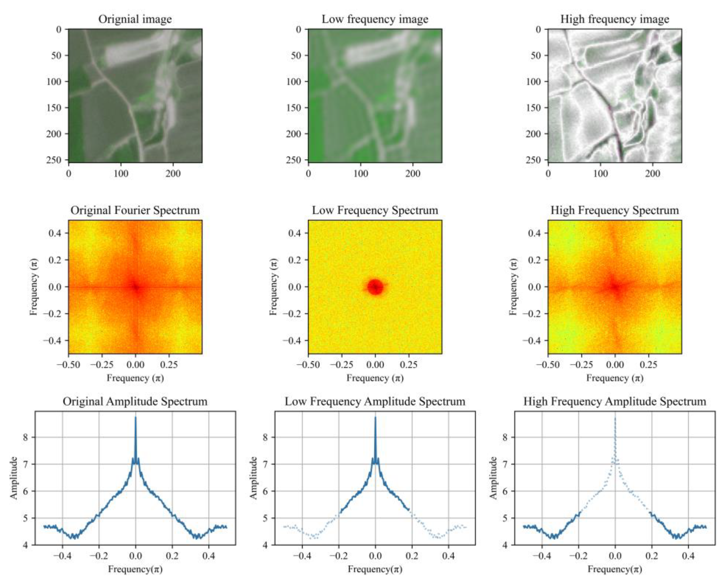
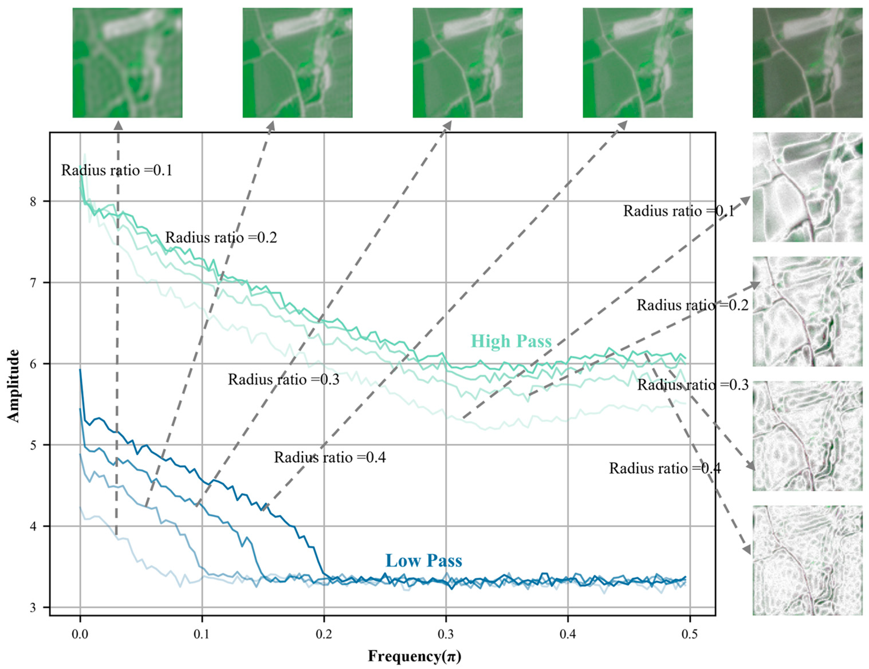
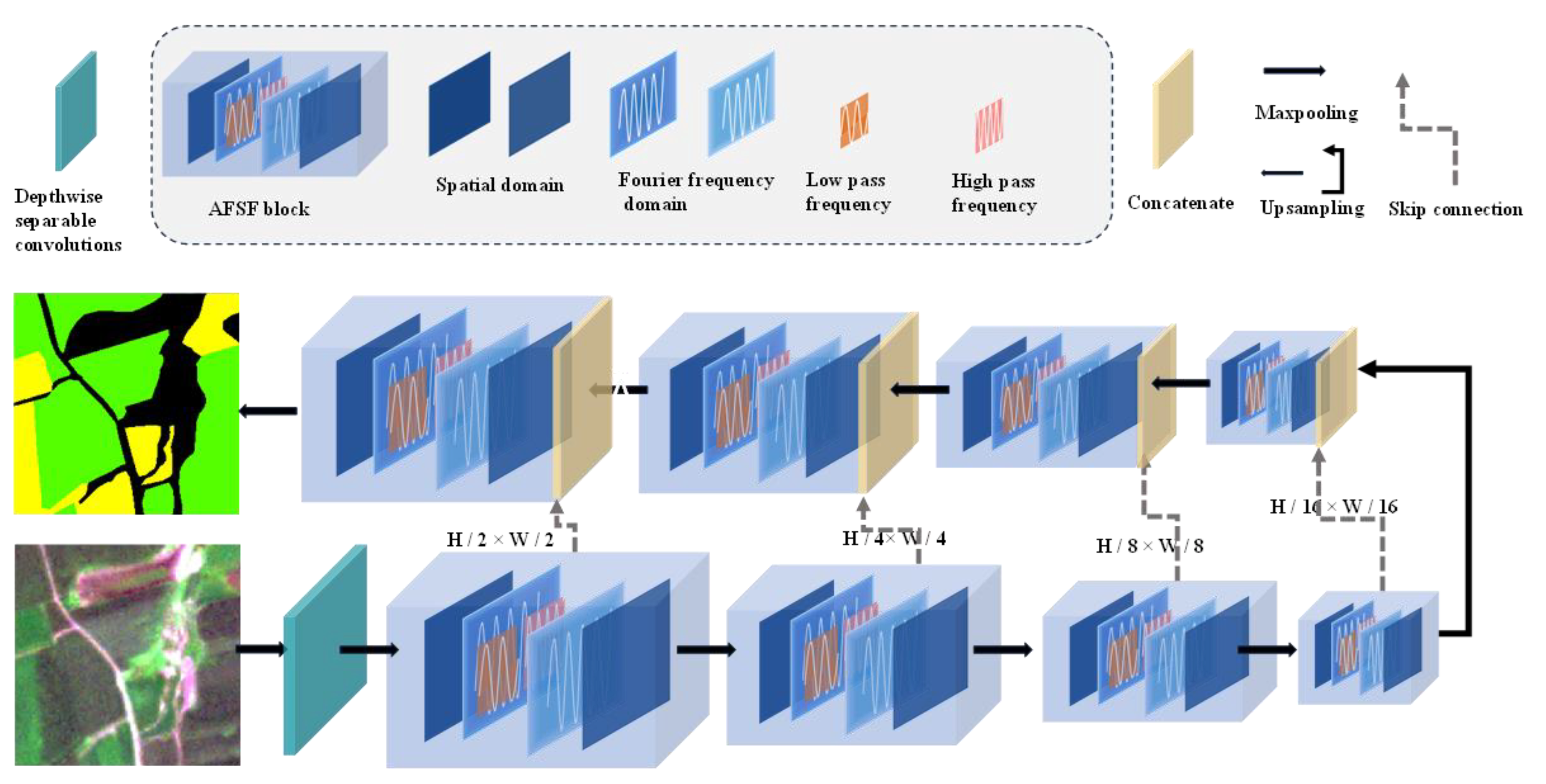
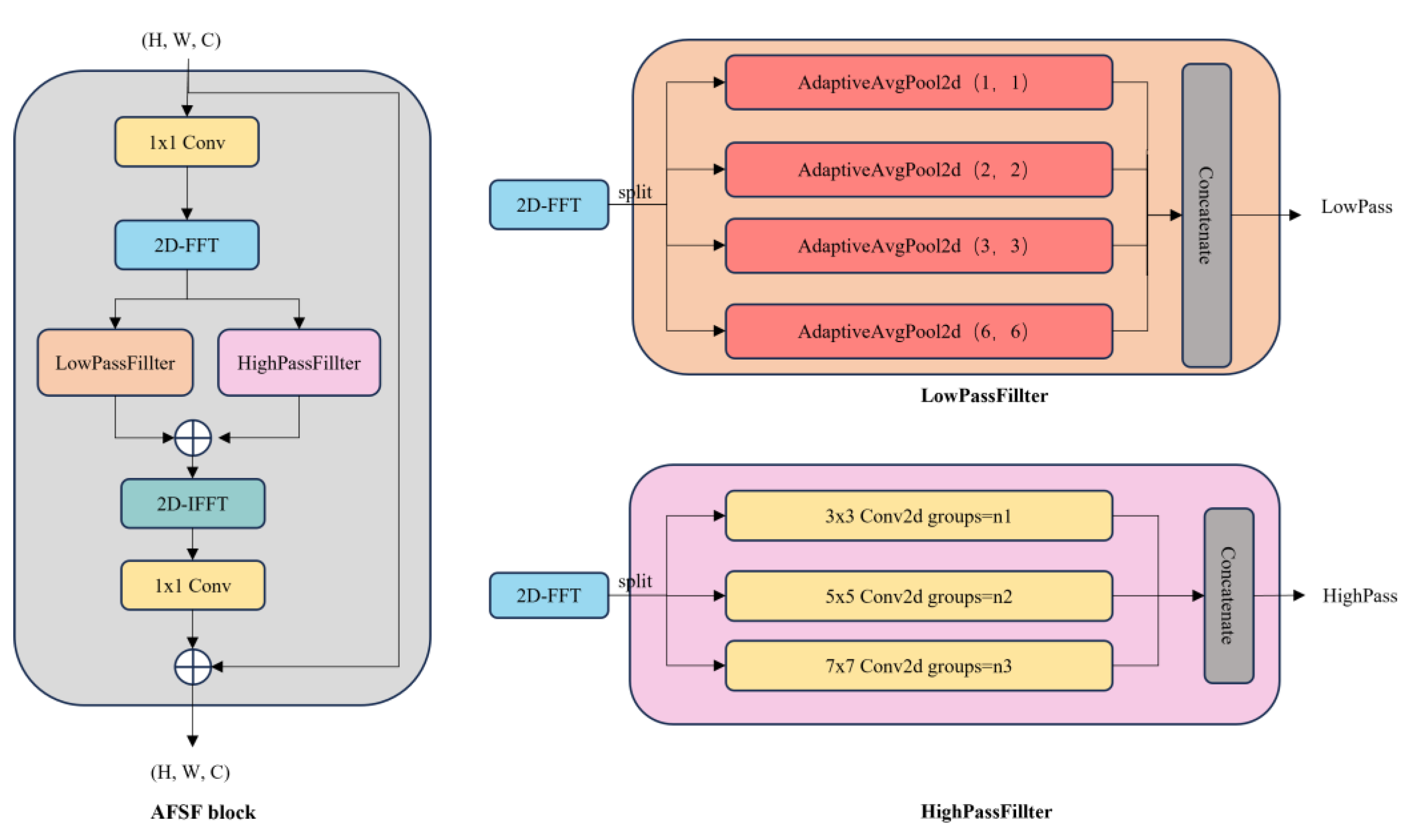
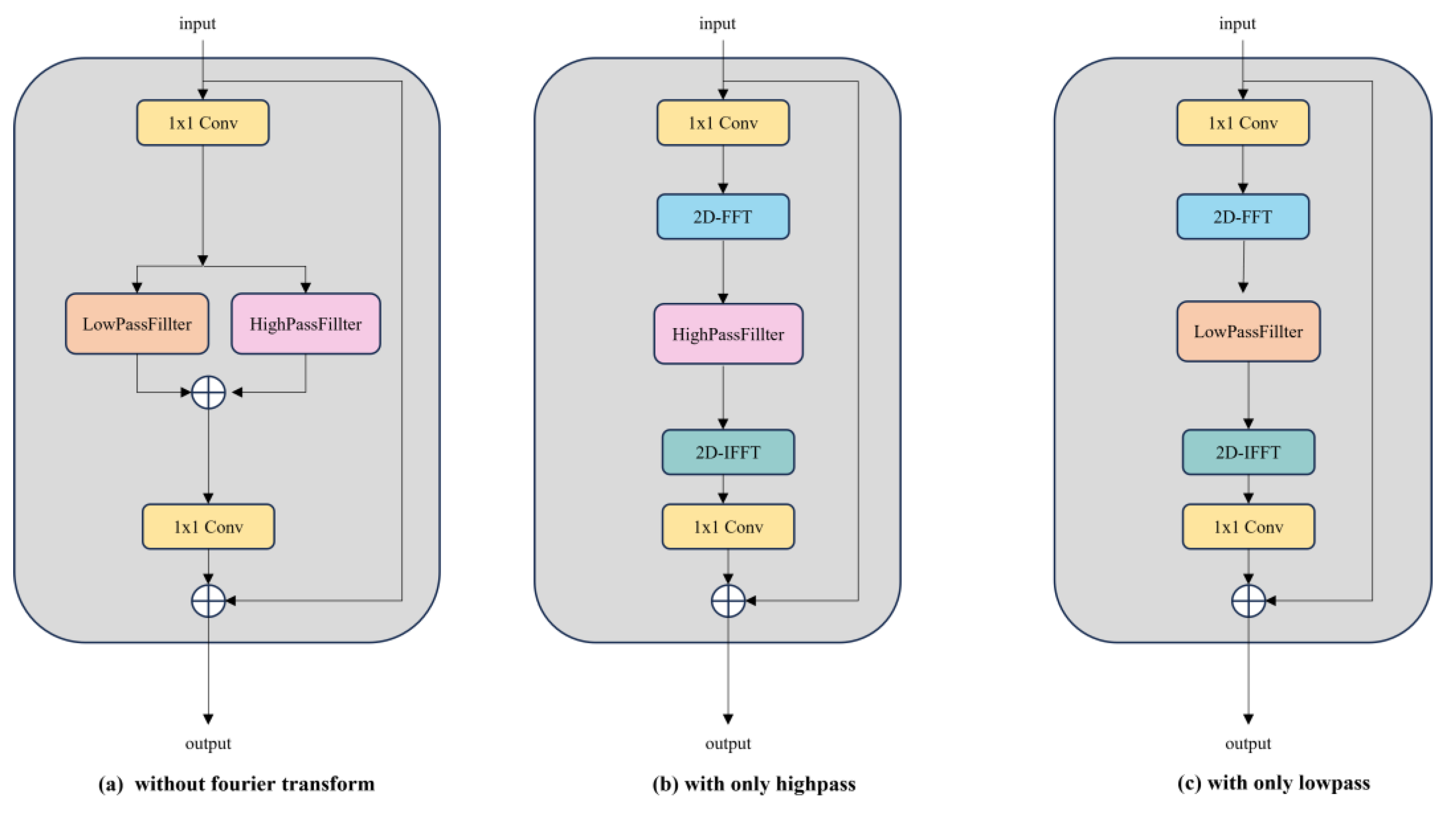
A convolutional neural network based on the Fourier frequency domain learning strategy is proposed, called FFDC net. This approach transforms the feature maps from the spatial domain to the Fourier frequency domain, decomposes the feature maps into low-frequency and high-frequency components in the spectral space using a dynamic frequency filtering component, and automatically adjusts the intensity and distribution of the different frequency components;

(2)

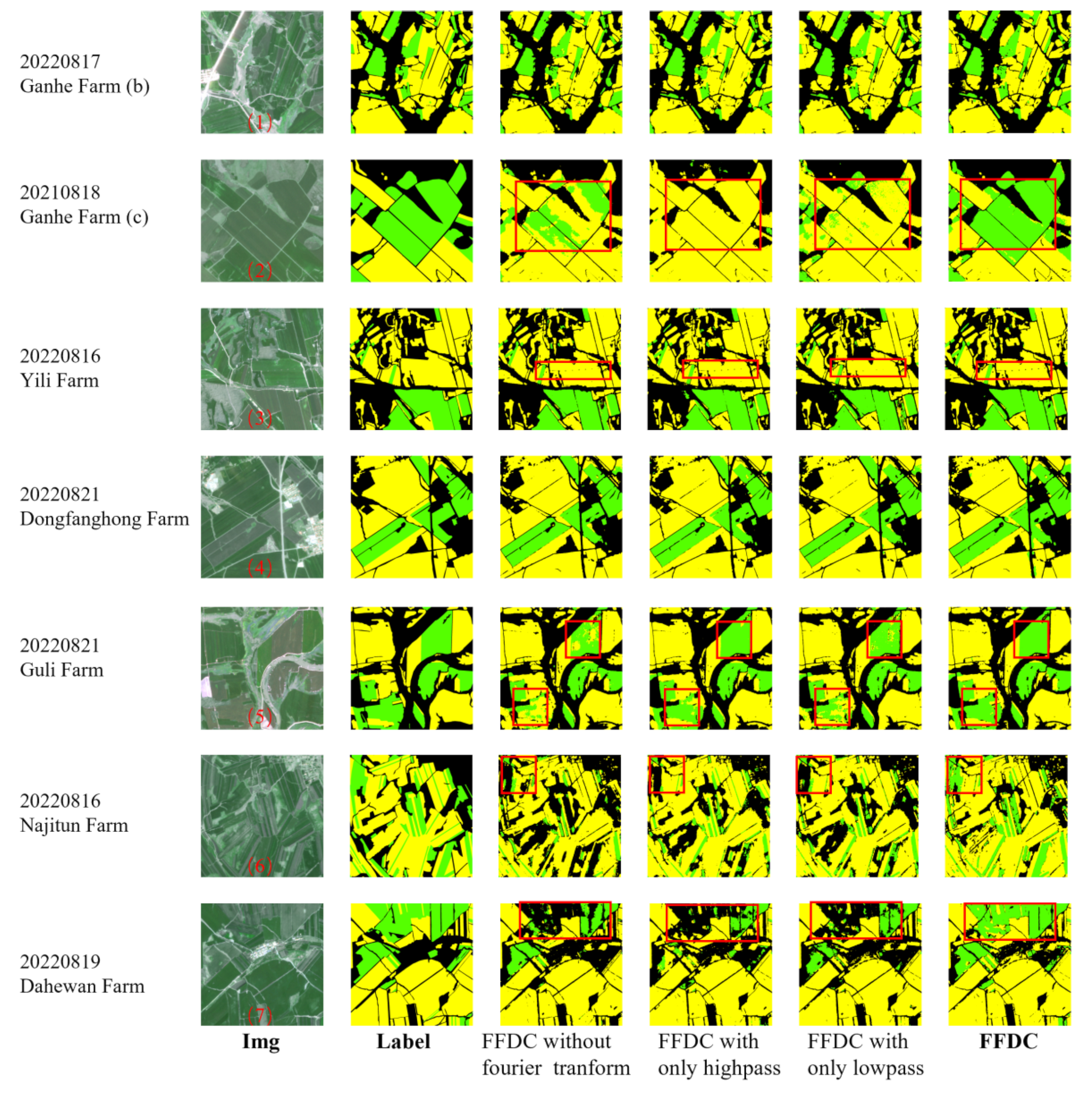
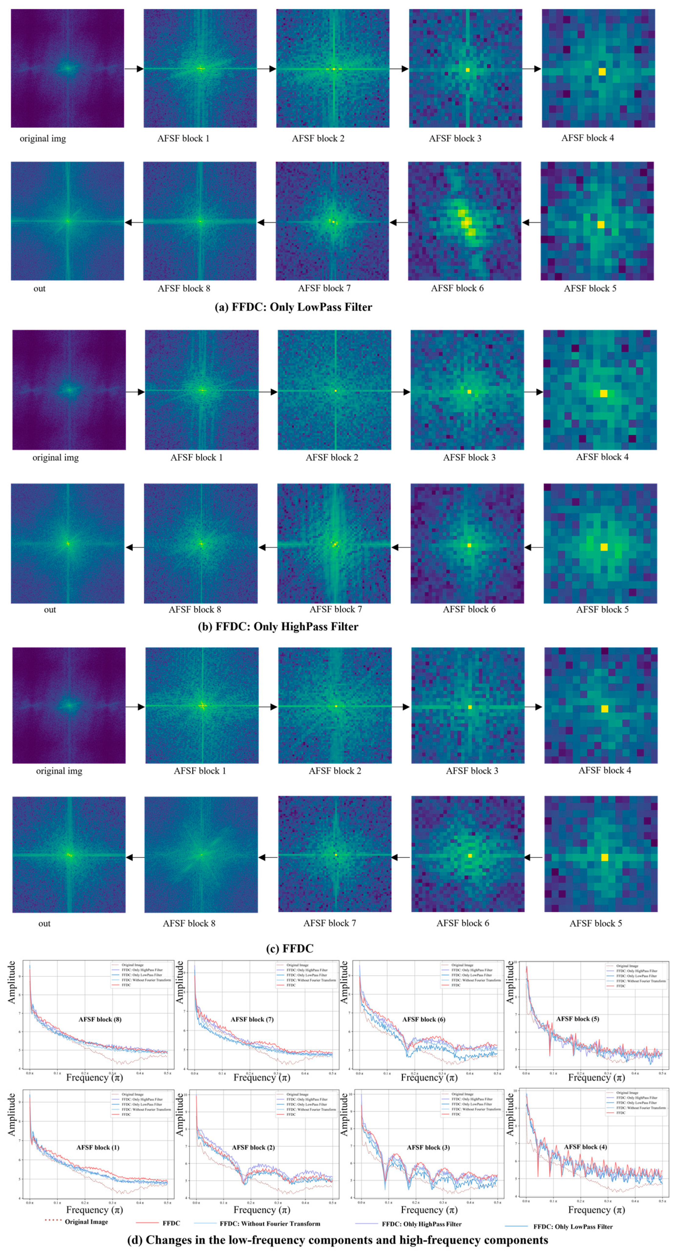
An analysis of the influence of the Fourier frequency domain learning strategy and the Dynamic Frequency Filtering module on the improvement of overall crop classification consistency and boundary distinction in crop classification;

(3)

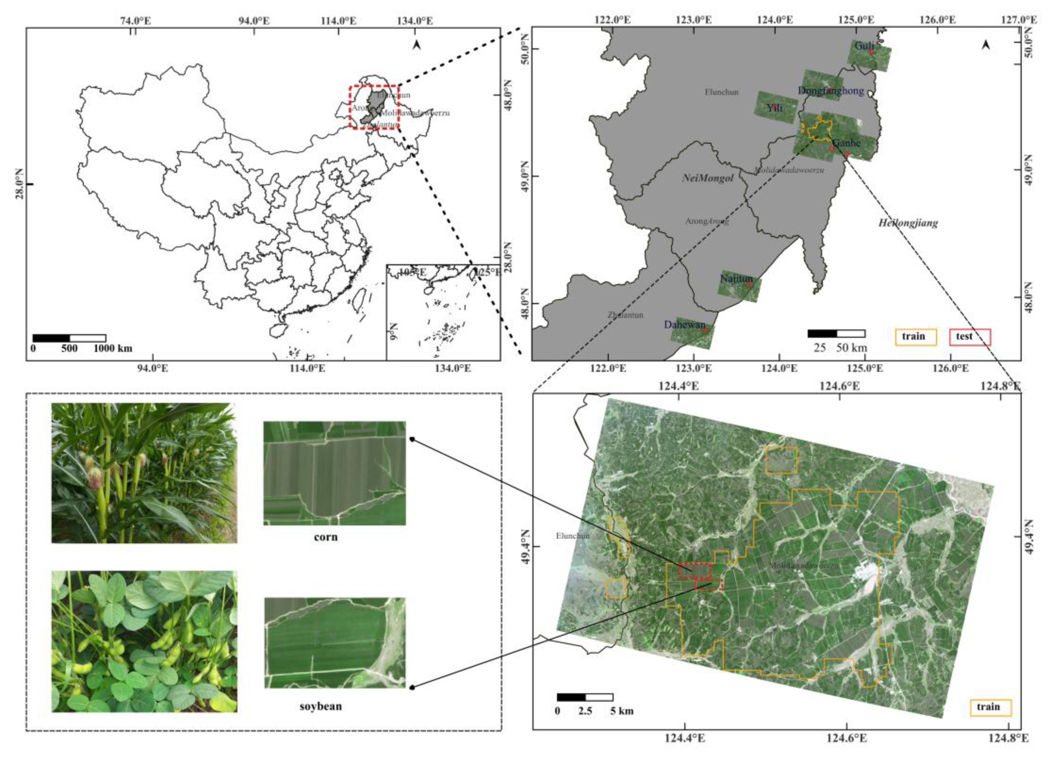
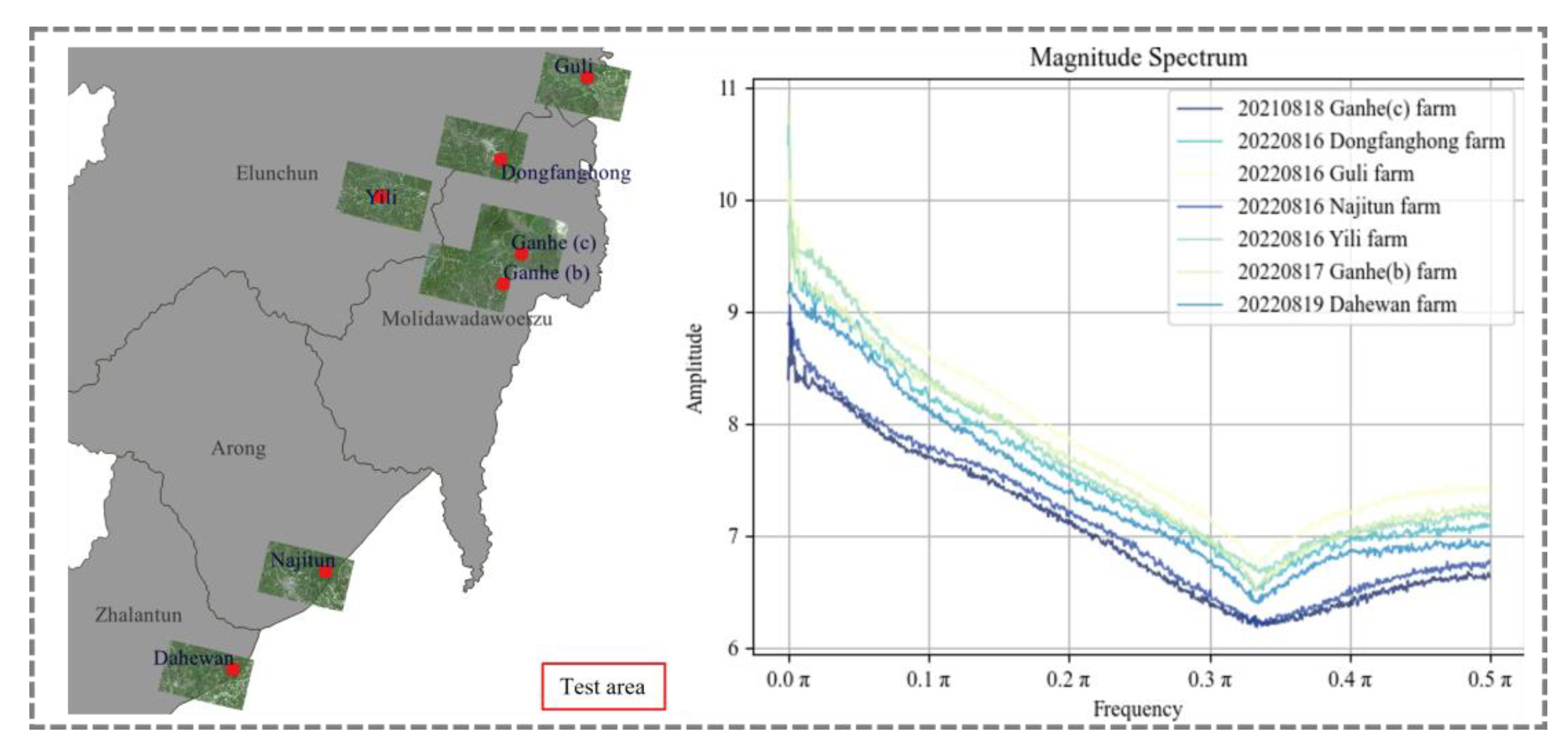
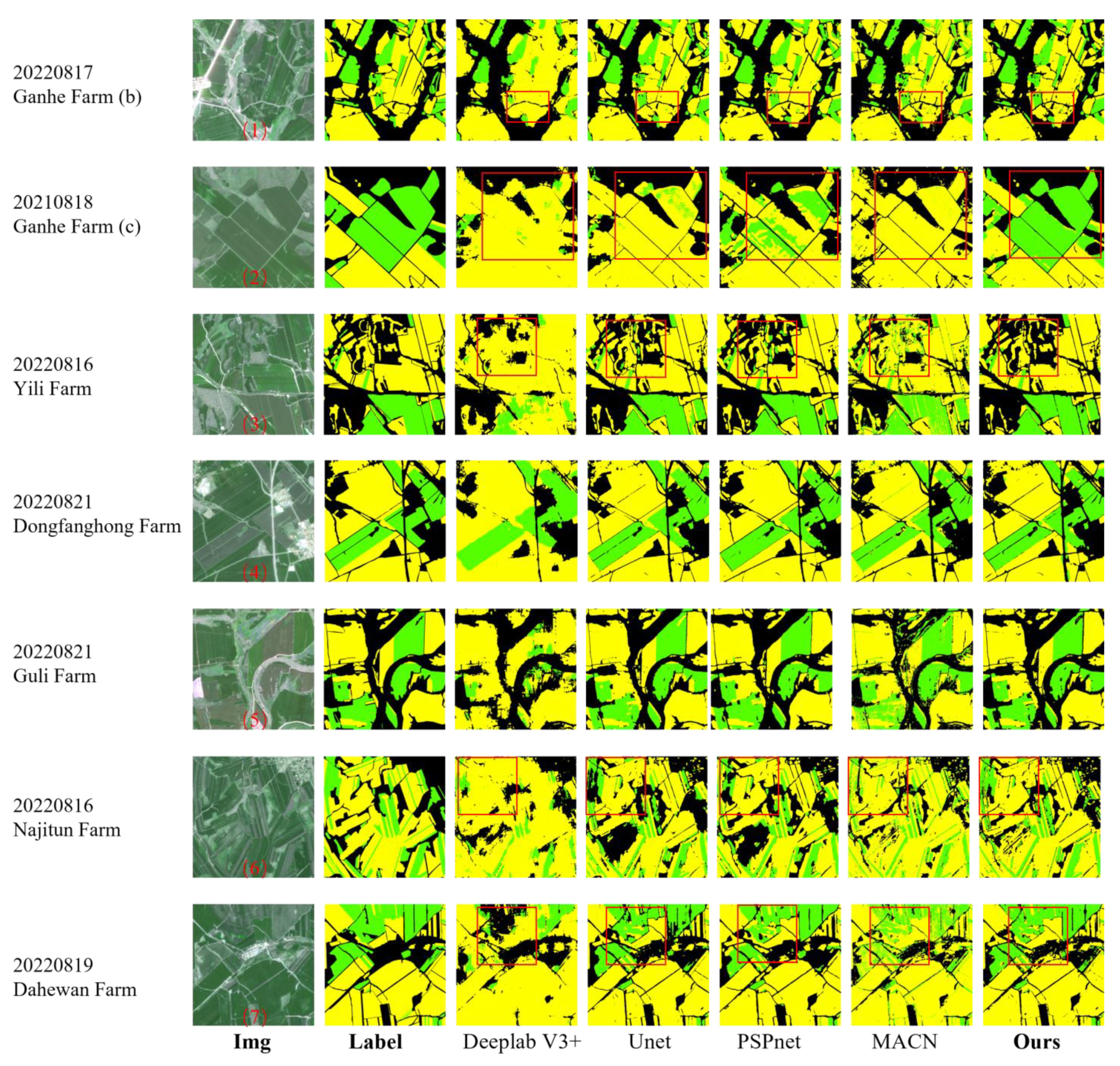
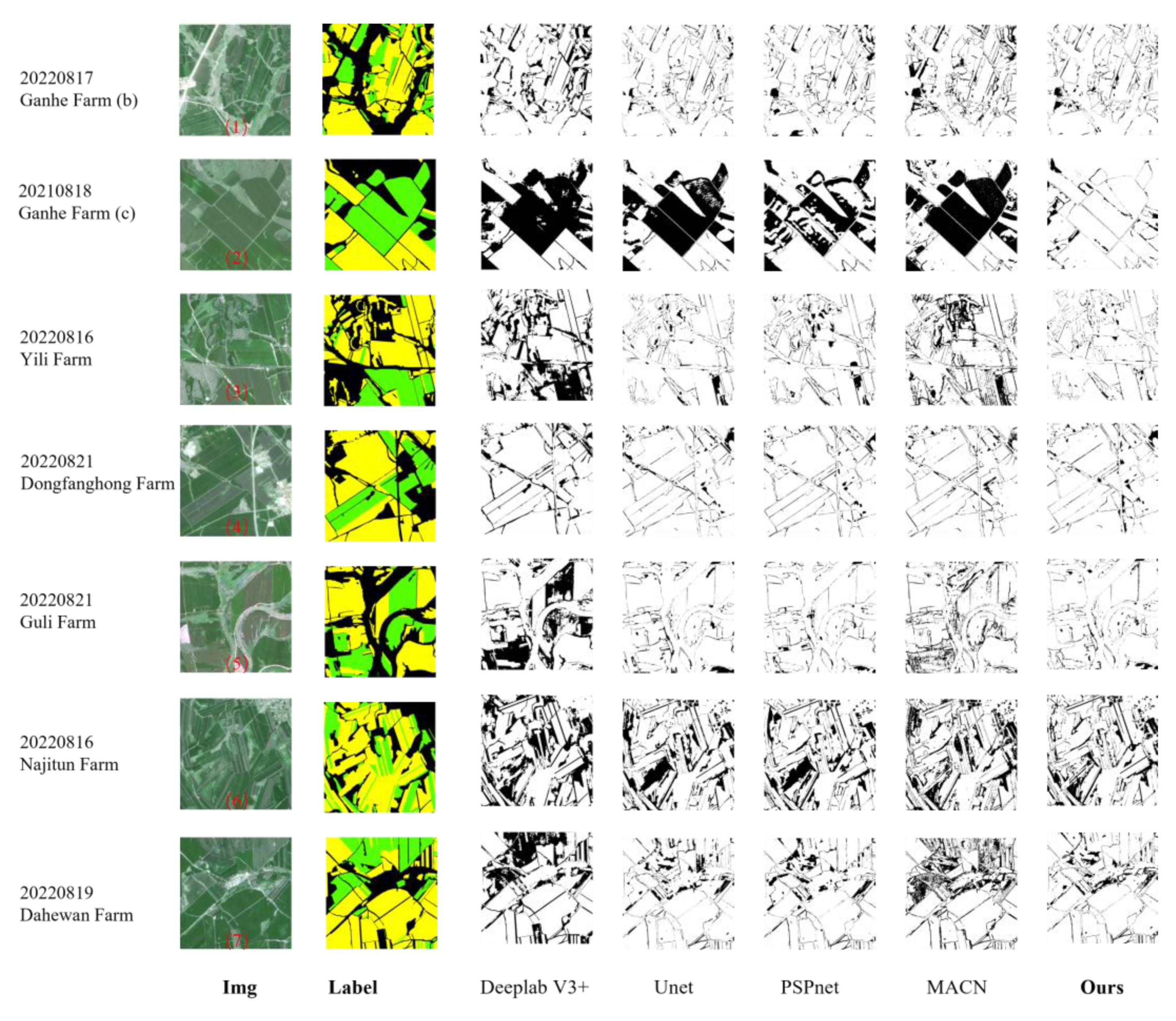
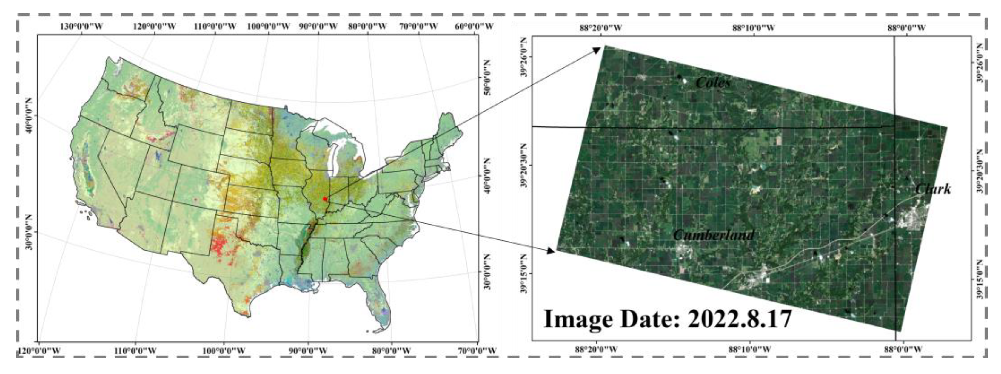
The method’s adaptability was validated and compared through experiments in randomly selected regions from various farms in Hulunbuir, Inner Mongolia, China, and Cumberland County, the USA.

2. Materials and Methods

2.1. Dataset Acquisition and Preprocessing

2.1.1. Study Area

The study area is illustrated in Figure 1 and is comprised of six farms: Ganhe, Guli, Dongfanghong, Yili, Najitun and Dahewan. The training data were primarily collected from the Ganhe farm, while data from the other farms were used for accuracy validation. The Ganhe farm is situated in the transitional sedimentary zone from the southeastern foothills of the Greater Khingan range to the Songnen plain within the territory of the Molidawa Daur autonomous banner. The geographical coordinates of the farm range from approximately 124°18′E to 124°54′E in longitude and 49°9′N to 49°22′N in latitude, with an elevation ranging from 220.0 m to 451.1 m above sea level. The climate of the area falls under the cold temperate continental semi-humid climate zone, with an annual average temperature of 0–0.3 °C, average annual precipitation of 460–500 mm, average annual sunshine hours of 2270 h, effective accumulated temperature of 1900–2100 °C per year and a frost-free period of 105–125 days. The region experiences a single-cropping season suitable for cultivating wheat, soybeans, corn and miscellaneous grains. The climate and crop types in the other farms are similar.

2.1.2. Dataset Acquisition

PlanetScope is a constellation of approximately 130 satellites capable of daily imaging of the entire Earth’s land surface at a resolution of 3 m per pixel. Compared to commonly used data sources, such as Landsat 8, Sentinel-2 and domestic high-resolution data, the PlanetScope data offer unparalleled high temporal resolution and provide abundant spectral and spatial information [43].

Crop classification in remote sensing is influenced by various factors, such as precipitation, soil, climate and management practices, which result in distinct morphological and textural features in the remote sensing images [3]. Using images during specific growth stages can reduce crop classification difficulties. The higher temporal resolution of PlanetScope facilitates the acquisition of crop images at the same growth stage, ensuring consistency in the feature distributions on the remote sensing images and improving the classification accuracy.

The study area, Ganhe farm, mainly cultivates soybeans and corn. The mid-August period is a critical phenological time window for these two crops, during which they exhibit vigorous growth and high distinguishability. Based on the 2022 farm planting plan provided by the local agricultural reclamation company and ground survey data from multiple farms in October 2022, we selected the mid-August 2022 image, Ganhe (a), for Ganhe farm and manually delineated the soybean, corn and background areas as the training dataset. Data collected from images of Yili, Dongfanghong, Guli, Najitun, Dahewan, Dongfanghong, Ganhe (b) and Ganhe (c) were used as the testing dataset. The testing areas cover a wide range, and most were distant from Ganhe Farm, effectively validating the adaptability of the proposed method. By cropping the images, we obtained a total of 2385 samples, each with dimensions of 256 × 256 pixels, with 1908 samples designated for the training dataset and 477 samples for the validation dataset. The image sets used in this paper are presented in

Table 1. The names of the images and the farms involved in the study.

Farm		Image Name
Ganhe	Ganhe (a)	20220817_021446_16_2485_3B_AnalyticMS_SR
	Ganhe (b)	20220817_021723_59_247d_3B_AnalyticMS_SR
	Ganhe (c)	20210818_015304_46_2440_3B_AnalyticMS_SR
Dongfanghong		20220816_023424_19_2405_3B_AnalyticMS_SR
Yili		20220816_022045_11_248c_3B_AnalyticMS_SR
Najitun		20220816_021802_52_2461_3B_AnalyticMS_SR
Guli		20220816_021618_41_2489_3B_AnalyticMS_SR
Dahewan		20220819_021916_67_2484_3B_AnalyticMS_SR

.

2.1.3. Data Preprocessing

In this paper, we utilize the surface reflectance product of PlanetScope imagery, which undergoes orthorectification and radiometric calibration to ensure consistency under local atmospheric conditions and minimize uncertainties in the spectral responses over time and location.

Table 2. PlanetScope 4 Band Dataset Detailed Specifications.

Band No	Band Name	Resolution (m)	Wavelength (nm)
B1	Blue	3	465–515
B2	Green	3	547–593
B3	Red	3	650–680
B4	Nir-infrared	3	845–885

presents the bands, resolution and wavelengths of the PlanetScope imagery. In reference to the image of the Ganhe (a) on 17 August 2022, color balancing was applied to other remote sensing images using ENVI 5.6 software.

2.2. Method

2.2.1. Fourier Transform

In remote sensing, discrete signal representations on raster images can be analyzed and computed using harmonic analysis and spectral graph theory. A Fourier transform is one of the fundamental tools in image signal processing, enabling the decomposition of an image into different frequency components [44]. By utilizing the eigenvectors of the Laplacian matrix as the basis functions for the Fourier transform, any pixel on the remote sensing image can be represented using these basis functions. The Fourier transform transforms the image from the spatial domain to the frequency domain, while the Fourier inverse transform accomplishes the reverse process, as shown in Equations (1) and (2) [45].

$$F\left(u,v\right)={\int }_{-\mathrm{\infty }}^{+\mathrm{\infty }} {\int }_{-\mathrm{\infty }}^{+\mathrm{\infty }} f\left(x,y\right)e^{-j2\pi \left(ux+vy\right)}dxdy$$

(1)

$$f\left(x,y\right)={\int }_{-\mathrm{\infty }}^{\mathrm{\infty }} {\int }_{-\mathrm{\infty }}^{\mathrm{\infty }} F\left(u,v\right)e^{j2\pi \left(ux+vy\right)}dudv$$

(2)

To enhance the computational efficiency of the Fourier transform in computer systems, the fast Fourier transform (FFT) (Equation (3)) and the fast inverse Fourier transform (IFFT) (Equation (4)) are commonly employed in practice.

$$F\left(u,v\right)=\sum _{M_x=0}^{M_x-1} \sum _{M_y=0}^{M_y-1} f\left(x,y\right)e^{-j2\pi \left(\frac{ux}{M_x}+\frac{vy}{M_y}\right)},u,v=\mathrm{0,1},2,\cdots ,Mu-1\mid Mv-1$$

(3)

$$f\left(x,y\right)=\frac{1}{M_u\cdot M_v}\sum _{M_u=0}^{M_u-1} \sum _{M_v=0}^{M_v-1} F\left(u,v\right)e^{-j2\pi \left(\frac{ux}{M_x}+\frac{vy}{M_y}\right)},x,y=\mathrm{0,1},2,\cdots ,Mx-1\mid My-1$$

(4)

As shown in Figure 2, remote sensing images can be decomposed into low-frequency and high-frequency components, similar to natural images. Through a Fourier transform, the remote sensing images are transformed from the spatial domain to the frequency domain. The low-frequency component mainly describes the smoothly varying regions on the homogeneous surface, while the high-frequency component primarily captures rapid changes, such as edges and noise. In other words, the detailed texture information in the image mainly exists in the high-frequency component, while the rich global information is stored in the low-frequency component [45].

Based on the spectral convolution theory in Fourier analysis, modifying a point in the frequency domain can influence the global features in the spatial domain [46]. Therefore, conducting convolutions or other feature extraction operations in the Fourier frequency domain provides a larger receptive field based on the global context. Compared to other convolutional neural networks, this approach exhibits good capabilities in extracting global information, allowing it to capture contextual information from distant locations and thereby improving recognition performance [47].

Figure 3 depicts the relationship between the Fourier domain amplitude and the frequency components for the varying filter radius ratios, along with the corresponding frequency component maps. We observed significant disparities between the low-frequency and high-frequency images obtained with different frequency filter radius ratios [48]. Notably, low-pass filtering with reduced radius ratios leads to image blurring and reduced intraclass differences for the same crop type. Conversely, high-pass filtering preserves the high-frequency components, accentuating the boundaries between the different crop types. Furthermore, increasing the radius ratio amplifies the intraclass differences and reveals more of the textural details within each area. Different land cover types possess distinct frequency-sensitive ranges. Selecting an appropriate filter radius ratio is crucial to balance the edge specificity and internal consistency for the different land cover types.

2.2.2. Network Architecture

Figure 4 illustrates the architecture of the FFDC, which consists of several key components, including depthwise separable convolution (DSC), AFSF blocks, max-pooling layers and skip connections. In the encoding stage, the network utilizes DSC to perform an initial coarse feature extraction while expanding the feature tensor’s channel dimensions. After the DSC, four AFSF modules are applied, each followed by a 2 × 2 max-pooling with a stride of 2. The AFSF modules leverage the dynamic frequency domain filters, which combine the different kernel sizes of the low-pass and high-pass filters. This mechanism effectively filters the unwanted frequency components in the Fourier frequency space, retaining and enhancing the signal within the desired frequency range. Upon transforming back to the image feature space, the AFSF modules integrate the global features from the different channels and the local information of the various scales, thereby emphasizing the meaningful semantic features.

In the decoding stage, the network also employs four AFSF modules, and each decoder subnetwork begins with upsampling to gradually restore the original size of the input image. The use of skip connections enables the fusion of low-level and high-level semantic information, making accurate masks. Additionally, the AFSF blocks from the different encoding layers are connected through skip connections to alleviate the vanishing gradient problem and to capture effective features. Finally, the network utilizes a 1 × 1 convolution to output the multiclass segmentation masks.

2.2.3. Adaptive Frequency Selective Filter Module

Research indicates that the human brain repositions and horizontally processes spatial frequency information between the left and right hemispheres. Notably, different hemispheres exhibit varying levels of activation for distinct frequency components [49]. To emulate this hemisphere-based frequency processing pattern of the human brain, we designed several components in the deep learning network for processing frequency components, namely the low-frequency filter domain and high-frequency filter domain, as illustrated in the right half of Figure 5.

High-frequency information is crucial for retaining segmentation details. Convolution, as a typical multichannel filtering operator, effectively filters out irrelevant low-frequency redundant components while preserving the image edges and contour information [50]. As depicted in the high-pass filters of Figure 5, we divided the channels into N groups and used group convolution layers with different kernels for each group to mimic the cutoff frequencies of the various high-frequency filters. This results in an attenuation of the low-frequency components and a pass of the high-frequency components after high-pass filtering. In contrast, as shown in Figure 2, the low-frequency components carry the majority of the image energy and represent most of the semantic information. To aggregate the different land cover low-frequency component information within the deep learning network, we applied adaptive average pooling with different window sizes as the low-pass filter, ensuring a pass of the low-frequency components and an attenuation of the high-frequency components in the Fourier frequency domain.

Based on the above, we propose an adaptive dynamic filtering module (AFSF), as shown in the left part of Figure 5. By using filters in the frequency domain to enhance or attenuate the strength of each frequency component in the spectrum, the module can effectively reduce the intraclass differences within the same crop type and amplify the interclass differences between the different crop types, thereby improving crop distinguishability.

To reduce the computational complexity, flexibly adjust the dimensions, and facilitate deeper network training, we adopt the bottleneck structure from ResNet [32]. In the bottleneck layer, we utilize a fast Fourier transform to convert the spatial domain tensor to the frequency domain. Smooth internal crop structures are transformed into low-frequency signals, while detailed contours and texture information are transformed into high-frequency signals. We then split the input signal channels into multiple groups, as illustrated in Figure 4. Each channel group represents a specific frequency range. For each group, we apply low-pass and high-pass filtering operations with filters of different sizes. This design allows the module to learn and extract frequency domain features in different frequency ranges, resulting in a richer feature representation. After the low-pass and high-pass filtering, the results of each channel group are merged to perform cross-channel fusion and to reconstruct the frequency domain signal. The merged signal serves as the output of the module, and it is converted back to the spatial domain through an inverse Fourier transform, maintaining the same feature map shape as the input signal.

As frequency domain feature extraction may lead to some loss of the local details, we address this issue by fusing the input as a residual with the output after an inverse Fourier transform. In this way, the AFSF module can fully consider the learning of both the global and local features.

As shown in Figure 6, visualizing the feature maps of the different hierarchical AFSF modules reveals an increasing level of internal consistency and smoothness after multiple rounds of adaptive dynamic filtering, with enhanced boundary delineations.

2.2.4. Training Parameters and Evaluation Metrics

During the training phase, FFDC utilizes the Adam optimizer with an initial learning rate of 1× 10⁻⁴ and a decay rate of 0.5. The batch size is 16, and the total number of training epochs is 60. The research environment for this paper includes Python 3.8, and the deep learning framework used is PyTorch v1.12.1. The model is trained using a 1080ti-11G graphics card for efficient computation.

Dice loss is often used in semantic segmentation tasks to improve the segmentation performance and attenuate the effects of imbalance class problems.

$$\mathrm{D}\mathrm{i}\mathrm{c}\mathrm{e} \mathrm{L}\mathrm{o}\mathrm{s}\mathrm{s}=1-\frac{2\left|\mathrm{X}\cap \mathrm{Y}\right|}{\left|\mathrm{X}\right|+\left|\mathrm{Y}\right|}$$

(5)

where |X⋂Y| is the intersection between the predicted label X and the actual label Y. The |X| and |Y| subtables represent the number of elements of X and Y. The numerator is multiplied by two to ensure that the denominator takes a value in the range of [0, 1] after repeated calculations.

We employ several evaluation metrics, including the mean intersection over union (mIoU), overall accuracy (OA), recall, precision, F1-score and Kappa coefficient, to assess the performance. The F1-score represents the harmonic mean of the precision and recall, providing a comprehensive measure of both the precision and recall. The mIoU reflects the overlap between the predicted values of all the classes and the ground truth boundaries. The Kappa coefficient (Kappa) evaluates the consistency between the predictions and ground truth references, serving as an assessment of the remote sensing interpretation accuracy. To facilitate a comprehensive comparison between FFDC and the other popular models in our experiments, we calculate each of these metrics. The computation formulas for these metrics are as follows:

$$\mathrm{O}\mathrm{A}=\frac{\mathrm{T}\mathrm{P}+\mathrm{T}\mathrm{N}}{\mathrm{T}\mathrm{P}+\mathrm{F}\mathrm{P}+\mathrm{T}\mathrm{N}+\mathrm{F}\mathrm{N}}$$

(6)

$$\mathrm{P}\mathrm{r}\mathrm{e}\mathrm{c}\mathrm{e}\mathrm{s}\mathrm{s}=\frac{\mathrm{T}\mathrm{P}}{\mathrm{T}\mathrm{P}+\mathrm{F}\mathrm{P}}$$

(7)

$$\mathrm{R}\mathrm{e}\mathrm{c}\mathrm{a}\mathrm{l}\mathrm{l}=\frac{\mathrm{T}\mathrm{P}}{\mathrm{T}\mathrm{P}+\mathrm{F}\mathrm{N}}$$

(8)

$$\mathrm{m}\mathrm{I}\mathrm{o}\mathrm{u}=\frac{1}{\mathrm{k}+1}\sum _{\mathrm{i}=0}^{\mathrm{k}}\frac{\mathrm{T}\mathrm{P}}{\mathrm{T}\mathrm{P}+\mathrm{F}\mathrm{P}+\mathrm{F}\mathrm{N}}$$

(9)

$$\mathrm{F}1=\frac{2\mathrm{T}\mathrm{P}}{2\mathrm{T}\mathrm{P}+\mathrm{F}\mathrm{P}+\mathrm{F}\mathrm{N}}$$

(10)

$${\mathrm{p}}_{\mathrm{e}}=\frac{\left(\mathrm{T}\mathrm{P}+\mathrm{F}\mathrm{P}\right)·\left(\mathrm{T}\mathrm{P}+\mathrm{F}\mathrm{N}\right)+\left(\mathrm{T}\mathrm{N}+\mathrm{F}\mathrm{P}\right)·\left(\mathrm{T}\mathrm{N}+\mathrm{F}\mathrm{N}\right)}{{\left(\mathrm{T}\mathrm{P}+\mathrm{F}\mathrm{P}+\mathrm{T}\mathrm{N}+\mathrm{F}\mathrm{N}\right)}^2}$$

(11)

$$\mathrm{K}\mathrm{a}\mathrm{p}\mathrm{p}\mathrm{a}=\frac{\mathrm{O}\mathrm{A}-{\mathrm{p}}_{\mathrm{e}}}{1-{\mathrm{p}}_{\mathrm{e}}}$$

(12)

where True Positive (TP) and True Negative (TN) represent the number of pixels correctly predicted as positive and negative classes, respectively. False-positive (FP) and false-negative (FN) represent the number of nonobject pixels incorrectly classified as positive and the number of object pixels incorrectly classified as negative, respectively.

In addition, the number of parameters (Params) and floating point operations (FLOPs) are also used to evaluate the arithmetic consumption and size of the model and the size of the model, as well as the importance of the proposed modules.

3. Results

In the past decade, numerous deep-learning methods have emerged for remote sensing crop recognition. These methods include, but are not limited to, Convolutional Neural Networks [51], cellular neural networks [52], Contextual deep CNN [53], FCN [54], U-Net [18], CENN [55], U-Net++ [19], PSPnet [20], SegNet [22], MACNnet [12] and DeeplabV3+ [21], HyFormer [35] and CTFuseNet [37]. Among them, U-Net [19], DeepLab V3+ [21], and PSPnet [20] are widely used and highly representative segmentation methods and many improved methods are based on these. Additionally, MACNnet [12] stands out as a relatively novel and excellent classification method.

To validate the effectiveness of FFDC, we conduct comparative analyses with U-Net [18], DeepLab V3+ [21], PSPnet [20] and MACNnet [12]. In this paper, we randomly select seven regions from six farms to evaluate the model’s performance. These seven farm regions are spatially distributed from south to north, collected from different images, and exhibit relatively complex planting structures. The spatial distribution and frequency domain variations of the seven test regions are illustrated in Figure 7.

Figure 8 shows the classification results in the seven validation regions. From Figure 8, it can be observed that all five deep-learning models demonstrate certain capabilities for soybean and corn recognition in the different validation regions; however, the classification results exhibit significant differences. The ordering of Figure 8(1–7) in Figure 8 indicates the distance from the test dataset to the sample collection area, which ranges from close to far. As the distance from the sample collection location at the Ganhe farm increases, the generalization performance of the models gradually decreases, leading to a decline in the accuracy and completeness of the extractions. However, the red rectangular boxes clearly indicate that our model consistently achieves better results in terms of intrafield consistency and boundary accuracy.

In Figure 8(1), the farm region is closest to the training data location, both being at Ganhe Farm. All five models exhibit good crop extraction results, accurately and completely identifying soybean and corn. Figure 8(3–5) are at similar distances from Ganhe Farm with comparable complexities in planting structures. The five models maintain high crop interior consistency and boundary accuracy in these regions. Figure 8(6,7) are more remote from the Ganhe farm, with significantly higher complexities in the planting structures compared to the previous farms. In these regions, the performance of FFDC also declines, but its results in terms of intrafield consistency, completeness and boundary fit are superior to those of the other models. Figure 8(2) shows the extraction results of various models on the 2021 Ganhe Farm Planetscope images. U-Net, DeeplabV3+ and MACNnet misidentify corn as soybean, while FFDCnet correctly identifies it as corn. This demonstrates that FFDCnet maintains high intrafield consistency and boundary accuracy for the same growth stage across different years, indicating its strong temporal transferability capabilities.

The difference visualizations effectively demonstrate the extraction capabilities of the models. Figure 9 displays the difference visualizations of the extraction results from the seven test regions. The black areas represent misidentified regions, and a higher proportion of black indicates a poorer model performance. From Figure 9, it is evident that FFDCnet has the lowest proportion of black areas, surpassing all the comparative methods. It exhibits the best performance with the most accurate identification, better boundary fit with crop image boundaries, a more complete internal structure and fewer fragmented areas. This strongly validates that our proposed method achieves superior intrafield consistency and boundary accuracy in the extraction results.

To further demonstrate the accuracy improvement achieved by our proposed method, we perform quantitative statistics on the seven regions, separately using precision, recall, F1, OA, mIo and the Kappa coefficient.

Table 3. The average accuracy of each method was evaluated in seven test regions.

Method	Precision		Recall		F1		OA	mIoU	Kappa	Flops	Params
	Corn	Soybean	Corn	Soybean	Corn	Soybean
DeeplabV3+	0.9607	0.3606	0.6752	0.8741	0.7930	0.5106	0.7331	0.5289	0.5543	7.9 G	5.2 M
U-Net	0.9446	0.6720	0.8178	0.9093	0.8766	0.7728	0.8525	0.7236	0.7633	50.8 G	32.1 M
PSPnet	0.9221	0.7509	0.8570	0.8881	0.8883	0.8138	0.8622	0.7437	0.7814	50.5 G	52.5 M
MACN	0.9425	0.5850	0.7562	0.8076	0.8391	0.6785	0.7990	0.6381	0.6742	20.3 G	17.2 M
FFDC	0.9432	0.8936	0.9084	0.9369	0.9255	0.9147	0.9092	0.8305	0.8571	7.5 G	2.62 M

presents the quantitative statistical results of the five models in the 7 test regions. Comparing the six metrics, it can be observed that FFDC consistently outperforms DeeplabV3+, U-Net, PSPnet and MACN in terms of average recall, F1, mIoU and Kappa coefficient.

For soybean and corn, FFDC achieves an average recall of 0.9084 and 0.9369, 5% and 2%, respectively, which are higher than PSPnet, the best model in the other comparison methods. Similarly, the average F1 scores of FFDC are 0.9255 and 0.9147, which are 3% and 10% higher than those of PSPnet, respectively. Furthermore, the average OA, mIoU and Kappa coefficient of FFDC are 0.9092, 0.8305 and 0.8571, which are higher by 4.7%, 8.67% and 7.57%, respectively. These evaluation metrics effectively indicate that spectrum feature learning can significantly enhance the accuracy of the classification results.

FLOPs and Params in Table 3 clearly demonstrate that FFDCnet has the lowest computational complexity and the fewest parameters compared to other models, with only 7.5 G and 2.62 M, respectively. This can be attributed to the design of channel splitting with frequency-domain filters to capture different frequency-domain features. The increased channel splitting significantly reduces the model’s complexity and its demand for computational resources.

4. Discussion

To further investigate the effectiveness of frequency domain learning, low-pass filtering and high-pass filtering on crop classification, as well as the validity of the model design, we conduct three ablation experiments. Figure 10 illustrates the AFSF module structures with the removal of the Fourier transform strategy, low-pass filter and high-pass filter. Figure 11 presents the crop classification results of the three ablation experiments, and

Table 4. Evaluation of the accuracy of the ablation experiments.

Ablation	Precision		Recall		F1		OA	mIoU	Kappa	FLOPs	Params
	Corn	Soybean	Corn	Soybean	Corn	Soybean
Only low-pass	0.9344	0.5940	0.8421	0.9375	0.8858	0.7272	0.8479	0.7048	0.7548	4.13 G	1.26 M
Only high-pass	0.9378	0.5605	0.8193	0.9496	0.8746	0.7049	0.8368	0.6860	0.7356	4.25 G	1.32 M
No Fourier	0.9221	0.6186	0.8558	0.9502	0.8877	0.7494	0.8476	0.7082	0.7553	4.18 G	1.27 M
FFDC	0.9432	0.8936	0.9084	0.9369	0.9255	0.9147	0.9092	0.8305	0.8571	7.54 G	2.62 M

shows the quantitative accuracy evaluation results of the three ablation experiments in the seven validation farmland regions.

To verify the effectiveness of frequency learning, we conduct the first set of ablation experiments by removing the Fourier transform from the AFSF module, as shown in Figure 10a. From the red rectangular boxes in Figure 11(2,5–7), it is evident that the FFDC without the Fourier transform produces many misclassifications, internal fragmentation and incomplete boundaries in soybean and maize identification. Table 4 shows that the overall accuracy of the seven evaluation regions decreases from 0.8949 to 0.8476, mIoU decreases from 0.8109 to 0.7082, and Kappa coefficients decrease from 0.8347 to 0.7553. This indicates that the Fourier frequency transform and frequency learning strategy can improve crop classification performance.

Furthermore, as indicated by Params and FLOPs in Table 4, converting spatial-domain features to the Fourier frequency domain effectively reduces the number of model parameters and computational complexity. FLOPs decrease significantly from 7.54 G to 4.18 G, and Params decrease from 2.62 M to 1.27 M, reducing them by approximately half. However, removing the low-pass filter or high-pass filter while substantially reducing the number of parameters and computational complexity also impairs the model’s performance. Therefore, Fourier transform, low-pass filter, and high-pass filter are crucial for FFDCnet’s performance.

To investigate the performance of the frequency filters, we conduct the second and third sets of ablation experiments by removing the high-pass filter and low-pass filter, respectively, as shown in Figure 10b,c. From the red rectangular boxes in Figure 11, it can be observed that removing either the low-pass or high-pass filter results in more internal fragmentation, incomplete recognition and classification errors compared to FFDCnet. The quantitative accuracy evaluation in Table 4 shows that in the absence of either the low-pass or high-pass filter, the overall accuracy, mIoU and Kappa coefficients of the seven evaluation regions all exhibit varying degrees of decline. After removing the low-pass filter, the overall accuracy of the seven evaluation regions decreased from 0.8949 to 0.8368, mIoU decreased from 0.8109 to 0.6860, and the Kappa coefficients decreased from 0.8347 to 0.7536. After removing the high-pass filter, the overall accuracy of the seven evaluation regions decreased from 0.8949 to 0.8479, mIoU decreased from 0.8109 to 0.7038, and the Kappa coefficients decreased from 0.8347 to 0.7548, even performing worse than the other models. Therefore, it can be concluded that solely learning the low-frequency or high-frequency information of the image leads to internal fragmentation and incomplete boundaries in regions with complex crop structures. Both the high-pass and low-pass filters are indispensable components of FFDC, playing a crucial role in maintaining internal consistency and boundary delineation accuracy.

In addition, from Figure 11(2) of the ablation experiments in Figure 11, it can be observed that the FFDC, which combines both high-frequency and low-frequency information, can better identify soybean and maize in the region of the 2021 year. However, FFDC with only high-frequency or low-frequency information tends to misclassify most of the maize as soybean, as shown in Figure 11(6,7), indicating that FFDC with only high-frequency or low-frequency information mistakenly identifies most of the maize within the red boxes as the background. Therefore, in regions with large time spans, inconsistent crop growth and complex planting structures, the accurate identification of soybean and maize can only be achieved by combining both the high-pass and low-pass filter features.

To further elucidate the underlying frequency learning principles, we visualized the frequency features of the feature tensors outputted by each AFSF module in the network. Figure 12a–c presents the Fourier spectrum of the network at different AFSF blocks, while Figure 12d shows the projection of the frequency domain output of the different AFSF modules in the length direction to demonstrate the variations in the low-frequency and high-frequency components at the different stages of the network.

Upon examining Figure 12a,b,d, it becomes evident that as the network deepens, the low-pass filter strengthens the low-frequency components compared to the Fourier spectrum distribution of the original image, while the high-pass filter reinforces the high-frequency components, showing its powerful filtering capabilities. Furthermore, it can be seen from Figure 12c,d that the AFSF module, which combines the high-frequency and low-frequency information, recombines and enhances certain frequency components, primarily focusing on the high-frequency portion. Compared to only using high-pass filters, this approach produces increased saturation on the high-frequency components, likely because in the crop segmentation tasks, the boundary and texture differences of the crops play a crucial role in object identification [48]. Simultaneously, learning the low-frequency information also improves the network’s robustness against interfering factors [56,57].

Through the aforementioned validation and analysis, we observe that Fourier frequency transformation enhances the deep learning neural network’s ability to capture the complex features of agricultural crops. The dynamic filtering component strengthens the expression of the high-frequency information corresponding to the different crops in the remote sensing images, thereby expanding the capture of the interclass differential features among the crops. It also enhances the consistency of the low-frequency information within the same crops in the remote sensing images, contributing to better preservation of the integrity of the identified crop plots and the accuracy of their boundaries.

To further validate the robustness of our method, we utilize the trained FFDCnet model and randomly selected the Cumberland region for crop extraction, which is located in the main soybean and corn production region of the United States. Figure 13 represents the location of the Cumberland region and the corresponding images used.

The United States cultivates the same staple crops, such as soybeans and corn, as Northeast China and shares a similar phenological cycle. To assess FFDCnet’s performance, we utilized a PlanetScope image captured concurrently with the Ganhe farm (a) in China. The labels presented in Figure 14 were generated using the 2022 Cropland Date Layer (CDL) date from the United States. From the extraction results depicted in Figure 14, it is evident that FFDCnet excels at extracting soybeans and corn in the Cumberland County region despite the geographical distance from China.

Table 5. Evaluation of the accuracy of extraction results in Cumberland County.

Method	OA	mIoU	Kappa
DeeplabV3+	0.7466	0.5192	0.6145
U-Net	0.7894	0.6565	0.6897
PSPnet	0.8072	0.6548	0.6854
MACN	0.7214	0.5080	0.5974
FFDC	0.8466	0.7184	0.7967

provides an overview of the accuracy evaluation results. In comparison to the CDL data, FFDCnet exhibits an OA of 0.8466, a mIoU of 0.7184, and a Kappa coefficient of 0.7967. These metrics confirm FFDCnet’s superior extraction performance compared to the other four models, highlighting its robustness within the same phenological period between Hulunbuir, Inner Mongolia, and Cumberland County, USA.

5. Conclusions

In this paper, our aim is to reduce the high-precision crop classification in high-resolution remote sensing image challenges, such as internal fragmentations, discontinuous boundaries and misclassifications. We propose a novel convolutional neural network based on Fourier frequency domain learning, called FFDCnet, and the network is applied to extract soybean and maize from PlanetScope images in the Hulunbuir region of Northeast China. In the FFDCnet, we employ a Fourier transform strategy and adaptive dynamic filters to construct the adaptive frequency spectral filtering (AFSF) module. This module converts the feature maps into the frequency spectral domain, which contains both low-frequency and high-frequency information. By utilizing low-pass and high-pass filters with different kernel sizes, we separate the low-frequency components, representing the global crop information, and the high-frequency components, representing the edge information. This process captures the frequency features of the different scales for various crops and dynamically adjusts them, obtaining enhanced or attenuated frequency components to improve the information expression of the high-frequency components among the different crops and reduce the distribution differences of the low-frequency components within the same crop, thereby enhancing the overall performance. The soybean and maize extraction results from validation regions in Hulunbuir, Inner Mongolia and Cumberland County, using PlanetScope images, demonstrate that our FFDCnet outperforms the other deep learning models (U-Net, DeepLab V3+, PSPnet and MACN) in terms of capturing internal crop completeness and boundary accuracy, with OA, mIoU and the Kappa coefficients reaching 0.8949, 0.8109 and 0.8347, respectively. The ablation experiments further explain and validate the frequency-based feature learning and description in the FFDCnet, which enhances the separability among the different crops and significantly alleviates common remote sensing crop classification issues, such as crop misclassifications, incomplete intraplot information, fragmented boundaries and poor model generalization across regions, thus significantly improving the performance of the deep learning model. The proposed method provides a new and effective approach for generating accurate and intelligent agricultural production statistics across global land areas.

References

1. MacDonald, R.B.; Hall, F.G. Global Crop Forecasting. Science 1980, 208, 670–679. [Google Scholar] [CrossRef] [PubMed]
2. Potgieter, A.B.; Zhao, Y.; Zarco-Tejada, P.J.; Chenu, K.; Zhang, Y.; Porker, K.; Biddulph, B.; Dang, Y.P.; Neale, T.; Roosta, F.; et al. Evolution and application of digital technologies to predict crop type and crop phenology in agriculture. In Silico Plants 2021, 3, diab017. [Google Scholar] [CrossRef]
3. Weiss, M.; Jacob, F.; Duveiller, G. Remote sensing for agricultural applications: A meta-review. Remote Sens. Environ. 2020, 236, 111402. [Google Scholar] [CrossRef]
4. Luo, Z.; Yang, W.; Yuan, Y.; Gou, R.; Li, X. Semantic segmentation of agricultural images: A survey. Inf. Process. Agric. 2023; in press. [Google Scholar] [CrossRef]
5. Muruganantham, P.; Wibowo, S.; Grandhi, S.; Samrat, N.H.; Islam, N. A Systematic Literature Review on Crop Yield Prediction with Deep Learning and Remote Sensing. Remote Sens. 2022, 14, 1990. [Google Scholar] [CrossRef]
6. Ennouri, K.; Kallel, A. Remote Sensing: An Advanced Technique for Crop Condition Assessment. Math. Probl. Eng. 2019, 2019, 9404565. [Google Scholar] [CrossRef]
7. Hashemi-Beni, L.; Gebrehiwot, A. Deep learning for remote sensing image classification for agriculture applications. Int. Arch. Photogramm. Remote Sens. Spat. Inf. Sci. 2020, XLIV-M-2-2, 51–54. [Google Scholar] [CrossRef]
8. Wu, B.; Zhang, M.; Zeng, H.; Tian, F.; Potgieter, A.B.; Qin, X.; Yan, N.; Chang, S.; Zhao, Y.; Dong, Q.; et al. Challenges and opportunities in remote sensing-based crop monitoring: A review. Natl. Sci. Rev. 2022, 10, nwac290. [Google Scholar] [CrossRef] [PubMed]
9. Kattenborn, T.; Leitloff, J.; Schiefer, F.; Hinz, S. Review on Convolutional Neural Networks (CNN) in vegetation remote sensing. ISPRS J. Photogramm. Remote Sens. 2021, 173, 24–49. [Google Scholar] [CrossRef]
10. Bhatt, D.; Patel, C.; Talsania, H.; Patel, J.; Vaghela, R.; Pandya, S.; Modi, K.; Ghayvat, H. CNN Variants for Computer Vision: History, Architecture, Application, Challenges and Future Scope. Electronics 2021, 10, 2470. [Google Scholar] [CrossRef]
11. Wu, Y.; Wu, P.; Wu, Y.; Yang, H.; Wang, B. Remote Sensing Crop Recognition by Coupling Phenological Features and Off-Center Bayesian Deep Learning. Remote Sens. 2023, 15, 674. [Google Scholar] [CrossRef]
12. Wu, Y.; Wu, Y.; Wang, B.; Yang, H. A Remote Sensing Method for Crop Mapping Based on Multiscale Neighborhood Feature Extraction. Remote Sens. 2022, 15, 47. [Google Scholar] [CrossRef]
13. Yuan, X.; Shi, J.; Gu, L. A review of deep learning methods for semantic segmentation of remote sensing imagery. Expert Syst. Appl. 2021, 169, 114417. [Google Scholar] [CrossRef]
14. Anilkumar, P.; Venugopal, P. Research Contribution and Comprehensive Review towards the Semantic Segmentation of Aerial Images Using Deep Learning Techniques. Secur. Commun. Netw. 2022, 2022, 6010912. [Google Scholar] [CrossRef]
15. Shelhamer, E.; Long, J.; Darrell, T. Fully convolutional networks for semantic segmentation. In Proceedings of the IEEE Conference on Computer Vision and Pattern Recognition, Boston, MA, USA, 7–12 June 2015. [Google Scholar] [CrossRef]
16. Hong, Q.; Yang, T.; Li, B. A Survey on Crop Image Segmentation Methods. In Proceedings of the 8th International Conference on Intelligent Systems and Image Processing 2021, Kobe, Japan, 6–10 September 2021; pp. 37–44. [Google Scholar] [CrossRef]
17. Zhou, Z.; Li, S.; Shao, Y. Crops classification from sentinel-2a multi-spectral remote sensing images based on convolutional neural networks. In Proceedings of the IGARSS 2018–2018 IEEE International Geoscience and Remote Sensing Symposium, Valencia, Spain, 22–27 July 2018. [Google Scholar] [CrossRef]
18. Zou, J.; Dado, W.T.; Pan, R. Early Crop Type Image Segmentation from Satellite Radar Imagery. 2020. Available online: https://api.semanticscholar.org/CorpusID:234353421 (accessed on 18 June 2023).
19. Wang, L.; Wang, J.; Liu, Z.; Zhu, J.; Qin, F. Evaluation of a deep-learning model for multispectral remote sensing of land use and crop classification. Crop. J. 2022, 10, 1435–1451. [Google Scholar] [CrossRef]
20. Song, Z.; Wang, P.; Zhang, Z.; Yang, S.; Ning, J. Recognition of sunflower growth period based on deep learning from UAV remote sensing images. Precis. Agric. 2023, 24, 1417–1438. [Google Scholar] [CrossRef]
21. Du, Z.; Yang, J.; Ou, C.; Zhang, T. Smallholder Crop Area Mapped with a Semantic Segmentation Deep Learning Method. Remote Sens. 2019, 11, 888. [Google Scholar] [CrossRef]
22. Huang, Y.; Tang, L.; Jing, D.; Li, Z.; Tian, Y.; Zhou, S. Research on crop planting area classification from remote sensing image based on deep learning. In Proceedings of the 2019 IEEE International Conference on Signal, Information and Data Processing (ICSIDP), Chongqing, China, 11–13 December 2019. [Google Scholar] [CrossRef]
23. Du, S.; Du, S.; Liu, B.; Zhang, X. Incorporating DeepLabv3+ and object-based image analysis for semantic segmentation of very high resolution remote sensing images. Int. J. Digit. Earth 2020, 14, 357–378. [Google Scholar] [CrossRef]
24. Singaraju, S.K.; Ghanta, V.; Pal, M. OOCS and Attention based Remote Sensing Classifications. In Proceedings of the 2023 International Conference on Machine Intelligence for GeoAnalytics and Remote Sensing (MIGARS), Hyderabad, India, 27–29 January 2023. [Google Scholar] [CrossRef]
25. Fan, X.; Yan, C.; Fan, J.; Wang, N. Improved U-Net Remote Sensing Classification Algorithm Fusing Attention and Multiscale Features. Remote Sens. 2022, 14, 3591. [Google Scholar] [CrossRef]
26. Ronneberger, O.; Fischer, P.; Brox, T. U-Net: Convolutional Networks for Biomedical Image Segmentation; Springer International Publishing: Cham, Switzerland, 2015. [Google Scholar] [CrossRef]
27. Zhou, Z.; Siddiquee, M.M.R.; Tajbakhsh, N.; Liang, J. A nested U-Net architecture for medical image segmentation. arXiv 2018, arXiv:1807.10165. [Google Scholar] [CrossRef]
28. Zhao, H.; Shi, J.; Qi, X.; Wang, X.; Jia, J. Pyramid scene parsing network. In Proceedings of the IEEE Conference on Computer Vision and Pattern Recognition, Honolulu, HI, USA, 21–26 July 2017. [Google Scholar] [CrossRef]
29. Chen, L.-C.; Zhu, Y.; Papandreou, G.; Schroff, F.; Adam, H. Encoder-decoder with atrous separable convolution for semantic image segmentation. In Proceedings of the European Conference on Computer Vision (ECCV), Munich, Germany, 8–14 September 2018. [Google Scholar] [CrossRef]
30. Reedha, R.; Dericquebourg, E.; Canals, R.; Hafiane, A. Transformer Neural Network for Weed and Crop Classification of High Resolution UAV Images. Remote Sens. 2022, 14, 592. [Google Scholar] [CrossRef]
31. Vaswani, A.; Shazeer, N.; Parmar, N.; Uszkoreit, J.; Jones, L.; Gomez, A.N.; Kaiser, L.; Polosukhin, I. Attention is all you need. Advances in neural information processing systems. arXiv 2017. [Google Scholar] [CrossRef]
32. Lu, T.; Wan, L.; Wang, L. Fine crop classification in high resolution remote sensing based on deep learning. Front. Environ. Sci. 2022, 10, 991173. [Google Scholar] [CrossRef]
33. Badrinarayanan, V.; Kendall, A.; Cipolla, R. Segnet: A deep convolutional encoder-decoder architecture for image segmentation. IEEE Trans. Pattern Anal. Mach. Intell. 2017, 39, 2481–2495. [Google Scholar] [CrossRef] [PubMed]
34. Xu, C.; Gao, M.; Yan, J.; Jin, Y.; Yang, G.; Wu, W. MP-Net: An efficient and precise multi-layer pyramid crop classification network for remote sensing images. Comput. Electron. Agric. 2023, 212. [Google Scholar] [CrossRef]
35. Yan, C.; Fan, X.; Fan, J.; Yu, L.; Wang, N.; Chen, L.; Li, X. HyFormer: Hybrid Transformer and CNN for Pixel-Level Multispectral Image Land Cover Classification. Int. J. Environ. Res. Public Health 2023, 20, 3059. [Google Scholar] [CrossRef] [PubMed]
36. Wang, H.; Chen, X.; Zhang, T.; Xu, Z.; Li, J. CCTNet: Coupled CNN and Transformer Network for Crop Segmentation of Remote Sensing Images. Remote Sens. 2022, 14, 1956. [Google Scholar] [CrossRef]
37. Xiang, J.; Liu, J.; Chen, D.; Xiong, Q.; Deng, C. CTFuseNet: A Multi-Scale CNN-Transformer Feature Fused Network for Crop Type Segmentation on UAV Remote Sensing Imagery. Remote Sens. 2023, 15, 1151. [Google Scholar] [CrossRef]
38. Taye, M.M. Theoretical Understanding of Convolutional Neural Network: Concepts, Architectures, Applications, Future Directions. Computation 2023, 11, 52. [Google Scholar] [CrossRef]
39. Mehmood, M.; Shahzad, A.; Zafar, B.; Shabbir, A.; Ali, N. Remote Sensing Image Classification: A Comprehensive Review and Applications. Math. Probl. Eng. 2022, 2022, 5880959. [Google Scholar] [CrossRef]
40. Yu, B.; Yang, A.; Chen, F.; Wang, N.; Wang, L. SNNFD, spiking neural segmentation network in frequency domain using high spatial resolution images for building extraction. Int. J. Appl. Earth Obs. Geoinf. 2022, 112, 102930. [Google Scholar] [CrossRef]
41. Xu, K.; Qin, M.; Sun, F.; Wang, Y.; Chen, Y.-K.; Ren, F. Learning in the frequency domain. In Proceedings of the IEEE/CVF Conference on Computer Vision and Pattern Recognition, Seattle, WA, USA, 13–19 June 2020. [Google Scholar] [CrossRef]
42. Ismaili, I.A.; Khowaja, S.A.; Soomro, W.J. Image compression, comparison between discrete cosine transform and fast fourier transform and the problems associated with DCT. In Proceedings of the International Conference on Image Processing, Computer Vision and Pattern Recognition, Portland, OR, USA, 23–28 June 2013. [Google Scholar] [CrossRef]
43. Shuman, D.I.; Narang, S.K.; Frossard, P.; Ortega, A.; Vandergheynst, P. The emerging field of signal processing on graphs: Extending high-dimensional data analysis to networks and other irregular domains. IEEE Signal Process. Mag. 2013, 30, 83–98. [Google Scholar] [CrossRef]
44. Ricaud, B.; Borgnat, P.; Tremblay, N.; Gonçalves, P.; Vandergheynst, P. Fourier could be a data scientist: From graph Fourier transform to signal processing on graphs. Comptes Rendus Phys. 2019, 20, 474–488. [Google Scholar] [CrossRef]
45. Chen, Y.; Fan, H.; Xu, B.; Yan, Z.; Kalantidis, Y.; Rohrbach, M.; Shuicheng, Y.; Feng, J. Drop an octave: Reducing spatial redundancy in convolutional neural networks with octave convolution. In Proceedings of the IEEE/CVF International Conference on Computer Vision, Seoul, Republic of Korea, 27 October–2 November 2019. [Google Scholar] [CrossRef]
46. Katznelson, Y. An Introduction to Harmonic Analysis; Cambridge University Press: Cambridge, MA, USA, 1968. [Google Scholar] [CrossRef]
47. Chi, L.; Jiang, B.; Mu, Y. Fast Fourier Convolution. 2020. Available online: https://api.semanticscholar.org/CorpusID:227276693 (accessed on 25 April 2023).
48. Yin, D.; Lopes, R.G.; Shlens, J.; Cubuk, E.D.; Gilmer, J. A fourier perspective on model robustness in computer vision. Advances in Neural Information Processing Systems. arXiv 2019. [Google Scholar] [CrossRef]
49. Kauffmann, L.; Ramanoã«L, S.; Peyrin, C. The neural bases of spatial frequency processing during scene perception. Front. Integr. Neurosci. 2014, 8, 37. [Google Scholar] [CrossRef] [PubMed]
50. Wang, W.; Wang, J.; Chen, C.; Jiao, J.; Sun, L.; Cai, Y.; Song, S.; Li, J. FreMAE: Fourier Transform Meets Masked Autoencoders for Medical Image Segmentation. arXiv 2023, arXiv:2304.10864. [Google Scholar] [CrossRef]
51. Castelluccio, M.; Poggi, G.; Sansone, C.; Verdoliva, L. Land use classification in remote sensing images by convolutional neural networks. arXiv 2015, arXiv:1508.00092. [Google Scholar] [CrossRef]
52. Kakhani, N.; Mokhtarzade, M.; Zoej, M.V. Watershed Segmentation of High Spatial Resolution Remote Sensing Image Based on Cellular Neural Network (CNN). Available online: https://www.sid.ir/FileServer/SE/574e20142106 (accessed on 12 September 2023).
53. Lee, H.; Kwon, H. Contextual deep CNN based hyperspectral classification. In Proceedings of the 2016 IEEE International Geoscience and Remote Sensing Symposium (IGARSS), Beijing, China, 10–15 July 2016. [Google Scholar] [CrossRef]
54. Piramanayagam, S.; Schwartzkopf, W.; Koehler, F.W.; Saber, E. Classification of remote sensed images using random forests and deep learning framework. In Proceedings of the Image and Signal Processing for Remote Sensing XXII, Edinburgh, UK, 26–28 September 2016; SPIE: Washington, DC, USA, 2016. [Google Scholar] [CrossRef]
55. Zhang, C.; Wan, S.; Gao, S.; Yu, F.; Wei, Q.; Wang, G.; Cheng, Q.; Song, D. A Segmentation Model for Extracting Farmland and Woodland from Remote Sensing Image. Preprints 2017, 2017120192. [Google Scholar] [CrossRef]
56. Xu, Z.-Q.J.; Zhang, Y.; Xiao, Y. Training behavior of deep neural network in frequency domain. In Proceedings of the Neural Information Processing: 26th International Conference, ICONIP 2019, Sydney, NSW, Australia, 12–15 December 2019; Proceedings, Part I 26. Springer: Berlin/Heidelberg, Germany, 2019. [Google Scholar] [CrossRef]
57. Rahaman, N.; Baratin, A.; Arpit, D.; Draxler, F.; Lin, M.; Hamprecht, F.A.; Bengio, Y.; Courville, A. On the spectral bias of neural networks. in International Conference on Machine Learning. arXiv 2019. [Google Scholar] [CrossRef]
Figure 1. The study area is in eastern Hulenber, Inner Mongolia, China.
Remotesensing 15 04788 g001
Figure 2. Remote sensing images can be decomposed into a low-frequency portion that represents smoothly changing structures and a high-frequency portion that captures rapidly changing fine details.
Remotesensing 15 04788 g002
Figure 3. Frequency domain analysis of remote sensing images using different filter radius ratios.
Remotesensing 15 04788 g003
Figure 4. Feature maps at different scales for each layer of the network in FFDC. As the AFSF module continuously adjusts the frequency components of the feature map, the interior of the feature map becomes smoother, and the boundaries become more prominent.
Remotesensing 15 04788 g004
Figure 5. Adaptive frequency selective filter module (AFSF), left part of the figure; high-pass filter, top right of the figure; low-pass filter, bottom right of the figure.
Remotesensing 15 04788 g005
Figure 6. The feature maps of the different hierarchical AFSF modules in FFDC-net. (a) Shows the feature maps in the spatial domain, and (b) shows the feature maps converted to the frequency domain by a fast Fourier transform.
Remotesensing 15 04788 g006
Figure 7. Distribution and Fourier frequency domain differences for the seven farms.
Remotesensing 15 04788 g007
Figure 8. Crop classification results. Yellow represents the soybean crop. Green represents the corn crop. Black represents the background or noncrop areas. It can be observed that each model produces distinct segmentation and classification outcomes for the soybean and corn crops. Subfigures (17) show the extraction results of the four comparison methods and FFDCnet in the seven test regions, respectively and the red rectangular boxes clearly indicate that FFDCnet consistently achieves better results in terms of intrafield consistency and boundary accuracy.
Remotesensing 15 04788 g008
Figure 9. Visualization of the differences in the recognition results of the different models, with the white areas representing where the models made correct recognitions and the black areas representing where the models recognized incorrectly. Subfigures (17) present the differences in comparison between the extraction results and labels for four contrasting methods and FFDCnet in seven testing regions.
Remotesensing 15 04788 g009
Figure 10. (a) The AFSF module without the Fourier transform strategy results in an absence of frequency domain processing. (b) AFSF module with the high-pass filter reserved. (c) AFSF module with the low-pass filter reserved.
Remotesensing 15 04788 g010
Figure 11. Results of the ablation experiments in seven farm areas. Subfigures (17) respectively illustrate the results of three groups of ablation experiments and the feature extraction performance of FFDCnet in seven test regions.
Remotesensing 15 04788 g011
Figure 12. (a) Fourier frequency spectrum changes of FFDC only reserved low-pass filters at different stages. (b) Fourier frequency spectrum changes of FFDC only reserved high-pass filters at different stages. (c) Fourier frequency spectrum changes of FFDC at different stages. (d) Trends in the low-frequency components and high-frequency components corresponding to each AFSF module.
Remotesensing 15 04788 g012
Figure 13. Cumberland County is located in Illinois, USA, at 88°00′–88°28′W, 39°10′–39°22′N. A PlanetScope image from 17 August 2022 was selected for testing—the same image date as the Ganhe (a) image.
Remotesensing 15 04788 g013
Figure 14. Crop classification results in the Cumberland County region. Yellow represents soybean crops, while green represents corn crops. The second row displays enlarged details of the results.
Remotesensing 15 04788 g014