Measurements of Complex Free Water Surface Topography Using a Photogrammetric Method

Abstract

This paper presents a photogrammetry-based system for capturing turbulent aerated flow topography in a laboratory environment, especially for complex hydraulic phenomena character-ised by turbulent, non-stationary, and non-homogeneous aerated flows. It consists of ten high-resolution cameras equipped with monochromatic sensors and custom-built LED lights, all synchronised for accurate data acquisition. Post processing involves Structure-from-Motion and Multi-View Stereo techniques to calculate exterior and interior orientation parameters that ensure accurate alignment within a desired coordinate system, and conversion to point clouds. The proposed method showed great potential for capturing free water surface topography of turbulent aerated flows with high spatial and temporal resolution over the entire field of view of the cameras. Due to the unique capabilities of this system, direct comparisons with existing benchmarks were not possible. Instead, average free water surface profiles were derived from selected control cross sections, using 2D LIDAR measurements for verification. Both the LIDAR and photogrammetry averaged profiles showed remarkably good agreement, with deviations within ±20 mm. Validation showed that photogrammetry can be used to measure the complex aerated turbulent free water surface. In this way, this approach, involving consecutive image dataset acquisition at predefined intervals, is proving to be a valuable tool for observing, visualising, analysing, investigating, and gaining a comprehensive understanding of the dynamics of the free water surface.

1. Introduction

Accurate measurement of water level and discharge is essential for the design and management of natural and artificial hydraulic structures, such as rivers, spillways, sewers, channel confluences, high-speed outlets, desilting, and fish migration facilities [1,2]. The free water surface flows occurring in these structures are usually turbulent and characterised by a greater or lesser degree of air entrainment, the mechanism of which has been extensively studied [3,4]. Experimental hydraulic measurements, instrumentation, and data processing have evolved over many decades of research and are described in several publications [5,6]. Characterisation of the free surface of slow, steady, and lightly aerated flows is quite straightforward and can be adequately accomplished using well-established point measurement methods, such as U-manometers, point gauges, wave probes, or ultrasonic sensors [6,7]. Nevertheless, measuring the instantaneous free water surface topography of highly complex, aerated, non-homogeneous, and non-stationary flows occurring at high Reynolds and Froude numbers (such as Re > 104 and Fr > 3, respectively) requires a choice of different measurement methods [8]. Only optical methods based on laser ranging [9,10], laser triangulation [11,12], 3D stereoscopic algorithms [13], and photogrammetric methods [6] have sufficient spatial and temporal resolution for adequate characterisation of complex three-dimensional free surface flows.

The laser scanner works by emitting a laser beam onto a rotating mirror while the scanner head simultaneously rotates and sweeps the laser across the target surface. When the laser hits objects, it is reflected back to the scanner. This process allows not only distance measurement, but also the acquisition of angles that are crucial for determining geometry and generating accurate 3D data interpretations. Laser distance measurement techniques such as LIDAR typically use a laser beam that scans the surface of interest and determines the distance to it based on the time-of-flight principle [14], while laser triangulation also employs cameras to capture the positions of beam reflections [12]. When measuring the free water surface, laser-based methods have been used for hydraulic jumps [9,15,16], undular tidal bores [17], and confluence flows [10,12]. In contrast to laser-based methods, photogrammetric methods rely primarily on the use of multiple images that have sufficient image overlap. The main advantage of photogrammetry over other optical methods is the fast and inexpensive spatial data acquisition with no moving parts, as well as the potentially much larger measurement range, which allows for spatial data to be obtained in hard-to-reach or inaccessible areas. Compared to laser scanning, photogrammetric setups rely on passive detection of visual surface features (e.g., textures, edges, reflections) instead of detection of laser beam reflections from the free surface of liquids, which are often associated with high rejection rates [14]. Therefore, laser scanning may require multiple scans of the same flow section to obtain a sufficient density of measurement data points. Consequently, photogrammetry allows for more robust free surface data acquisition with much higher spatial and, depending on the acquisition system, better temporal resolution than laser ranging methods.

Photogrammetry is already widely used in topographic mapping, architecture, engineering, manufacturing, quality control, police investigations, cultural heritage, and geology [18,19,20,21,22,23,24,25]. Various photogrammetric methods can be used for 3D surface reconstruction, such as silhouette reconstruction, stereo reconstruction, and structure-from-motion algorithms [26]. Among numerous other applications, photogrammetry has been used for the 3D structural modelling of buildings [27] and underground mines [28]. Spreitzer et al. [29] used Structure-from-Motion (SfM) photogrammetry for segmentation, shape, and volume determination of large wood assemblages in river systems. Similar algorithms can be used to reconstruct free water surface flows, although the number of relevant studies is relatively modest. Free water surface rivers where topography reconstruction is less challenging include rivers with narrow open channels and spillways where water height does not vary greatly across the direction of flow. Bung [30] used a high-speed camera to examine the air–water surface topography of a stepped spillway model, where the walls of the spillway were transparent to reveal the flow cross section.

Several reconstruction methods have been developed, from methods that use a single camera, such as shape from shading, texture, or focus, to methods that use a spatial array of multiple cameras [31]. Ferreira et al. [32] developed an automated algorithm to extract the topography of the free surface of a straight channel with an open channel using SfM and Multi-View Stereo (MVS) photogrammetry with floating markers as visible flow features (seeding particles) and three spatially arranged cameras. A similar case with wave channels was studied by Fleming et al. [33], who also used a three-camera setup and particle seeding. The authors simultaneously measured the mean surface height of the fluid and the wave velocity using digital image correlation. Velocity measurements by methods such as image correlation or optical flow are not photogrammetric methods per se but can complement the results of 3D photogrammetric reconstruction. A recent review of photogrammetric and related optical methods for measuring the topography and velocity of flows on free water surfaces was published by [34]. In this review, the algorithms were mostly supported by floating particle markers and submerged 2D calibration targets with patterns. The vertical amplitude of fluctuations at the fluid surface was small compared to the planar dimension of the fluid mass, and there were few or no air pockets.

The success of 3D photogrammetric reconstruction of a free water surface topography depends on many factors, including the number of cameras in the imaging array, image resolution and sharpness (negligible motion blur and a good depth field are required), and the sufficient presence of trackable flow features such as seed particles and illumination points [32]. When the fluid flow is highly turbulent and has large free water surface fluctuation amplitudes in all three dimensions, such as in a T-branching flow [10,12], very complex flow structures form with trapped air bubbles and random splashes. This limits the use of external visual aids such as submerged calibration targets and seed particles due to excessive distortion and obstructions from complex two-phase structures, while buoyant particle markers are washed away from the intended measurement area by downwelling and upwelling currents [33]. Few publications have addressed the reconstruction of topography under these flow conditions. Pavlovčič et al. [12] investigated the formation of standing waves at a T-junction of two channels. In addition to the LIDAR topography measurement, high-speed image data with visible laser beam reflections were used for shape reconstruction by triangulation, and the methods were found to be in good agreement. The same flow setup was also studied by [35], who attempted photogrammetric reconstruction of the free surface shape using an array of two high-speed cameras with partially overlapping fields of view. Although the authors succeeded in obtaining a 3D surface model of the standing wave, the accuracy of the model was poor due to insufficient depth perception caused by an insufficient number of cameras and specular reflections. In the present study, these deficiencies are addressed by using a much larger number of synchronised cameras, improved illumination, and more sophisticated reconstruction algorithms.

The aim of this study was to use the photogrammetric method for measuring the dynamics of the free water surface within a complex hydraulic phenomenon, where conventional measurement methods do not provide sufficiently accurate results. To the best of our knowledge, the proposed approach has not yet been performed and reported. In this paper, we introduce the use of our in-house developed system that combines SfM with MVS techniques for capturing the non-homogeneous and non-stationary free water surface topography of the supercritical junction flow over the entire field of view of the synchronised cameras.

2. Materials and Methods

2.1. Supercritical Junction Flow Model

The study was conducted at the Faculty of Civil and Geodetic Engineering in Ljubljana, using a laboratory model of a supercritical open T-channel. The experimental setup consisted of a horizontal flow model specifically designed for the study of supercritical junctions. Turbulent structures of various sizes were observed, ranging from a few millimetres to larger structures (Figure 1, left). A comprehensive description of the sharp-edged junction model with a 90° angle between the main channel and its side-channel axes can be found in previous records [10,14]. Only the main features of the model are outlined here.

To ensure consistent conditions within the junction, both the main and side channels had the same length of 1 m for the incoming flows. Both inflows were supercritical. The length of the main channel downstream of the junction was 4.5 m. The channel walls were made entirely of glass panels with a minimal number of joints between them, so that the effects of roughness on flow conditions were also minimised. The inflows from the reservoir were controlled by two pipelines and regulated by a valve and an electromagnetic flow meter. The desired inflow conditions at the channel entrances were achieved through pressure vessels that allowed for the adjustment of the opening height.

To prevent the transmission of vibrations from the glass channel to the measuring equipment and the occurrence of additional measurement uncertainties, measuring and illumination devices were attached to a separately mounted frame structure. Precise positioning of the measurement devices ensured the repeatability of the measurements. Both the model and the frame structure were built on a supporting metal frame to suppress vibrations.

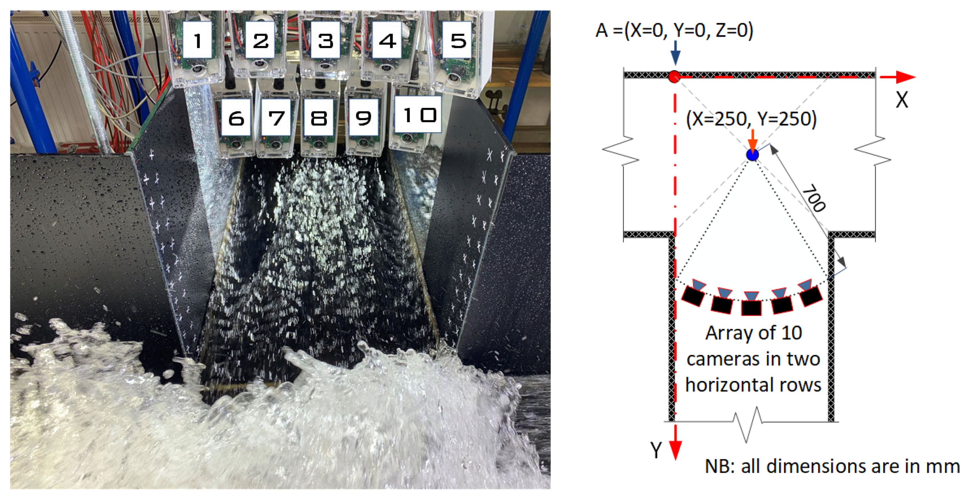
We used the following three-dimensional coordinate system for all measurements and analyses. The longitudinal axis originated at the beginning of the junction, the transverse axis originated at the left bank edge of the main channel, and the vertical axis extended from the bottom of the channel (Figure 1, right).

2.2. Selection of Hydraulic Parameters

A single set of operating parameters was selected for analysis. The hydraulic parameters of the supercritical inflows, both characterised by high Froude and Reynolds numbers, for the selected scenario, are listed in

Table 1. Set of operating hydraulic parameters for selected flow conditions.

Variable	Value
main flow height [m]	0.02
side flow height [m]	0.02
main flow rate [l/s]	32.7
side flow rate [l/s]	22.2
main flow Fr [−]	7
side flow Fr [−]	5
main flow Re [−]	6.5 × 104
side flow Re [−]	4.4 × 104
main flow height [m]	0.02
side flow height [m]	0.02

. A pronounced three-dimensional turbulent aerated flow develops at the junction, forming unsteady and non-homogeneous standing waves. A 3D structure of the free water surface is formed in the transversal and longitudinal directions. Turbulent flow is characterised by high local velocity, steep surfaces, and large height differences. Turbulent structures on the water surface are non-linear and three-dimensional and include ridges, vortex swirls, waves, hairpin-like structures, turbulent bursts, and flying water droplets.

2.3. Photogrammetry Procedure

Laser scanning methods based on measuring the distance between the instrument and the observed object surface obtain information by applying relatively simple post-processing procedures [10]. Due to the rapidly changing free water surface of turbulent and highly aerated water flows, such as those considered in our study, post processing of the photogrammetric image dataset requires several steps that are not fully automated. The procedure for the acquisition and post processing of the photogrammetric image data consisted of the following steps:

• Setting up the experiment, including mounting and arranging the array of cameras and LED illumination, and performing reference and tie points measurements using a precise terrestrial survey;
• Acquisition of image datasets at different times;
• Post processing of the image datasets and creating point clouds.

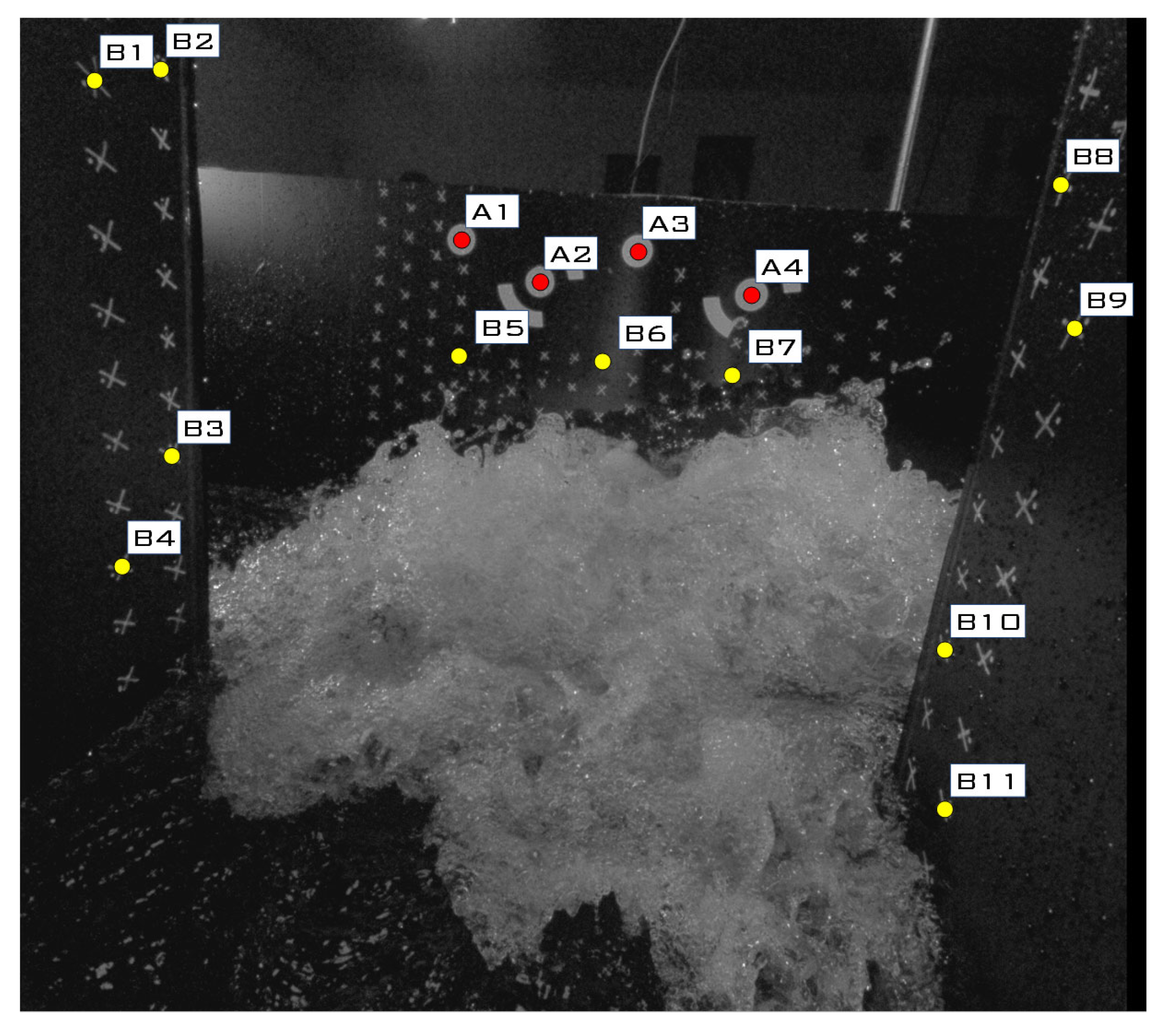
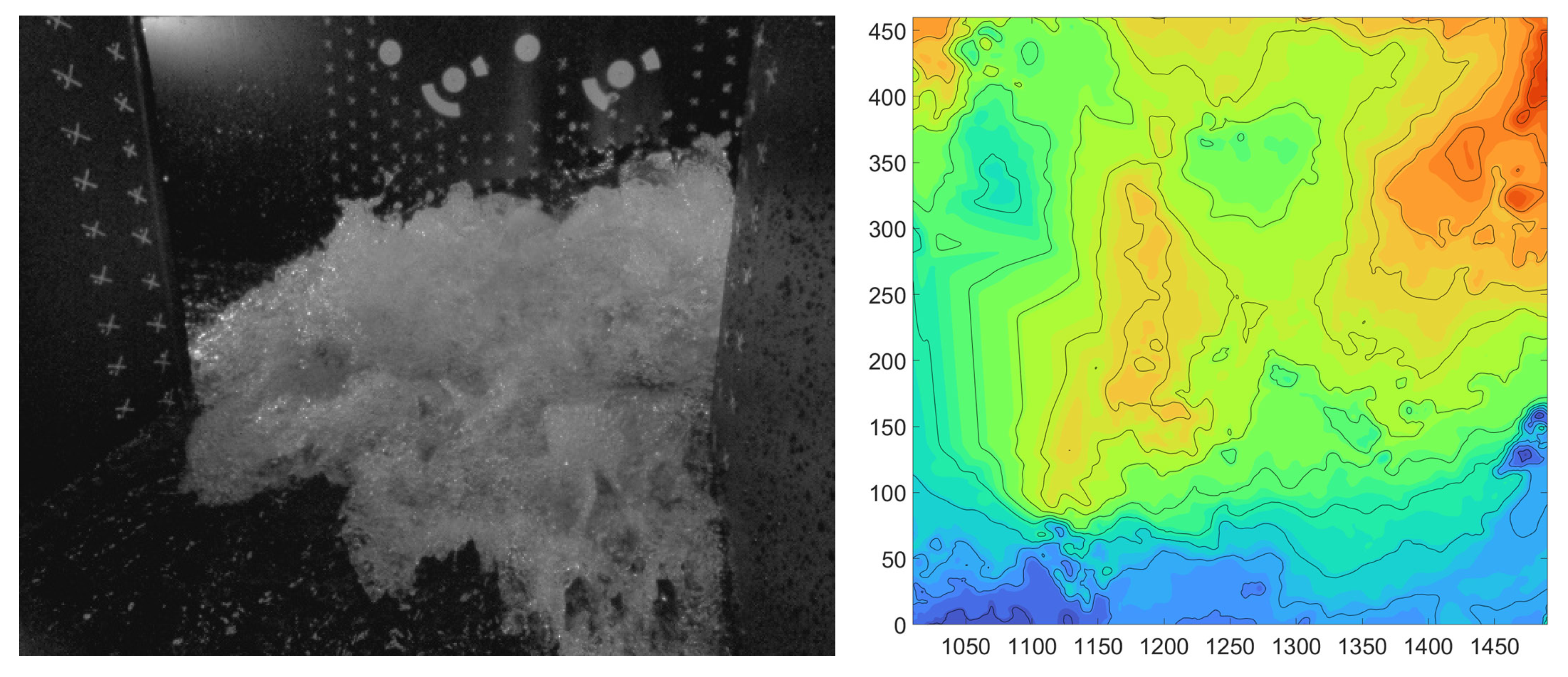
To achieve better contrast and minimise unwanted reflections in the acquired images, a matte black foil was applied to the channel walls throughout the acquisition area (Figure 2).

As reference points, the 4 markers in the form of circular patterns A1–A4 were attached to the black matte foil, while 11 reference points (B1–B11) were additionally selected among the tie points (Figure 2, white crosses).

The measurement station was equipped with 10 cameras of the type VEYE CS-MIPI-SC132 [36], as shown in Figure 3. The cameras have a resolution of 1.3 MP with a monochromatic sensor (image size 1/4″ with 1080 H × 1280 V) with a global shutter, multi-camera synchronisation option, and M12 × P0.5 lens mount [37]. The lens used was YT3.5-2M with a viewing angle of 97° (focal length 2 mm), 0.6% optical distortion, and an aperture of 3.5. All cameras were arranged in the side channel. A fixed shutter speed of 100 µs was maintained on all cameras for all experiments. Exposure, gain, shutter, and other image settings were manually adjusted and were the same and constant for all cameras. The optimal positioning of the cameras was determined to ensure sufficient longitudinal and transverse fields of view and their overlapping while maintaining the best possible image resolution. The precise positioning, uniform reference system, and stability of the cameras throughout the recording period were ensured by mounting them on an external frame structure that was not attached to the channel structure. The cameras were arranged in two horizontal rows, with the sensors’ centrelines positioned at heights of 350 and 550 mm above the channel bottom. In Figure 3 (right), a top view of the experimental setup is presented. The precise coordinates of each camera were determined using the SfM technique, relying on the coordinates of reference points measured during the precise terrestrial survey detailed in Section 2.4.

All cameras were triggered by an external trigger signal. The hardware triggering option was chosen to ensure sub-microsecond synchronisation. Accurate synchronisation of image acquisition was required due to the rapidly changing free water surface. The trigger signal was provided by the Raspberry Pi 4 microprocessor. Communication between the camera module and the microprocessor was via an Inter-Integrated Circuit IIC data transmission bus and a 15-pin FPC connector. Images were temporarily stored on the microprocessor and later transferred to the laptop computer via a Wi-Fi connection for further analysis. The open-source library was used for communication, camera parameter setting, and acquisition so that a single set of 10 synchronised images was acquired per acquisition. The procedure was repeated by the operator to acquire the desired number of image sets.

The field of view was illuminated with diffuse light from multiple LED lights installed at different positions relative to the imaging region of interest to ensure good visibility of features on the free water surface regardless of the viewing angle. Chip-on-load LED panels covering an area of 0.5 m × 0.5 m illuminated the confluence area from above, while additional LED lights (CREE XM-L2 type with collimating lens) were installed on both sides of the main channel (i.e., upstream and downstream) and in the side channel toward the downstream direction. To ensure spatially uniform illumination intensity throughout the area of interest, the LED panels and lights were carefully positioned and their output was adjusted by limiting the current to each light. To ensure flicker-free and continuous illumination, a high-quality DC power supply was used to power the lighting.

Knowing the exact position of the reference points was crucial for calculating the exterior orientation of the images and determining the position of the object in the local coordinate system, which was identical to the laser scanner coordinate system. To accurately determine the coordinates of all reference points in the local coordinate system, a precise terrestrial survey was performed using an electronic Total Station Leica TS30 (0.5″ angular accuracy and EDM accuracy 0.6 mm + 1 ppm) and prisms.

Due to the complex hydraulic phenomena and the interaction between water and light, such as reflection and refraction, obtaining a high point cloud density through photogrammetric image post processing requires a significantly larger number of reference points within the area of interest than measurements involving solid objects. When using multi-image methods to determine 3D coordinates, a well-distributed spatial arrangement of reference points can enhance the grid geometry, and thus the results of the SfM method [38,39,40].

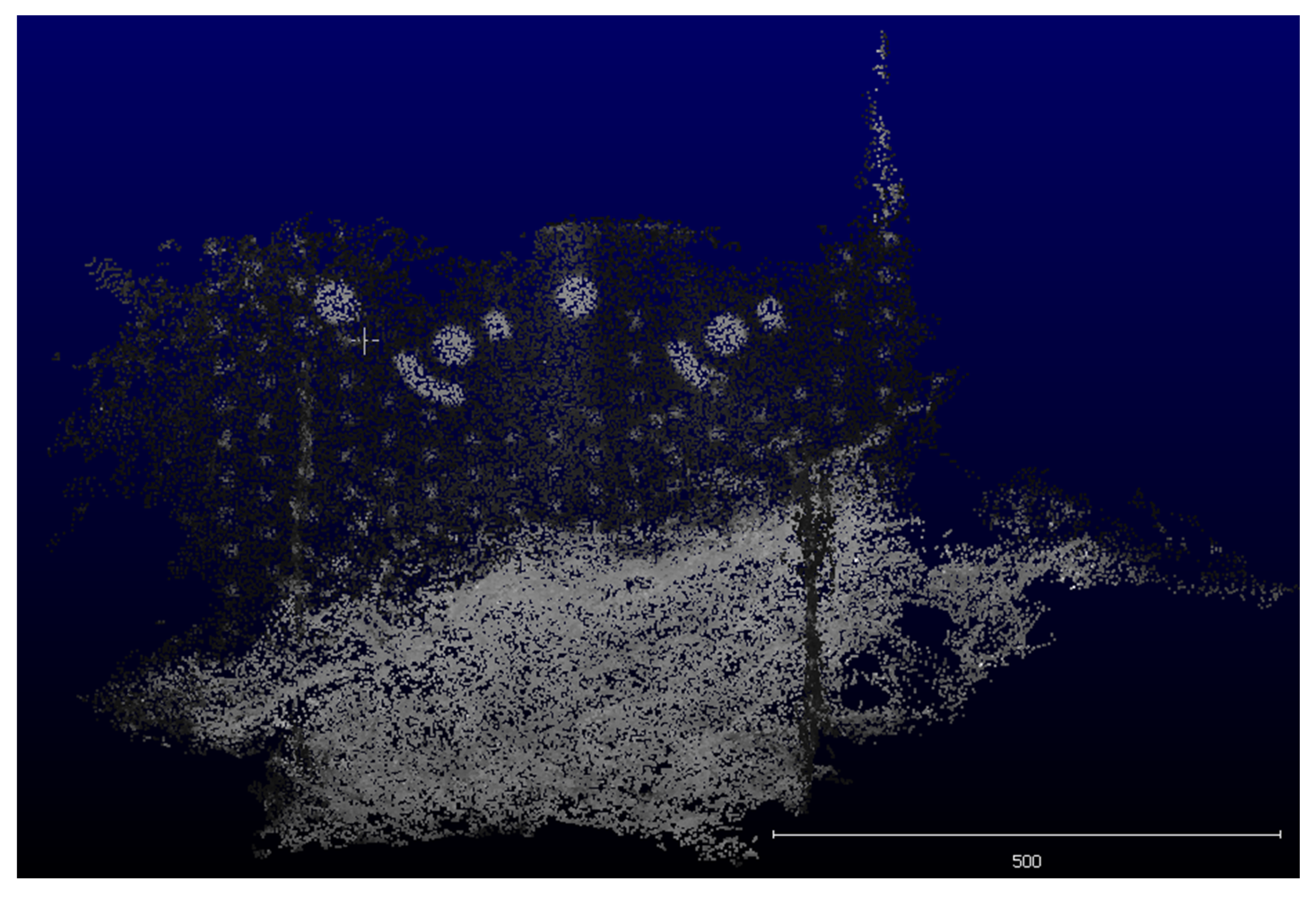
Post processing of the images and conversion to raw point clouds were performed using Agisoft’s Metashape software package (version 2.0.0), while further processing of the point clouds was carried out in CloudCompare (version 2.12.4), a robust 3D point cloud processing software known for its advanced capabilities. The Metashape software is based on the SfM method of photogrammetry, which was developed in the 1990s and relies on computer vision techniques. It is particularly well suited for multi-image photogrammetry applications. By combining SfM with MVS, the Metashape software package enables the generation of a point cloud representing the acquired surface from multiple overlapping images, while simultaneously calculating the exterior and interior orientation parameters of these images within a desired coordinate system (Figure 4).

The SfM method utilizes automatic image-matching algorithms to identify corresponding feature points in multiple images. These matched feature points are then used to compute the exterior and interior orientation parameters of the images as well as a low-density surface point cloud. To accomplish this, the coordinates of the previously identified and measured reference points were included in the calculations for the determination of the exterior and interior orientation of the images and the generation of a low-density point cloud in the reference coordinate system. The accuracy of the SfM calculations was verified by comparing the results to control points measured using precise terrestrial survey methods.

In the process of densifying the low-density point cloud, the MVS image-matching method is described in previous research publications [26,41,42]. This method helps to increase the point cloud density and provides a more detailed representation of the captured surface.

2.4. Precise Terrestrial Survey of the Reference Points

When the reference points were surveyed, various parameters were recorded, including horizontal angles, vertical angles, and slope distances. These measurements were essential for the accurate determination of the horizontal and vertical positions of the geodetic points in three-dimensional space. The unique combination of these parameters enabled the precise calculation of a point’s 3D position.

At each point, horizontal angles were measured using the method of angle sets (5 sets), while vertical angles and slope distances were measured in five repetitions in both faces. To ensure a high degree of accuracy, measurements of meteorological parameters were made simultaneously. These meteorological measurements played a crucial role in post processing, as they allowed for the calculation of corrections to the survey parameters [43].

The measurements were performed using a high-precision Leica TS30 Electronic Total Station, adhering to the specifications provided by the manufacturer, Leica Geosystem. The instrument specifications were according to σISO-17123-3 (hz, v) 0.5″ for horizontal and vertical angles and σISO-17123-4: 0.6 mm; 1.0 ppm for distances [44].

In addition to the electronic Total Station, other measuring instruments were used. These included three Leica GPH1P single precision reflectors (with a prism constant of 0), three Leica GZR3 rotating carriers with optical plummet precision reflector holders, a Meteo Station HM30 for meteorological measurements, and three tripods.

All data processing for the reference point measurements and determination of the local coordinate system were performed using our custom software algorithm. This algorithm was developed in MATLAB, taking into account the fundamental principles of the discipline. The tool has been extensively utilised and validated in previous survey projects, as documented in other publications [43].

The software algorithm includes several functionalities that ensure comprehensive data analysis. It checks the completeness of angle sets, calculates the arithmetic mean of angle sets, evaluates accuracy, determines approximate coordinates, reduces all measured distances to the surface ratio, and adjusts the results using the least squares method. These functions allow for robust processing and analysis of the measured data.

Based on the results of the fitting, it was determined that the maximum position error for a point is 0.3 mm, while the maximum height error is 0.45 mm. As expected, the accuracy of the height measurements is slightly lower compared to the position measurements.

By using our software algorithm and associated data processing functions, we have obtained accurate and reliable results in various surveying applications.

2.5. LIDAR Reference Measurements

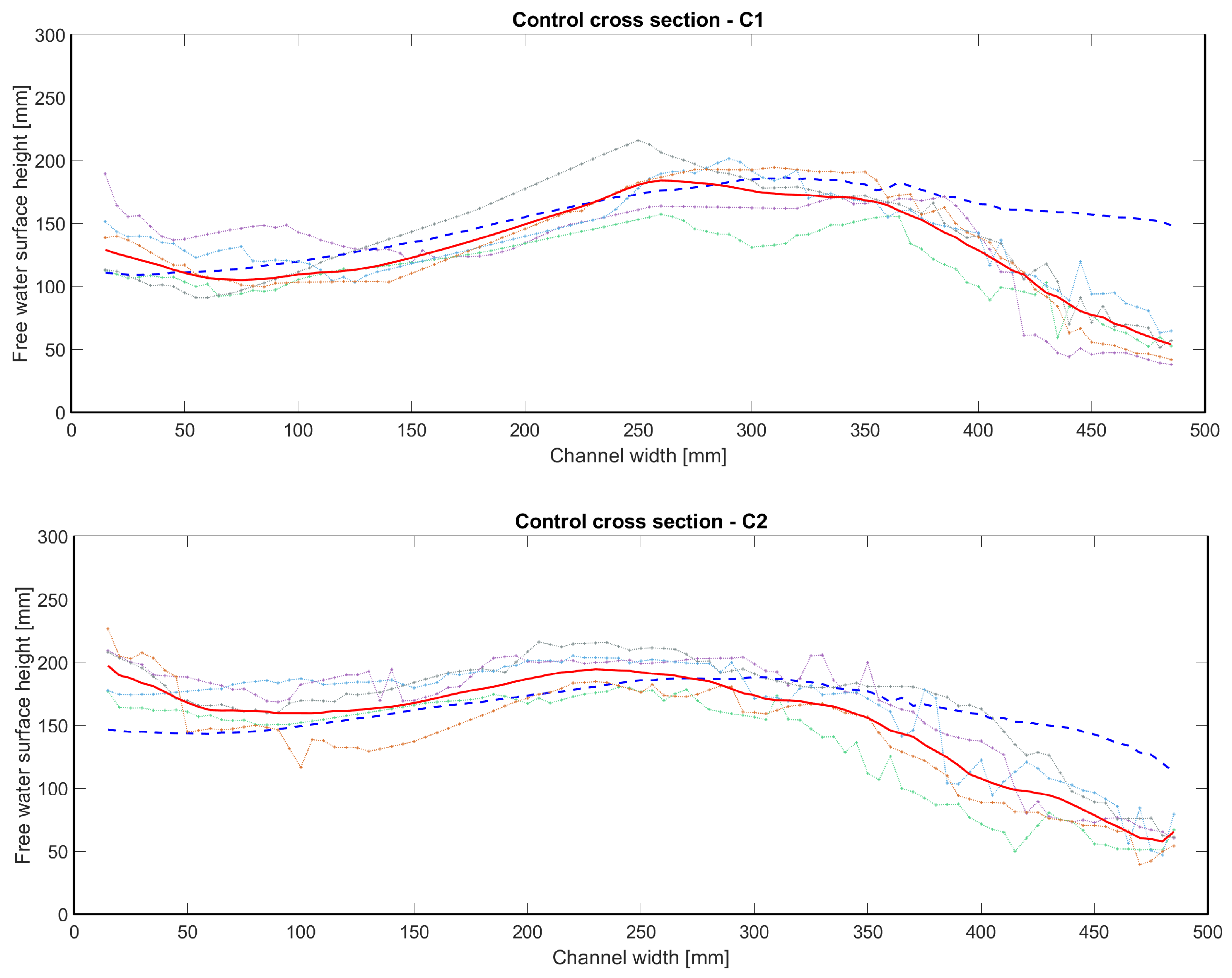
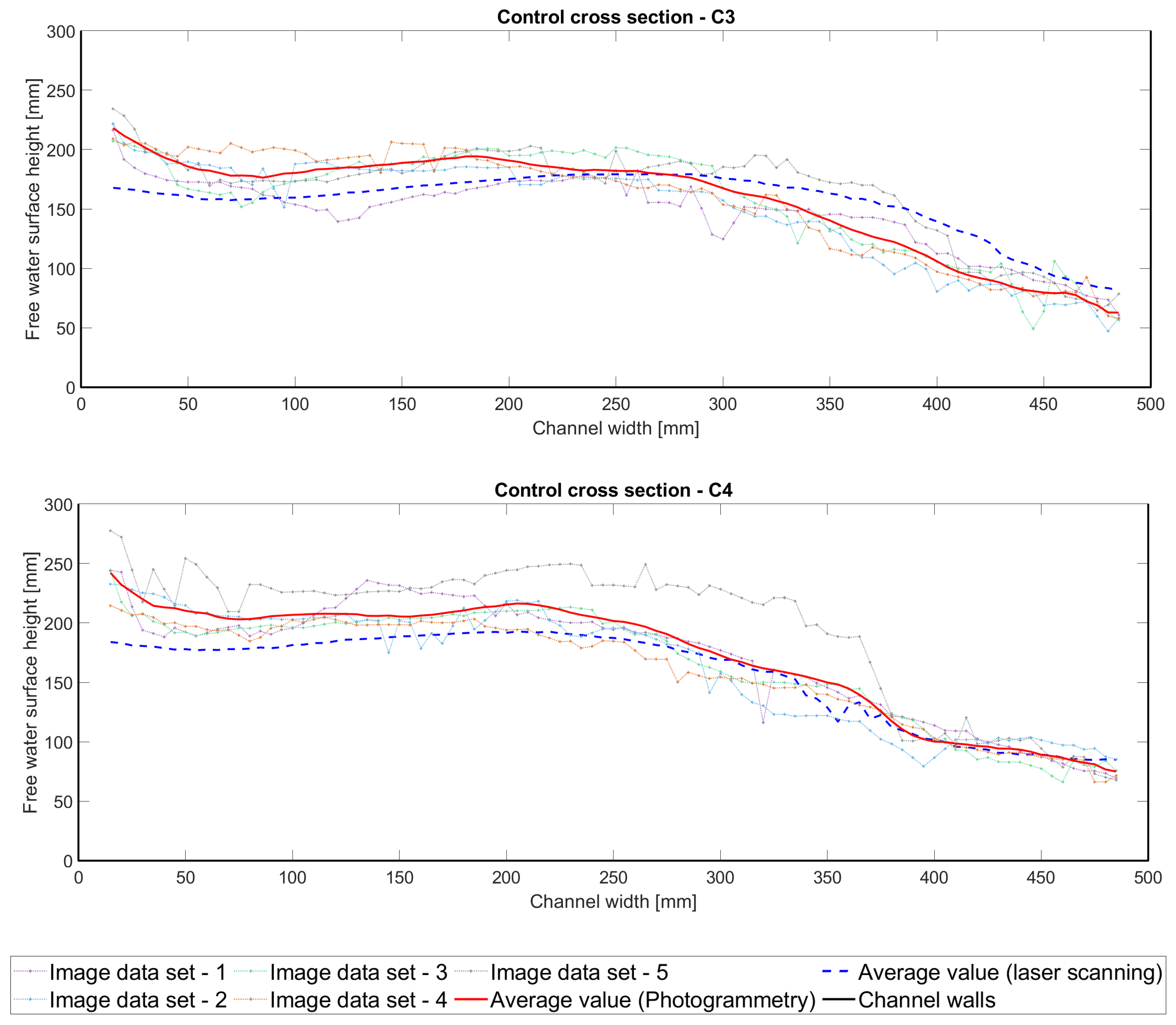
Reference profiling in specific cross sections was performed using a 2D laser scanner, which has demonstrated its robustness and effectiveness in acquiring the free water surface of turbulent aerated flows [10,45]. For comparison with photogrammetry, laser scanning measurements were made in four cross sections labelled C1 through C4, as shown by the blue lines in Figure 1, right.

For these measurements, we utilised the industrial laser scanner SICK LMS400 [46], which provides high temporal and spatial resolution along a scan line. The instrument operates at a visible red-light wavelength (λ = 650 nm) and was configured with a line scan frequency of 270 Hz and an angular resolution of 0.2°. The systematic measurement uncertainty and statistical measurement uncertainty of the instrument are ±4 mm and ±3 mm, respectively. The beam diameter is 1 mm. Each scan line consists of 350 measurement points within an angular range of 70°. A total of 6000 scan lines, and thus 2,100,000 points in the entire point cloud of each cross section, were used to reconstruct the average transverse profile of the free water surface. The laser scanner was placed at an elevation of 1150 mm above the channel bottom. Given the pronounced spatial non-uniformity in the free water surface profile and the objective of enhancing measurement precision, each profile was scanned from two distinct laser scanner positions along the transverse axis of the main channel, specifically at Y = 125 mm and Y = 375 mm. Detailed information on the post-processing techniques applied to the data from laser scanning can be found in previously published articles [10,14], which provide a comprehensive description of the methods used.

3. Results

The results section is divided into two parts. The first part presents the reconstruction of the free water surface using photogrammetry datasets, while the second part focuses on result verification through laser scanner measurements.

3.1. Reconstruction of the Free Water Surface Based on Photogrammetry Datasets

Following the post-processing steps detailed in Section 2.3, we created a raw point cloud from the acquired images. The point cloud was carefully positioned in the local coordinate system, as shown in Figure 1. To ensure accurate reconstruction of the free water surface, we filtered out points that represented non-water objects, such as walls or the bottom, as shown in Figure 5 (top).

Next, the unevenly distributed point cloud was rasterised. For this purpose, a raster grid with a resolution of 5 mm × 5 mm was chosen. Each node within the raster grid was assigned a vertical Z coordinate by a simple linear interpolation process. The same coordinate system was used before the rasterisation. The resulting rasterised point cloud is shown in Figure 5 (bottom).

Figure 5 shows a blind spot (x = 1000, y = 300) for which the photogrammetry method could not provide points. This particular area was not accessible to the cameras due to their positioning in the side channel and the height of the standing wave ridge. Additional cameras in the main channel would be required to effectively cover this area.

Reconstructing the free water surface using photogrammetry allows us to capture spatial variations in the topography of the water surface. By capturing a series of consecutive image sets at selected time intervals, we can effectively observe and analyse the temporal changes in the topography of the free water surface.

Figure 6 shows the corresponding images acquired by camera 7 (left), and the computed topography maps (right). It is important to note that the water in the main channel flows from left to right, while the inflow from the side channel is from below. Due to the imaging system used in this experiment, only a single image was captured per camera at any given time. This was because each microprocessor stored images locally for camera synchronisation, which later had to be sent to the main computer, and only then could the next synchronised set of images be captured. Therefore, the images in Figure 6 were taken at irregular intervals between shots. Nevertheless, the topography maps can be used to show the elevation differences of the free water surface of the junction flow.

The comparison (Figure 6) of camera images (left) and photogrammetric reconstruction (right) shows that the photogrammetric method reconstructs the standing waves very well. This is also true for the vertical (Z) direction, even in areas with significant variations in water height. This is in contrast to previous studies by Jašarević et al. [35], in which a much smaller number of cameras was used. An insufficient number of cameras in their study resulted in limited depth perception and consequently, an underestimation of the height of the free water surface. The results presented here demonstrate the importance of having a sufficient number of cameras for accurate water surface measurements in similar studies.

Consistent with the inherent nature of the hydraulic phenomenon itself, the overall shape of the reconstructed standing wave, as shown in Figure 6, remained relatively stable throughout the measurements. The maximum height of the wave, about 320 mm, remained relatively constant, while variations in the position and height of smaller and less significant local peaks were observed. We found that there is a blind spot at about (x = 1000, y = 300) in all four raw point clouds.

In the following section, we make a comprehensive comparison between the photogrammetry results and those of the LIDAR measurements. This analysis aims to highlight the strengths and limitations of each method and provide valuable insight into their respective effectiveness in capturing hydraulic phenomena.

3.2. Verification of Photogrammetry Data Using LIDAR Measurements

In this study, laser scanning, as a proven method for measuring turbulent, aerated free water surface flows, was used as a reference measurement method to verify the accuracy of the photogrammetric method. The laser scanning device allows for the comparison of profiles of the free water surface with those obtained by photogrammetry in selected cross sections. To enable the comparison with the photogrammetric method, we calculated average LIDAR profiles of the free water surface in control cross sections (C1 to C4 in Figure 1, right). The average profiles were calculated from 6000 consecutive scan lines acquired with a LIDAR scanner at a frequency of 270 Hz and an angular resolution of 0.2°.

In contrast to laser scanning, photogrammetry provided comprehensive coverage of the free water surface over the entire field of view of the synchronised cameras during im-age acquisition. Since the points in the raw photogrammetry point cloud were distributed along the cross sections where LIDAR measurements were taken, the profiles of the free water surface were extracted from the rasterised photogrammetry point cloud with a resolution of 5 mm × 5 mm for comparison.

Figure 7 shows the free water surface profiles for selected control cross sections C1 to C4. The free water surface profiles are shown for the individual photogrammetry image datasets, average profiles from all photogrammetry image datasets (solid, red), and average profiles from laser scanning (dashed, blue). The comparison allows for an analysis of the similarities and differences between the laser scanning and photogrammetry measurements.

The images of the measuring cameras (Figure 1 (left), Figure 2, Figure 3, and Figure 6) show high flow dynamics and turbulence in the entire measuring area. Nevertheless, the measurement results for cross sections C1–C4 show good agreement between the profiles of the free water surface obtained with the laser scanner and the averaged photogrammetry profile for a large part of the profile. Except in the area where side inflow meets water flow in the main channel and aerated standing waves begin to form (right side of profiles C1 and C2), laser scanning results in a higher free water surface. This is not consistent with the results of previous studies on laser scanning measurements. Water heights measured with laser scanners are often underestimated because they are reflected from bubbles in deeper water layers or from multiple successive laser beam reflections within the aerated portion of the surface. Here, we find that reflections from flying droplets are more pronounced. The effect of reflections from flying droplets could not be completely avoided even by filtering the point cloud with a remission threshold. Indeed, due to light scattering and energy dissipation on the path of the beam through the water, the measurements resulted in significantly lower remission values of the returned signals reflected from immersed air bubbles [14].

As discussed by Rak et al. [10], it is important to consider the behaviour of the laser scanning signal, which may be reflected multiple times by droplets and air bubbles before returning to the instrument. In addition, the speed of light in water is approximately 25% slower than in air. Both of these factors contribute to a longer time of flight and consequently, an overestimation of the measured distance, resulting in the determination of lower water height. On the right side of profiles C1 and C2 in the intervals from about 400 mm to 500 mm, higher water levels measured by the laser scanner can be attributed to turbulent vortices, air entrainment, intense spraying, and larger droplets that occur in the region where the flows in the main and side channels meet. Based on our understanding of these phenomena and analysis of the images, it can be concluded that photogrammetry provides more reliable results in this particular area.

A more significant deviation between the profiles of the free water surface, as averaged by laser scanning and photogrammetry, is also noticeable in the area near the opposite wall, specifically within the range of 0 mm to about 50 mm. Within this region, the intense flow dynamics, turbulence, and interaction with the wall create unsteady flow structures resulting in greater fluctuations in the free water surface (best shown in Figure 1). However, except for these two regions mentioned above, both methods show good agreement over most of the cross sections, with variations within ±20 mm. Figure 8 illustrates the degree of agreement and range of deviations between the averaged profiles of the free water surface obtained by laser scanning and photogrammetry. Despite the general underestimation of water levels due to the above factors, the laser scanning measurements with the applied correction based on remission values agree well with the photogrammetry results.

The profiles of free water surface in individual cross sections obtained from each photogrammetry image dataset (i.e., in the selected time) allow for the evaluation of free water surface variations around an average value. The average fluctuations in all analysed cross sections were within ±25 mm, while the maximum fluctuations can reach values up to ±60 mm. For profiles C2 and C3, Figure 9 shows the variations in free water profiles obtained from the individual photogrammetry image datasets compared to the averaged profile based on all five image datasets. Similar variations in the dynamics of the free water surface were also found when analysing the image sequence acquired with a high-speed camera at individual points and the laser scanning point cloud filtered based on the remission of the returned signals [14].

4. Discussion

Accurate measurements of free water surface flows play a pivotal role in a wide range of engineering applications, encompassing civil, chemical, environmental, mechanical, mining, and nuclear engineering. In turbulent free surface flows, the deformation of the surface leads to the entrainment of air bubbles. When the turbulent shear stress exceeds the surface tension stress that opposes interfacial breakup, air bubble entrainment becomes possible. Characteristics of aerated flows have been studied experimentally, numerically, and theoretically. In all these fields, free water surface measurements are essential for gaining insight into and understanding the complexities of turbulent and aerated flows. In comparison to the already proven measurement techniques, particularly LIDAR, the limitations of the proposed method encountered to date and the challenges that can be expected in the next steps of applying the method both in the laboratory and in the field, are discussed in detail.

Over recent years, laser scanning has increasingly replaced conventional methods for measurements of hydraulic phenomena where turbulent, vortexing, and distinctively 3D flow with large free water surface fluctuation amplitudes occur [9,10,12,15,16,17,45]. Two-dimensional laser scanner measurements with high temporal resolution usually allow for measurements in a single cross-sectional profile. This restricts the reconstruction of objects to a certain number of consecutive scan lines performed by the physical movement of the 2D laser scanner. As a result of the movement, the temporal resolution of these 3D scans is low. It is also important to note that the interaction between the laser beam and the aerated water surface is unique and results in a relatively low reflection rate of about 5% of the laser signals detected by the photodetector. This is in contrast to solid surfaces, where the reflection rate is typically close to 100%. Nevertheless, relevant publications show that the performance of laser scanners in these experimental setups is still comparable to the results of average surface measurements using conventional methods within the limits of measurement uncertainty [9,12,13,14,45], while significantly exceeding them in capturing the temporal dynamics of the phenomenon.

In contrast, photogrammetry captures the entire field of view at each successive time, allowing for a full 3D object reconstruction with high spatial resolution, while the temporal resolution is similar to 2D laser scanners. The temporal resolution of a photogrammetric acquisition depends on the characteristics of the cameras, the possible use of microprocessors for temporal storage of the images, and the data transfer protocols from microprocessors or cameras to the main computer. In addition, photogrammetric methods require much more complex post-processing procedures compared to laser scanners.

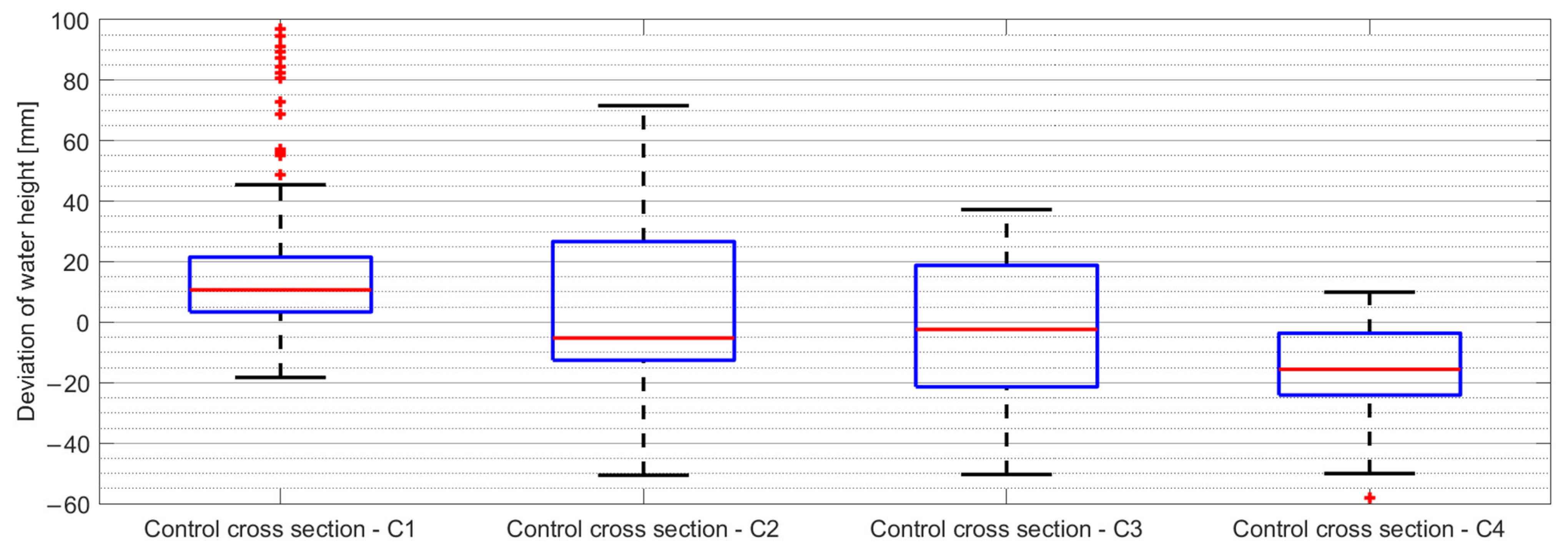
In contrast to laser scanners, photogrammetry is not based on the principle of distance measurement. By comparing the characteristics of the point cloud data produced by each method, we estimate the uncertainty of laser scanner measurements for solid objects (about ±3 mm) and the estimated error for measurements in aerated waters in the range of ±5–10 mm [14]. In photogrammetry, accuracy depends on a variety of factors, including the precision of the model produced, the accuracy of reference points measured, image quality, synchronisation error, the algorithm used to determine the tie points, point cloud generation, rasterisation, etc. In this work, the uncertainty of the point cloud after rasterisation was estimated to be about ±5 mm. Considering the similar error magnitude in both methods, it can be concluded that the methods are comparable in terms of accuracy and laser scanning is suitable for verifying the accuracy of a photogrammetric point cloud.

From the standpoint of capturing the entire visible area of the cameras and providing a more accurate representation of the topography of the free water surface, photogrammetry proved to be the better method. It provides a better representation of the flow conditions in the experiment. On the other hand, when reconstructing the water level based on cross sections from LIDAR measurements, the influence of interpolation and smoothing between these sections is greater.

However, there are also some potential drawbacks in using photogrammetry to reconstruct the free water surface. The water surface is specular and transparent, leading to very complex reflection mechanisms. This complexity is particularly pronounced when interacting with a turbulent and non-homogeneous aerated free water surface characterised by substantial vertical fluctuations and an abundance of flying droplets and submerged trapped air bubbles. The occurrence of total internal reflections (especially at the bubble and droplet surfaces) at high incident angles of the incident light, combined with reflections at the liquid mass, can cause neighbouring cameras to capture very different images of local free surface segments. To reduce this phenomenon to the greatest extent possible, diffuse light from many different angles was used in our experimental setup. Since the effect of complex light reflection mechanisms on the measurement uncertainty of the photogrammetric method used is beyond the scope of this article, its evaluation on a functional level is discussed by comparing it with the results from laser scanning. Given that the proposed approach is currently still in the development phase and ensuring adequate illumination for field measurements poses challenges, its current applicability is restricted to laboratory experiments and the physical modelling of complex hydraulic phenomena. Nevertheless, achieving precise and accurate measurements is critical to understanding these phenomena and effectively designing hydraulic structures. Since laboratory-based hydraulic research holds significant importance for the design of hydraulic structures, this approach could already find practical application.

5. Conclusions

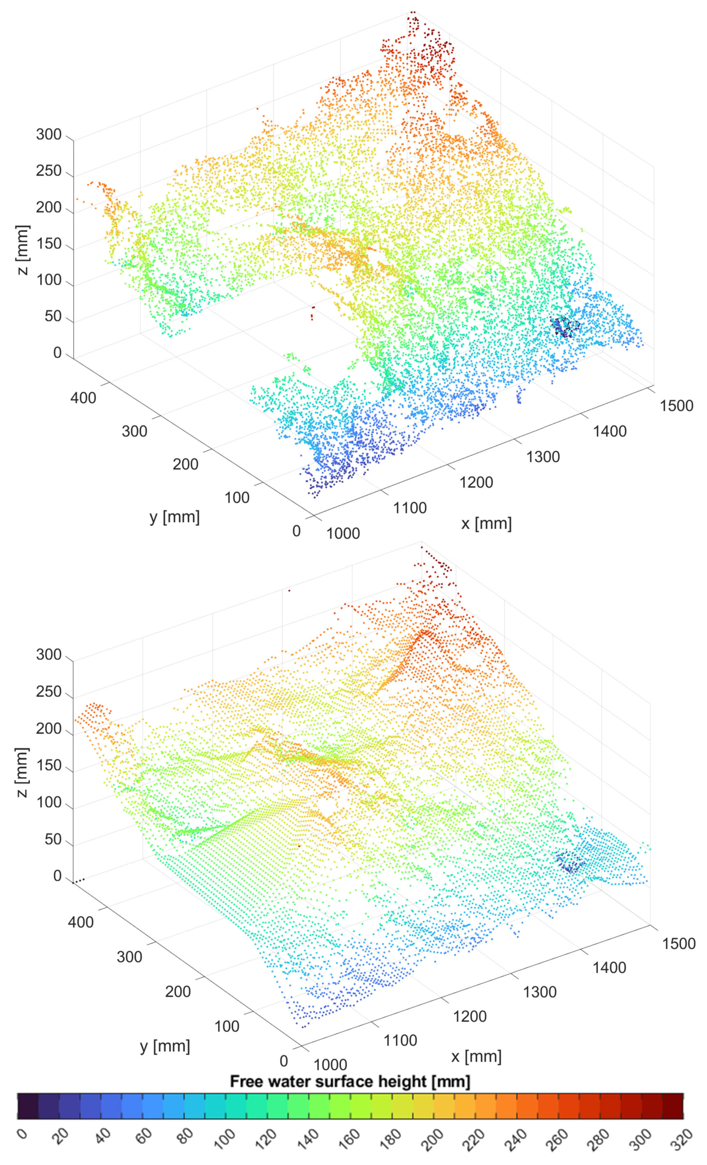
In the expected future challenges in hydraulic engineering, the most important re-search topics are likely to be in the area of complex hydraulic phenomena associated with high-velocity flows and, in particular, air-flow properties. Accurate measurements of free water surface flows are crucial for both hydraulic and mechanical engineering applications. They are essential for gaining insight into and understanding complex, turbulent, and aerated flows. In this paper, an experimental setup and a photogrammetry-based method for measuring the topography of the aerated free water surface were developed. A turbulent and highly aerated confluence flow forming standing waves was chosen as a case study. The combination of SfM and MVS methods of photogrammetry reconstruction methods implemented in professional software packages provided the best results. In this way, we were able to produce accurate topography maps of highly complex 3D water structures as used in the standing wave experiment.

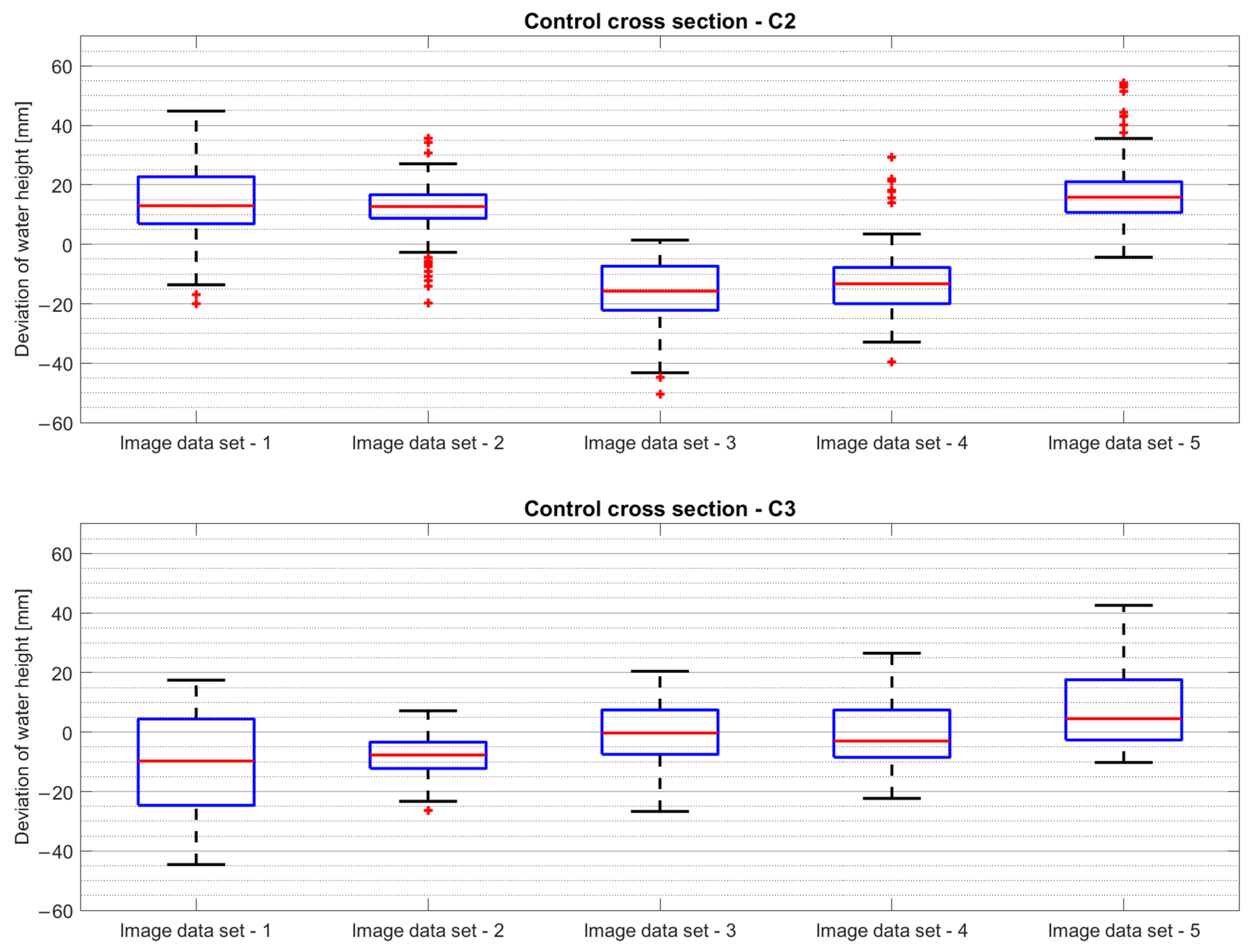
For the above case, we show a good agreement between photogrammetry and the now well-established laser scanning method for a selection of four free water surface profiles in the middle of the junction. To achieve this, sufficient camera coverage and overlap of the flow phenomenon of interest is required, combined with completely uniform and continuous illumination. Validation with LIDAR data revealed deviations within ±20 mm. A significant distinction lies in the fact that photogrammetry enables the reconstruction of the free water surface topography within the entire field of view of the cameras from a single image dataset.

Free water surface reconstruction is a valuable tool for visual and in-depth analysis of the spatial variations and dynamic fluctuations that occur in the topography of the free water surface. By capturing a series of consecutive images at specific time intervals, the method is interesting for observation and visualisation, analysis, investigation, and comprehensive understanding of the topography of the free water surface.

It is also important to recognise the potential drawbacks associated with using photogrammetry to reconstruct the free water surface. The aerated free water surface is both specular and transparent, resulting in extremely complex reflectance sequences. Total reflections can occur at high incident angles of the incident light, especially at the surfaces of bubbles and droplets. These reflections, in combination with reflections from the liquid mass, can cause even adjacent cameras to capture significantly different images of local free water surface segments. These large discrepancies can complicate the photogrammetric processing algorithm.

We can see the main potential for future developments and applications of the presented photogrammetric method in the use of synchronised high-speed camera arrays for high-resolution measurement of instantaneous flow topography, especially in unsteady or otherwise highly complex flows where laser ranging methods may perform poorly.