Mapping Agricultural Land in Afghanistan’s Opium Provinces Using a Generalised Deep Learning Model and Medium Resolution Satellite Imagery

Abstract

Understanding the relationship between land use and opium production is critical for monitoring the dynamics of poppy cultivation and developing an effective counter narcotics policy in Afghanistan. However, mapping agricultural land accurately and rapidly is challenging, as current methods require resource-intensive and time consuming manual image-interpretation. Deep convolutional neural nets have been shown to greatly reduce the manual effort in mapping agriculture from satellite imagery but require large amounts of densely labelled training data for model training. Here we develop a generalised model using past images and labels from different medium resolution satellite sensors for fully automatic agricultural land classification using the latest medium resolution satellite imagery. The model (FCN-8) is first trained on Disaster Monitoring Constellation (DMC) satellite images from 2007 to 2009. The effect of shape, texture and spectral features on model performance are investigated along with normalisation in order to standardise input medium resolution imagery from DMC, Landsat-5, Landsat-8, and Sentinel-2 for transfer learning between sensors and across years. Textural features make the highest contribution to overall accuracy (∼73%) while the effect of shape is minimal. The model accuracy on new images, with no additional training, is comparable to visual image interpretation (overall > 95%, user accuracy > 91%, producer accuracy > 85%, and frequency weighted intersection over union > 67%). The model is robust and was used to map agriculture from archive images (1990) and can be used in other areas with similar landscapes. The model can be updated by fine tuning using smaller, sparsely labelled datasets in the future. The generalised model was used to map the change in agricultural area in Helmand Province, showing the expansion of agricultural land into former desert areas. Training generalised deep learning models using data from both new and long-term EO programmes, with little or no requirement for fine tuning, is an exciting opportunity for automating image classification across datasets and through time that can improve our understanding of the environment.

1. Introduction

Afghanistan supplies more than 80% of the world’s opiates. Changes in Afghan opiate production have far-reaching consequences for trafficking activities and the flow of illicit money as well as for the high dependency users of heroin and opium. Understanding and monitoring opiate production in the country is therefore of great importance for the international community and the United Nations Office on Drugs and Crime (UNODC) conducts annual opium cultivation and production surveys [1].

The relationship between land use and poppy cultivation is critical for monitoring the dynamics of opium poppy cultivation, and thus for evaluating and developing effective counter narcotics policy to reduce opium production. In the main opium provinces of Afghanistan, the availability of agricultural land is strongly correlated to opium cultivation, making up-to-date and accurate information on agricultural land a requirement for efficient monitoring [2]. The land used for cultivating opium poppy can fluctuate strongly from year to year and is driven by many socio-economic and agro-economic factors, such as water and resource availability, land rotation and agricultural expansion [3,4]. For example, access to solar-powered pumps and fertilisers have enabled some poppy farmers to relocate to former desert areas, increasing the total area of land available for opium poppy cultivation in Helmand, one of the main cultivating Provinces, resulting in an unprecedented increase in opium cultivation in the 2010s [5].

Satellite imagery can be used to map agricultural land as it provides a synoptic view of the landscape that can be timed to coincide with the presence of crops. 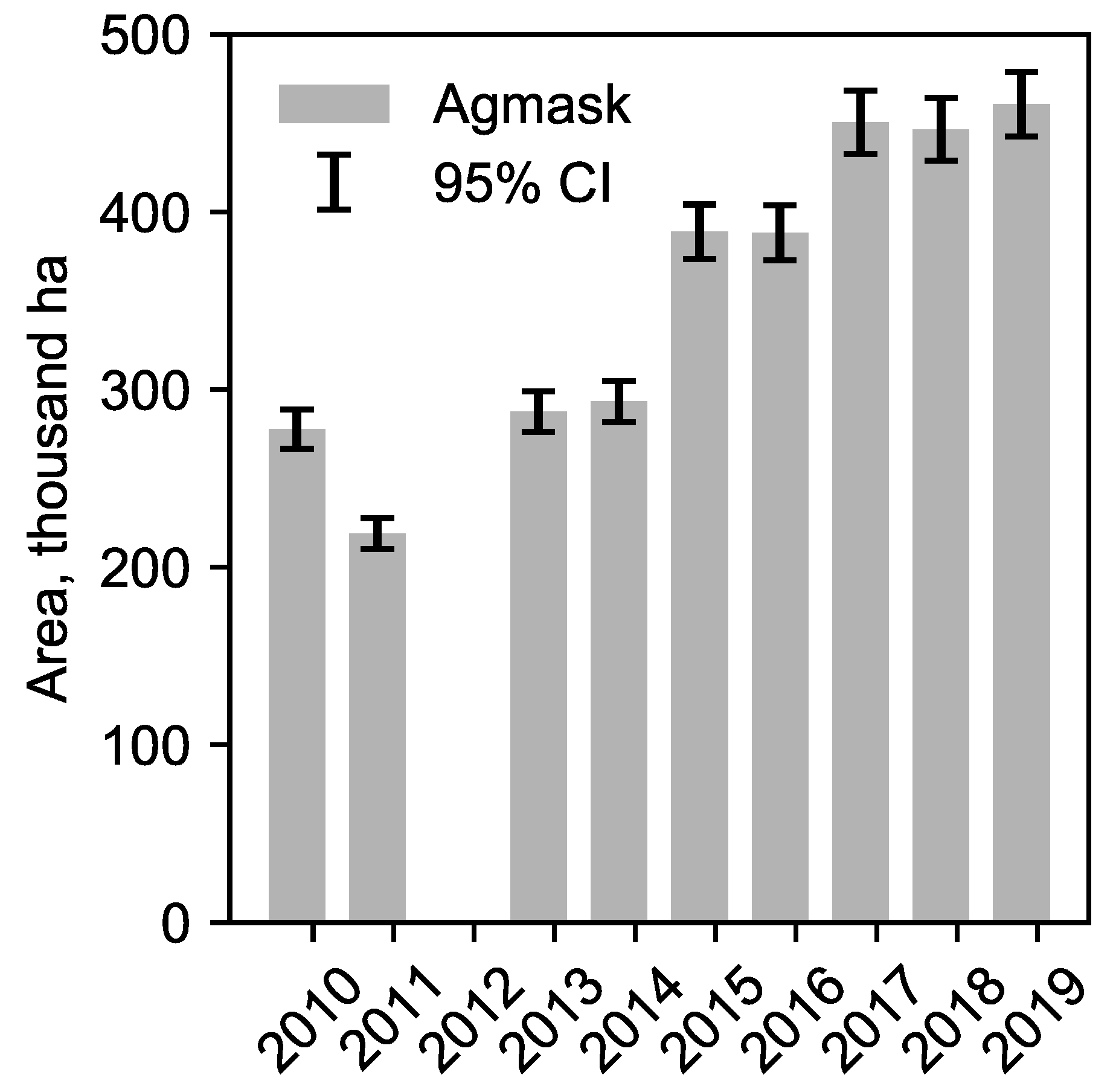The UNODC uses a combination of digital classification and visual image-interpretation of Landsat-8 Operational Land Imager (OLI) data, supplemented with Sentinel-2 and very-high resolution imagery (VHR), to create an agricultural mask, or agmask, that defines the sampling frame for their annual survey of opium production in Afghanistan [2]. This methodology is time consuming and resource intensive, making the creation of an annual map impractical. Instead a pragmatic approach of adding new areas of agriculture on an ad-hoc basis is taken, with each year’s agmask largely based on the previous year. This results in a conservative agmask, that tends to over-estimate the agricultural land that can used for opium poppy cultivation. While this avoids underestimation of opium poppy caused by the omission of potential land, it reduces the efficiency of the sample used for obtaining VHR satellite imagery, collected for estimating the area under opium poppy cultivation, and does not capture the inter-annual changes in agricultural land.

Recent work has shown the potential to produce accurate and timely agricultural land classification from satellite imagery using convolutional neural networks (CNNs) [6,7]. These deep learning models differ from conventional pixel- and object-based approaches in that they can be trained across multiple years of image data using transfer learning: where a pre-trained model is fine tuned using new labelled image data from a much smaller dataset than was used to train the original model. Ref. [6] found that transfer learning in Afghanistan’s Helmand Province between years required 75% less labelled data than models trained from scratch (no prior training), with improved overall accuracy (>94%).

An explanation for the improvement in model accuracy with fine tuning is that each image-specific dataset contains a subset of all possible observations, so as more data becomes available the model gets better at extrapolating, or generalising, to unknown instances as they are more likely to fall within the distribution of the training data [8]. The challenge is creating the large amounts of labelled data required to train the model to the required accuracy [9]. Utilising datasets that already exist would reduce the need for costly and time consuming image labelling and provide a broader set of training examples. However, these historical data are likely to be from a range of different sensors, some of which are no longer operating, and the resulting models would need to accurately classify image data from the latest Earth Observations (EO) programmes. The difficulty in leveraging historical data is the inherent radiometric and atmospheric differences between image acquisitions, which means, in general, different images require different analysis and models, especially for supervised classification [10].

In this paper, we investigate the characteristics of agricultural land in Afghanistan that span different image datasets and use this new knowledge to train a generalised deep learning model to classify new (or archive) images, without the need for any further training, to achieve fully automated mapping. The generalised model is used to map the evolution of agricultural land in Helmand Province, including hindcasting, on Landsat and Sentinel-2 data from 1999 to 2019. The ability of the model to generalise to other geographical areas is tested in Farah and Nangarhar Provinces with no additional training. The novelty in this work is the creation of a model trained using images and historical labelled data from different satellite sensors over time, which can be used to classify images from any medium resolution image.

2. Materials and Methods

A generalised model for agricultural land classification was developed using historical labelled image data at medium resolution (∼30 m). First, to optimise preprocessing of inputs for transfer learning, the contribution of shape, texture, and spectral image features to agricultural land classification were investigated, along with different approaches to standardising image pixel values. Second, we trained a CNN year-on-year with dense and sparse datasets between 2007 and 2017 for use as a generalised classifier of agricultural land from medium resolution images. This generalised model was then used to map the yearly changes in agricultural land in Helmand Province from 2017 to 2019, and in two other provinces, with no further training. The individual steps are detailed in the following subsections.

2.1. Study Area

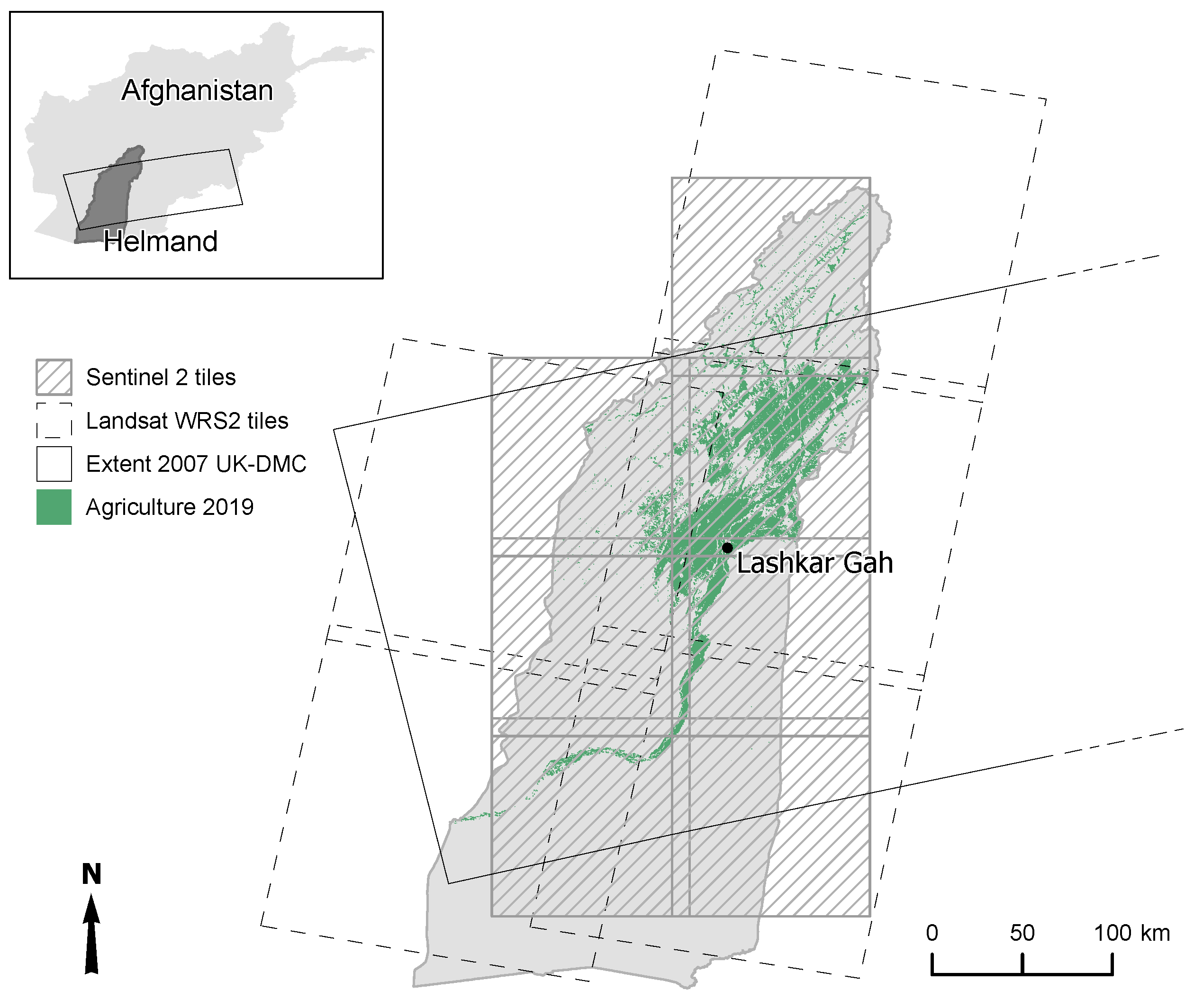
The study area is Helmand Province in the south of Afghanistan (Figure 1), which is the largest opium producing province in Afghanistan with an estimated 109,778 ha grown in 2021, accounting for 60% of national opium cultivation [11]. The majority of the Province is desert plain with the main area of cultivation in the Helmand river valley. There are areas of natural vegetation (needle leaved trees and shrubs) in the mountainous north of the Province. The agricultural landscape is dominated by irrigated crops of poppy and wheat but also includes fruit trees, vineyards, and rain-fed crops in lowland and highland areas [12]. Agriculture is reliant on snowpack melt to supply sufficient groundwater for irrigation, with water availability one of the main drivers for changes in agricultural area [4,13].

2.2. Model Training and Evaluation Datasets

Labels for training and evaluation of the models were created from existing maps of agricultural land for Helmand Province using a targeted training strategy [6]. Labelled datasets of active agricultural land and orthorectified Disaster Monitoring Constellation (DMC) images, with near-infrared (NIR, 0.76 to 0.90 µm), red (R, 0.63 to 0.69 µm), and green (G, 0.52 to 0.62 µm) bands at 32 m spatial resolution for 2007 and 2009 (

Table 1. Satellite images used for model development, transfer learning, and evaluation with central wavelengths for image sensor bands. The Images for the timing experiment are in italics.

Image Sensor	Image Date	Resolution (m)	Revisit Time	NIR, R, G (µm)
DMC	27 April 2007	32	Up to daily	0.83, 0.66, 0.57
	24 March 2007
	7 April 2008
	24 April 2008
	25 March 2008
	3 April 2009
	8 April 2009
Landsat-5	28 March 2009	30	16 days	0.83, 0.66, 0.56
	30 March 2009
	5 April 2009
Landsat-8	26 January 2015	30	16 days	0.87, 0.66, 0.56
	27 February 2015
	15 March 2015
	31 March 2015
	7 April 2015
	16 April 2015
	2 May 2015
	3 June 2015
	24 March 2016
	18 April 2016
	27 March 2017
	5 April 2017
Sentinel-2a	8 April 2017	10	10 days	0.84, 0.67, 0.56
	15 April 2017

) were taken from opium poppy cultivation surveys detailed in [3].

Input images from each year were split into individual image chips, or patches, using a non-overlapping 256 × 256 pixel grid. The chip size was chosen so samples would easily fit within memory on a NVIDIA Quadro K2200 graphics card during training. Chips containing vegetation not classified as agriculture in the agmasks were identified using a simple threshold of Normalised Difference Vegetation Index (NDVI) ($NIR-R/NIR+R$), calculated at the image level using the Otsu method [14]. All chips with no vegetation were discarded, as the majority of chips contain no agriculture and the background class is well represented in the remaining agricultural chips. The selected chips were then ordered according to proportion of agriculture and split into a 75% training and 25% validation set by drawing every fourth chip from the ordered set, resulting in 415 training samples and 137 validation samples for each year.

Agricultural masks for Helmand Province from 2015 to 2017 were obtained from the UNODC. These agmasks differ from the 2007 to 2009 data as they represent the potential agricultural area for that year, including any fallow areas, and define the area-frame for the UNODC’s annual opium survey [15]. Image datasets for the UNODC labels were selected for model development (2009 Landsat-5) and transfer learning (Landsat-5 & 8 and Sentinel-2a) from cloud-free scenes as close as possible to the peak in the first vegetation cycle [16] and paired with the agmasks (Table 1). Multiple images for each year were used because of differences in peak opium biomass (approximately 1–2 weeks) between the north and south of the province [3]. Landsat-5 and Landsat-8 OLI images were downloaded from the United States Geological Survey Earth Explorer as level-1A top-of-atmosphere reflectance and Sentinel-2a images from The Copernicus Open Access Hub. Bands for each image were then stacked into false colour near-infrared composites (FCC) to match the bands of the DMC. Samples for training and evaluation were selected using the same sampling strategy as the 2008 and 2009 DMC data.

Each sample comprised an image FCC chip and labels on the same pixel grid (i.e., one label per pixel). The sampling strategy was found to be efficient during training compared to using all the data or a purely random sample as the examples were drawn from a balanced sample containing a higher number of natural vegetation pixels—the main source of confusion.

2.3. Deep Fully-Convolutional Neural Network

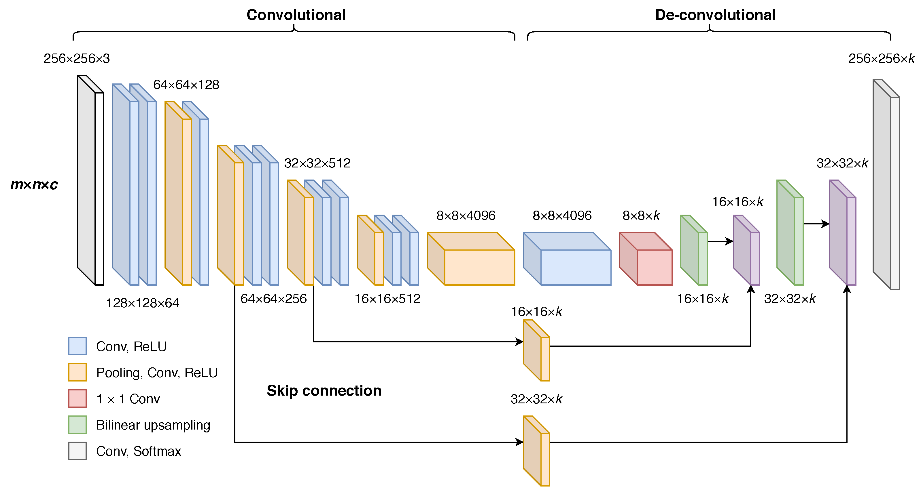
Fully-convolutional neural networks are a subset of deep learning models that are well suited for use with satellite imagery. Their main advantage is that inference takes place at the pixel level, without any flattening of the data, as input pixels are path-connected to the output classification [17]. In practice, this means that models can be trained and evaluated on images of different dimensions, with image size limited to the available memory on a Graphical Processing Unit (GPU), and the relationships between adjacent pixels are maintained.

Fully Convolutional Network 8 (FCN-8) of [17] was selected for this study because of its relative simplicity and the performance of U-Net type CNN architectures for semantic segmentation of satellite image data [18]. The network is built up of convolutional layers, where each layer can be though of as a kernel operation using filter weights k of shape $m\times n\times c$, with width m, height n and depth c. Starting with the input image, each subsequent layer with pixel vector $\mathbf{y}$, at location $i,j$, is computed from the previous layer ($\mathbf{x}$) by

$${\mathbf{y}}_{i,j}=f_{k,s}\left({\left\{{\mathbf{x}}_{si+\delta i,sj+\delta j}\right\}}_{0\le \delta i,\delta j<k}\right),$$

(1)

where f is a matrix multiplication and the offsets $0\le \delta i,\delta j<k$, along with the stride s, map the input spatial region, known as the receptive field. Pooling layers down-sample inputs to encode complex relationships between pixels, with an increasing number of features (dimension c) at the expense of spatial resolution ($m\times n$). The deeper layers are up-sampled back to the 2D dimensions of the input using de-convolutional layers. Information from preceding layers is fused with the up-sampled layers using skip connections that add finer spatial information to the dense output. Scoring takes place before fusing to reduce the depth of the layer to the number of output classes (Figure 2).

FCN-8 model code (available at https://github.com/dspix/deepjet (accessed on 2 August 2023)) written for TensorFlow [20] was used for all experiments within the open source Anaconda Python distribution [21]. Convolutional layer weights were randomly initialised and up-sampling layer weights initialised as bilinear filters as suggested in [17]. All models were trained on a NVIDIA Quadro K2200 GPU. The cross entropy loss between the model predictions and labels was summed across the spatial dimensions at each training step and gradients optimised using Adam [22] with a learning rate of 10${}^{-4}$. To avoid over-fitting a 50% dropout rate was applied to layers 6 and 7 and model training was stopped after 50 epochs. This was found by experiment to be long enough for the training loss to stabilise without an increase in the validation loss, which would indicate over-fitting of the model.

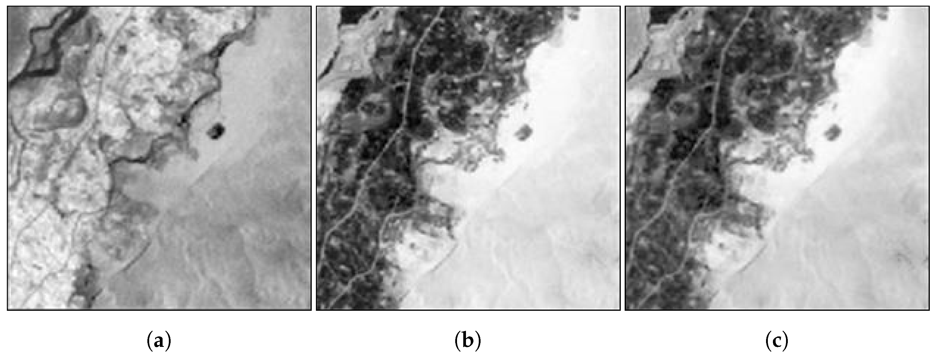
2.4. Image Features for Agricultural Land Classification and Input Standardisation

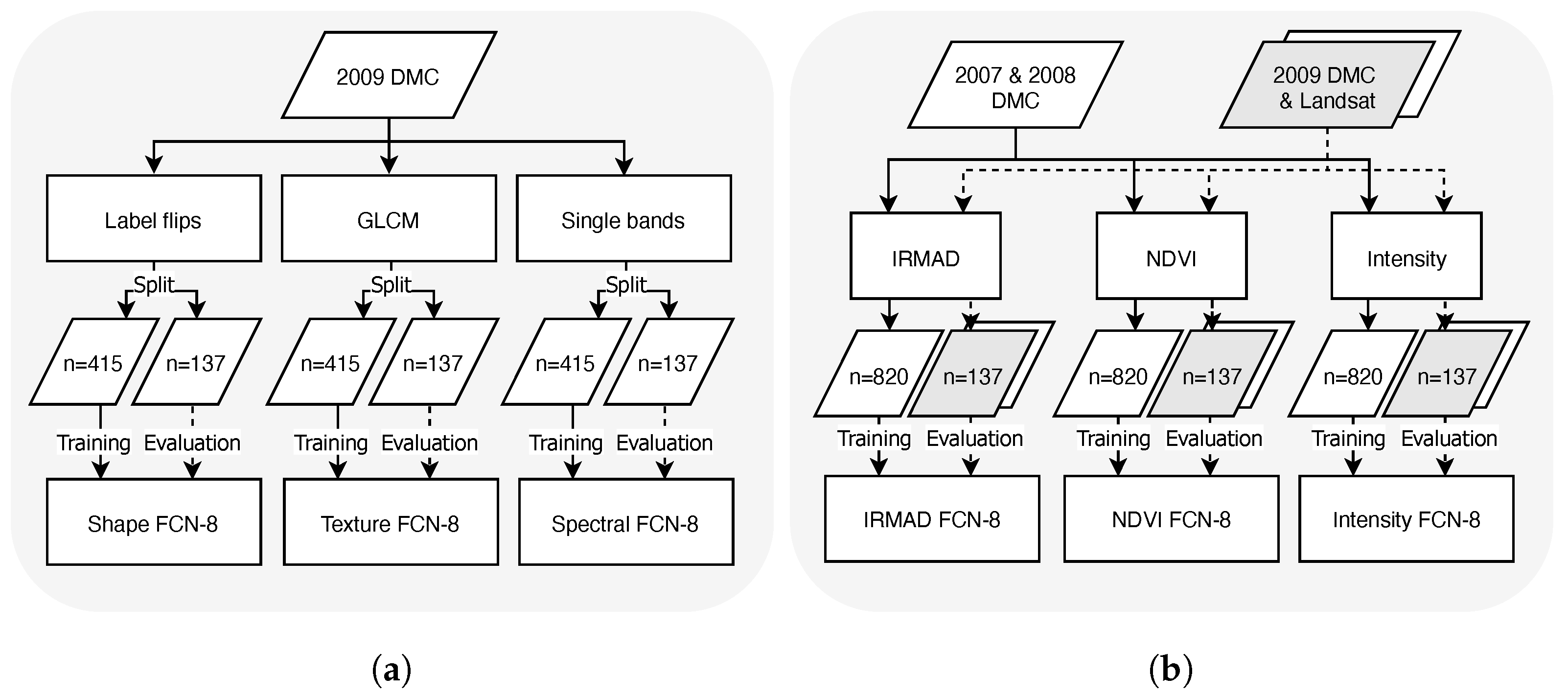
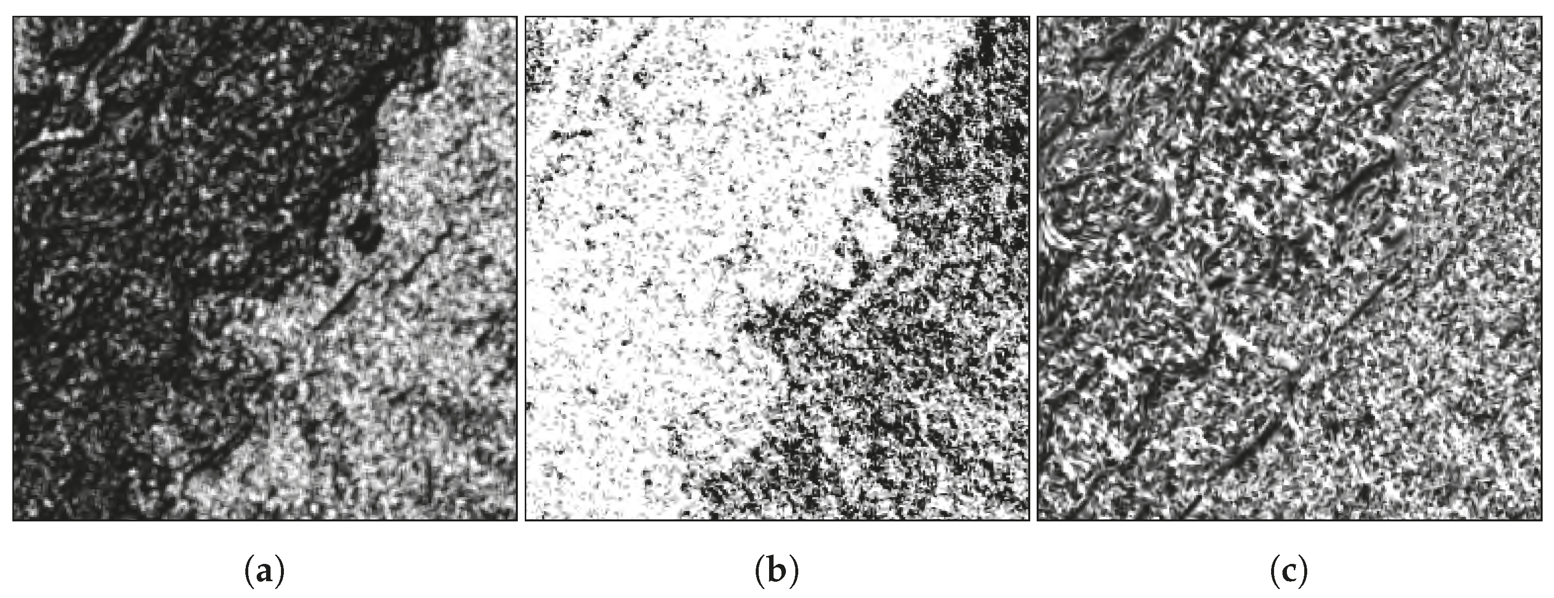
Image features and image standardisation were investigated in order to optimise transfer learning of the generalised model from the variable sources of input data (Figure 3). Isolating the individual effect of spectral reflectance, textural or spatial patterns, and shape on model accuracy is complex as these features are combined by the convolutional layers of the FCN-8. The approach taken was to create sets of the 2009 training data (number of samples, n = 415), using DMC Level 1A image chips, with the feature of interest extracted to train separate models (steps shown in Figure 3a). The individual models were evaluated on the 2009 validation samples (n = 137) from the targeted sample strategy.

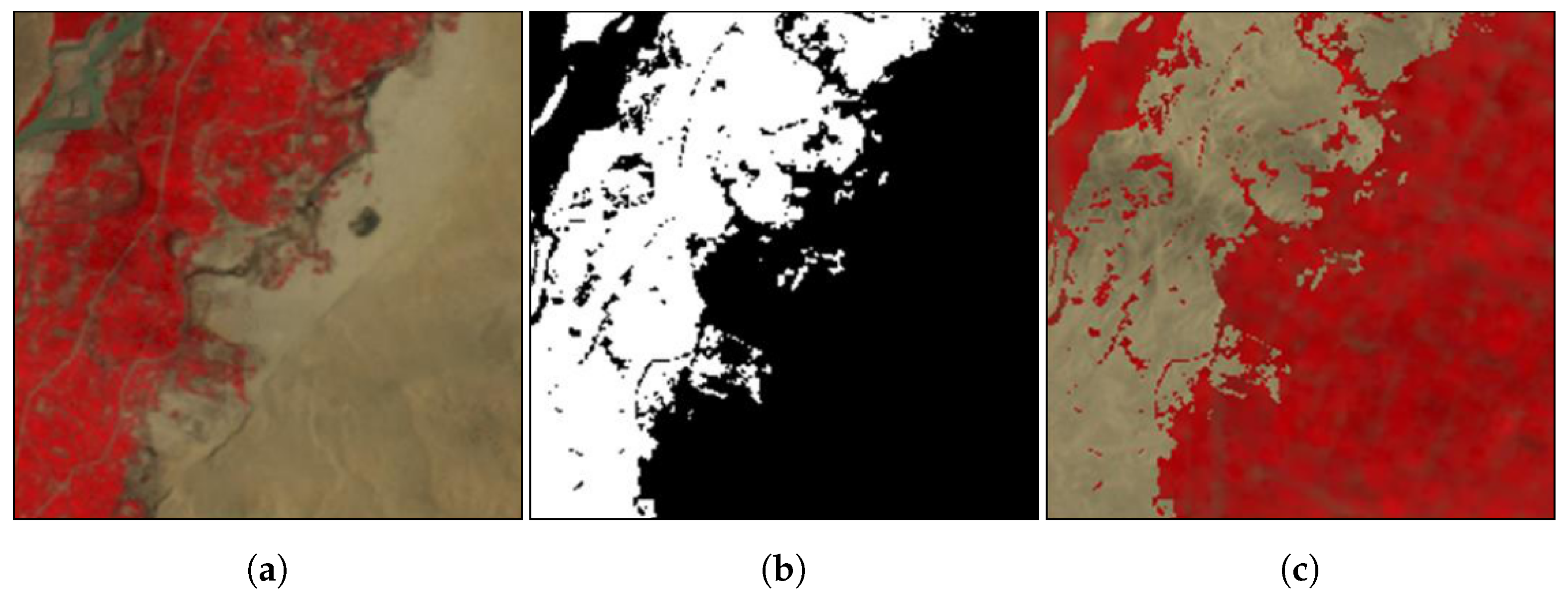
The model for the shape was trained on a synthetic dataset created using a similar method to that in [23], where input images were modified by randomly switching the pixel values to those of the another class. The reasoning behind the approach is that if pixel values within an object are no longer related to the class label, the CNN can only learn to separate classes based on the shape of objects. The 2009 training samples were ordered based on the proportion of agriculture, and in every other sample the pixels were swapped to those from the other class (Figure 4). Replacement pixels were taken from samples with 100% background and 100% agriculture, selected randomly. The combined synthetic and Level-1A samples were used to train an FCN-8 model over 50 epochs.

Textural components were extracted by applying a grey-level co-occurrence matrix (GLCM) to the sample images [24]. The textural metrics with the greatest variance, homogeneity, entropy and correlation, were used as a three band input (Figure 5), in place of the FCC, for each sample to train an FCN-8 model over 50 epochs, with:

$$\mathrm{Homogeneity}=\sum _{i,j=0}^{N-1}\left(\frac{P_{i,j}}{1+{(i-j)}^2}\right),$$

(2)

$$\mathrm{Entropy}=\sum _{i,j=0}^{N-1}{P}_{i,j}(-ln{P}_{i,j}),$$

(3)

$$\mathrm{Correlation}=\sum _{i,j=0}^{N-1}{P}_{i,j}\left[\frac{(i-{\mu }_i)(j-{\mu }_j)}{\sqrt{\left({\sigma }_i^2\right)\left({\sigma }_j^2\right)}}\right],$$

(4)

where $P_{i,j}$ is the probability of column i and row j values occurring in adjacent pixels using the fixed kernel window of the GLCM, $\mu$ is the mean, and $\sigma$ is the standard deviation [25].

Separating spectral features from their texture was not possible while maintaining the size of the input sample images. Instead, FCN-8 models were trained on sample sets of single band inputs (Figure 6) from the FCC over 50 epochs and compared to the models trained on isolated features of texture. The difference in accuracy between the individual band models and the previous texture models was attributed to the effect of spectral information.

Standardisation of input data was investigated for minimising the variation in measured surface reflectance caused by atmospheric, topographic and illumination differences between images. This is an important, and often overlooked, source of spatial and temporal variation in image pixels used for deep learning. Four approaches were selected: (1) Top of Atmosphere (TOA) reflectance calibration (Level-1A), (2) Iteratively Reweighted Multivariate Alteration Detection (IR-MAD), (3) pixel intensity, and (4) NDVI. Image data for Landsat and Sentinel were downloaded as pre-processed Level-1A and DMC images were pre-calibrated to TOA using:

$${\rho }_{\lambda }=\frac{L_{\lambda }{d}_{ES}^2\pi }{E_{\lambda }cos\left({\theta }_s\right)},$$

(5)

where ${\rho }_{\lambda }$ is the spectral reflectance, $L_{\lambda }$ is the spectral radiance, $d_{ES}$ is the Earth–Sun distance, $E_{\lambda }$ is the mean solar exo-atmospheric spectral irradiance and ${\theta }_s$ is the solar zenith.

IR-MAD is a radiometric transform for extracting invariant pixels from two images to determine normalization coefficients (slope, intercept) from orthogonal regression, described fully in [26]. The approach uses Canonical Correlation Analysis (CCA) to find the vector coefficients (a and b) that maximise the variance of the difference between two N-dimension images (F and G). The MAD variates (M) are constructed from the paired differences of the transformed images $U=a^{T}F$ and $V=b^{T}G$:

$$M_i=U_{N-i+1}-V_{N-i+1},i=1,\dots ,N.$$

(6)

The probability of change (Z) can be estimated from the sum of the squares of the standardised MAD variates:

$$Z=\sum _{i-1}^N{\left(\frac{M_i}{{\sigma }_{M_i}}\right)}^2,$$

(7)

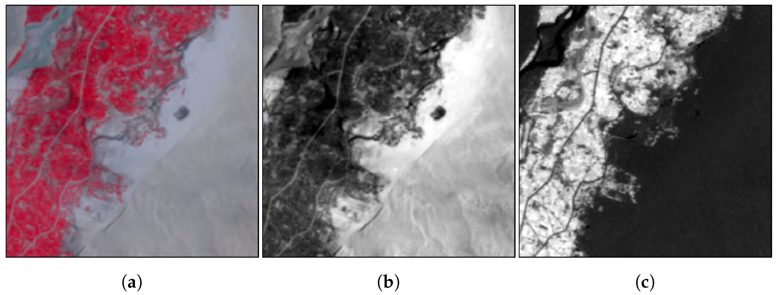
where $\sigma$ is the standard deviation. Invariant pixels between both images can then be extracted using a 95% threshold of no-change.

Sets of standardised image samples were created from the 2007 and 2008 DMC images for training individual FCN-8 models for each approach (Figure 7) and validated on DMC and Landsat-5 images from 2009 (steps shown in Figure 3b). For the IR-MAD normalised set, images were resampled to the same 32 m pixel grid and normalised to a target DMC image from 27 April 2007 using code from [27] (available at https://github.com/mortcanty/CRCPython (accessed on 2 August 2023)). Image chips were then extracted at the sample locations for model training (n = 820). Validation samples (n = 137) were extracted from 2009 DMC and Landsat-5 images, and were normalised using the same target DMC image. No Landsat-5 data were used in training this model.

NDVI and intensity sets were created from the Level-1A samples, with pixel intensity calculated as the weighted sum of the spectral image bands. Individual models were trained using the same 2007 and 2008 sample locations and validated on 2009 DMC and Landsat-5 images, again with no Landsat-5 data used during training.

2.5. Building a Generalised Model with Dense and Sparse Labels

A generalised model was developed by transfer learning across multiple yearly datasets from DMC and Landsat-8 using a combination of dense and sparsely labelled samples. All images were first pre-processed to standardise inputs using IR-MAD normalisation, detailed in Section 2.4. The first step in model development was training a base model using the densely labelled DMC data from 2008 to 2009 and the targeted sample strategy. The model was then fine tuned on Landsat-8 OLI imagery used by the UNODC from 2015 to 2019 in the creation of their potential agmask. This cumulative training strategy was designed to replicate a process of year-on-year fine tuning of the model.

Labelling the Landsat-8 image data was problematic as the UNODC agmasks contain land not in production within the current year that would be labelled as agriculture in the images. Manual editing of the samples from the 2015 UNODC potential mask was carried out to remove areas not in production and check consistency with the DMC agmasks. A random subset of 25% of the 273 training samples were used to fine tune the base model, as suggested by Hamer et al. [6], and were validated using a hold out set of 91 samples.

A sparse labelling procedure was trialed for fine tuning the model on the 2016 and 2017 UNODC data to investigate if non-contiguous blocks of pixels within the samples could be used for training. New areas of agriculture for each year were isolated from the agmasks by intersection to ensure only active agriculture was included in the agricultural class. The data was labelled as new agriculture, background or unknown using the agmask from the year of training and the previous year. A new layer was then added to the sample to weight the cost function, setting new agriculture and the background class to 1 and all other pixels to 0, in a similar approach used to balance samples in Long et al. [17]. Samples containing no new agriculture (>1%) were removed from the training sets. The same validation sample locations (n = 91) were used for evaluating the generalised model for 2015 to 2017, with fallow areas edited out manually. Model accuracy was evaluated before and after fine tuning over 50 epochs and on Sentinel-2 images from 2017 with no further training.

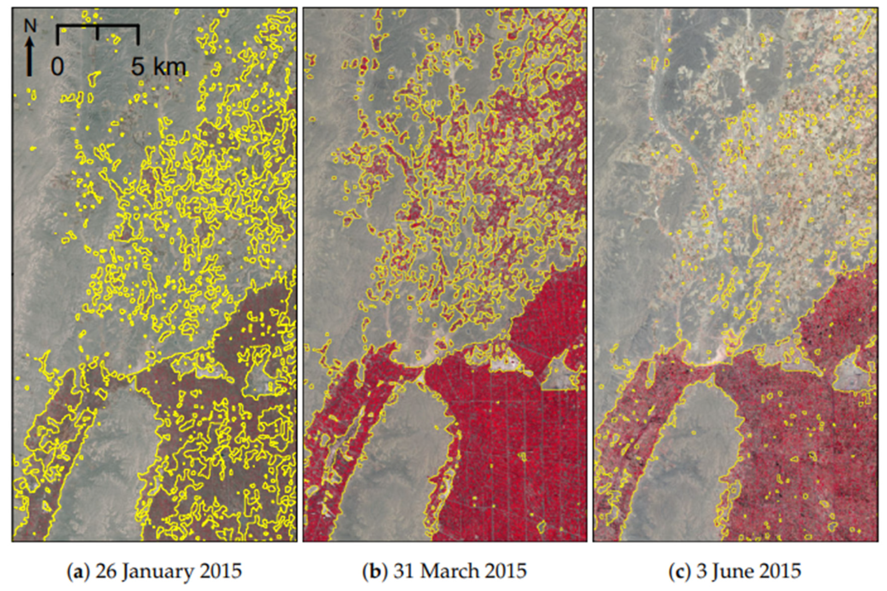
2.6. Image Timing

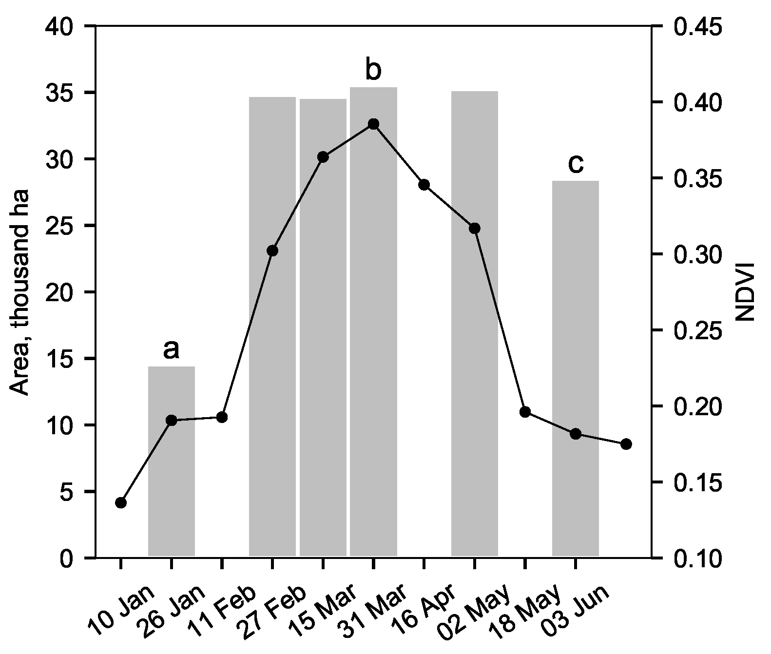
The effect of image timing on classification was investigated to determine the operational time-window for image collection, which is an important operational parameter for the generalised model as it defines the earliest point in the growth cycle that accurate information on agricultural land can be collected for the current year. A time series of largely cloud-free Landsat-8 images from 2015 were selected that covered the first crop growth cycle in Helmand, from January to June (Table 1). Each input image was normalised to the target DMC image from 2009 using invariant pixels identified automatically using IR-MAD and was then classified using the FCN-8 model, fine tuned up to 2015 (see Section 2.5). The area of agriculture within the same set of cloud-free 2015 validation samples (n = 91) was calculated for each classified image.

Crop phenology for the same period was estimated from a time series of NDVI Landsat-8 OLI images from Google Earth Engine. The mean NDVI was calculated for each time point within the agricultural area of the samples at the maximum extent for 2015 (31 March image).

2.7. Land Use Change in Helmand Province

The generalised FCN-8 model developed in Section 2.5 was used to classify agricultural land in Helmand Province to map the spatial and temporal variation in land under cultivation (active agriculture) each year between 2010 and 2019. Medium resolution cloud-free images from Landsat or Sentinel-2a for each year were selected at dates close to the peak in vegetation activity (

Table 2. Images used for production of yearly agricultural masks using the generalised FCN-8 model for Helmand Province from 2010 to 2019. Images timed to peak vegetation response.

Year	Image Sensor	Image Dates
2010	Landsat-5	8 March & 2 April
2011	Landsat-5	20 March & 12 April
2013	Landsat-8	10 April & 26 April
2014	Landsat-8	3 March & 28 Mar
2015	Landsat-8	7 April & 16 April
2016	Landsat-8	24 March & 18 April
2017	Sentinel-2	8 April & 15 April
2018	Sentinel-2	31 March & 3 April
2019	Sentinel-2	29 March & 5 April

) and processed to standardised reflectance using IR-MAD (see Section 2.4). No suitable images were available for 2012 because of the limited acquisitions during the decommission period of Landsat-5. Sentinel-2 imagery was resampled to the same resolution as Landsat imagery (30 m) for consistency in reporting total agricultural area and comparison over the time-series.

2.8. Hindcasting and Application in Other Areas

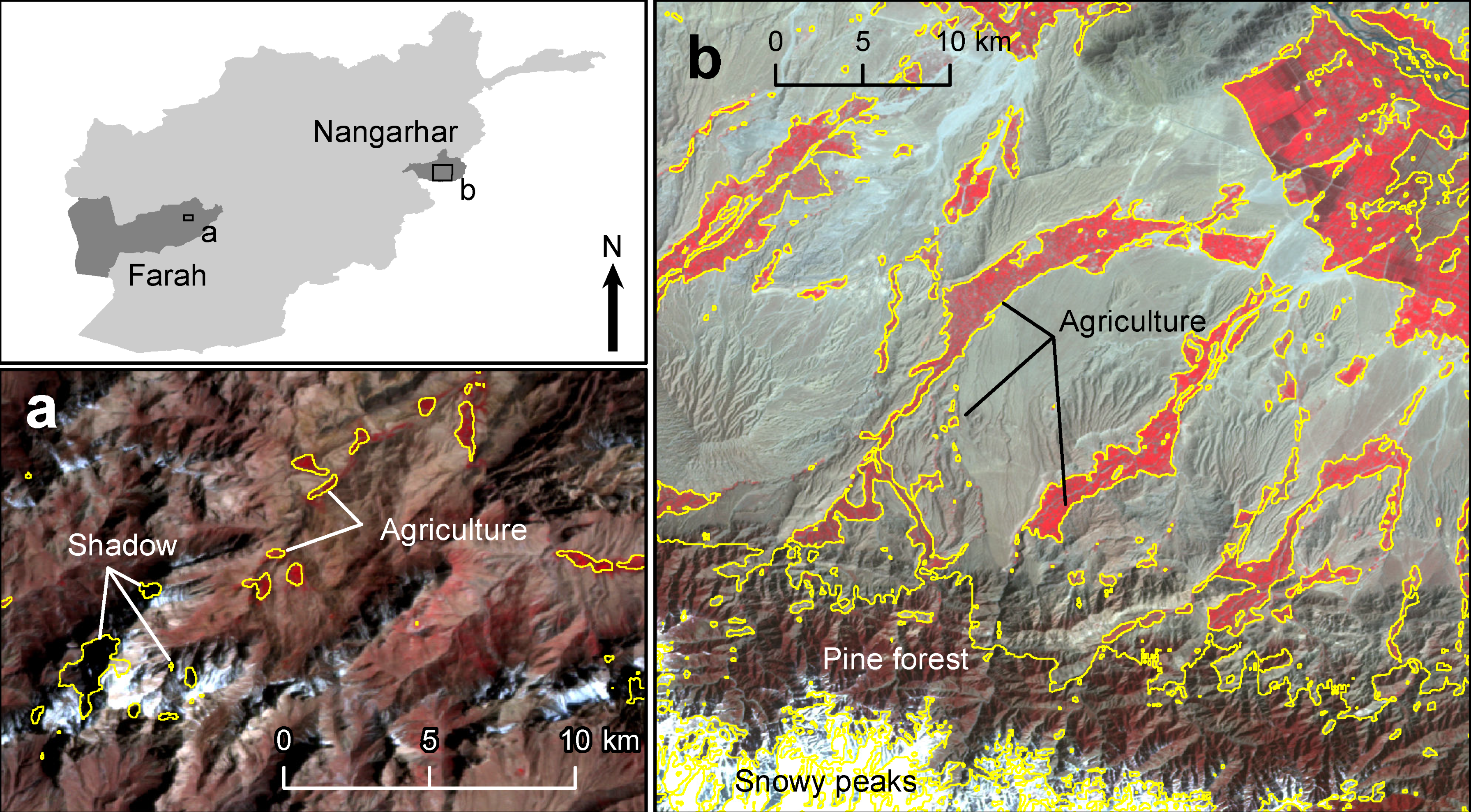
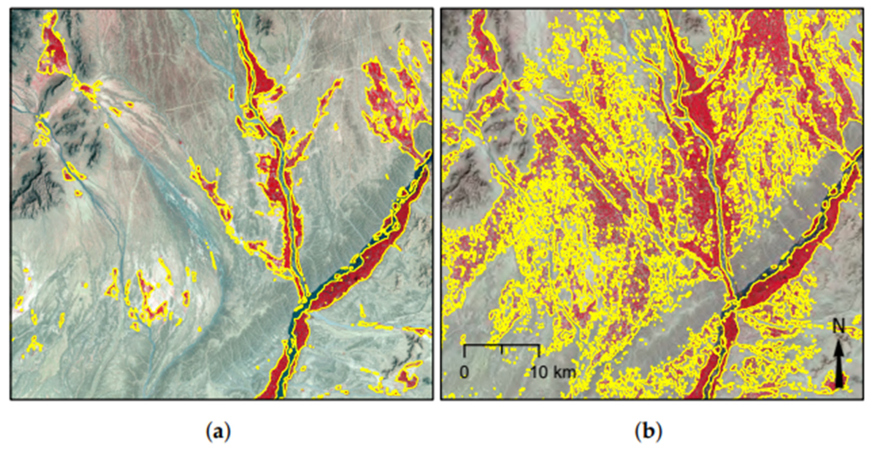
The generalised FCN-8 model was tested on imagery well outside the temporal range of the training data in Helmand Province, and outside the geographical range of the training data in Farah and Nangarhar Provinces. The model was hindcast, defined as the use of a model to re-create past conditions, on a Landsat-5 image collected on 18 April 1990, calibrated to reflectance using IR-MAD (Section 2.4) with no further training. The Farah and Nangarhar images were the same DMC scenes used to create the original 2008 agmasks collected on 5 April 2008 and 22 March 2008, respectively. The images were calibrated to TOA reflectance and classified using the generalised model. The classification accuracy was evaluated against a random 10% sample of pixels from the existing agricultural masks for 2008, which were created using the same manual process as the historical Helmand agmasks. Again no further training took place.

2.9. Model Validation

Land cover classification accuracy was assessed using the hold-out validation samples as reference data to calculate standard accuracy metrics at the pixel level. Overall accuracy (OA) is the number of correctly classified pixels in comparison to the reference data and widely adopted within remote sensing [28]:

$$\mathrm{OA}=\frac{{\sum }_i{n}_{i,i}}{{\sum }_i{t}_i},$$

(8)

where $n_{i,i}$ is number of pixels predicted as class i belonging to class i and $t_i$ is the total number of pixels belonging to class i in the reference data.

Producer accuracy (PA) is the percentage of correctly classified pixels within each class in the evaluation data (omission errors in the classification), also known as recall for positive cases [29],

$${\mathrm{PA}}_i=\frac{n_{i,i}}{{\sum }_i{n}_{j,i}},$$

(9)

where $n_{j,i}$ is the number of pixels predicted as class j belonging to class i.

User accuracy (UA) is the mapping accuracy for each class (commission errors in the classification), also known as precision for positive cases [29],

$${\mathrm{UA}}_i=\frac{n_{i,i}}{t_i}.$$

(10)

The agreement between predicted and reference pixels in overlapping regions was assessed using the frequency-weighted Intersection over Union (fwIoU) [30]:

$$\mathrm{fwIoU}=\frac{1}{{\sum }_i{t}_i}\sum _i\frac{t_i{n}_{i,i}}{t_i+{\sum }_j{n}_{j,i}-n_{i,i}}.$$

(11)

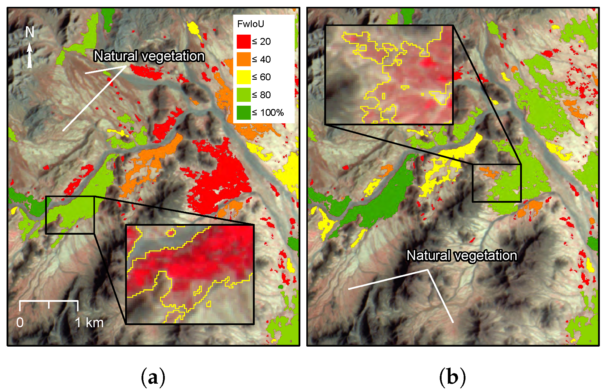
A new method for mapping fwIoU at the level of individual objects was developed to assess how agreement varied spatially and with object size. Individual objects, defined as any region with more than one connected pixel, were first subset from the reference agricultural masks. Each object was matched to zero or more objects in the classified output by intersection. FwIoU was then calculated and for each set of matching objects within the bounding box of the reference object in order to map agreement in overlap of agriculture between the classified and reference data.

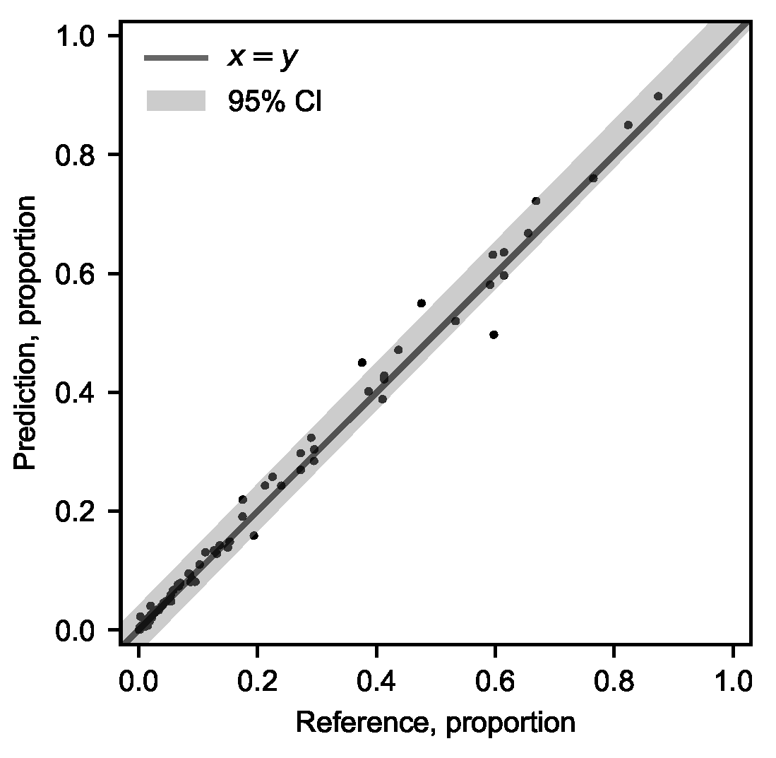
The confidence of agricultural land prediction from the generalised FCN-8 model was calculated as

$$\widehat{y}\pm t_{1-\alpha /2,n-2}\sqrt{\mathrm{MSE}\left(1+\frac{1}{n}+\frac{{(x_h-\overline{x})}^2}{{\sum }_i{(x_i-\overline{x})}^2}\right)},$$

(12)

where $x_i$ is the proportion of agriculture in the validation sample i with mean $\overline{x}$, $y_i$ is the model prediction for the validation sample i, $t_{1-\alpha /2,n-2}$ is the critical value from a t-distribution, $\widehat{y}$ is the fitted value at $x_h$ from orthogonal least squares regression, and n is the number of samples. $\mathrm{MSE}$ is mean square error of the prediction,

$$\mathrm{MSE}=\frac{{\sum }_i{(y_i-\widehat{y})}^2}{n-2}.$$

(13)

The kappa coefficient [31], used to assess aclassifier performance devoid of chance agreement, was not calculated in this study as there is disagreement on its use relating to assumptions of randomness in validation data [29,32,33].

3. Results

3.1. Image Features for Agricultural Land Classification

Models trained using isolated image features (shape, texture and spectra) were investigated in order to identify diagnostic features of agricultural land in input images (

Table 3. Effect of isolated image features on overall classification accuracy (OA) and frequency weighted intersection over union (fwIoU). Synthetic shape dataset, three-band texture dataset (homogeneity, entropy, correlation), and individual near-infrared (NIR), red, and green bands, benchmarked against the three-band level-1A DMC dataset using the 2009 FCN-8 model. Training sample n = 415, validation sample n = 137.

Feature Dataset	OA (%)	FwIoU (%)
Level-1A (benchmark)	93.74	65.51
Shape	53.20	12.84
Texture	72.87	55.27
NIR band	73.65	56.25
Red band	87.77	62.78
Green band	86.77	61.84

). The three-band texture model had similar OA and fwIoU to the single band NIR model, showing that the FCN-8 model is able to separate agriculture from the background class based largely on their textural differences (OA of ∼73%). The combined spectral and textural information in the level-1A data increased the OA by 20% and fwIoU by 10%. The effect of shape on model performance was minimal, with poor classification accuracy (53%) and very low fwIoU (13%).

3.2. Transfer Learning between Sensors

The validation accuracy of input standardisation methods for transfer learning between DMC and Landat-5 imagery are shown in

Table 4. Effect of image standardisation method on overall accuracy (OA) and frequency-weighted intersection over union (fwIoU) for FCN-8 models trained using calibrated reflectance (IR-MAD), top of atmosphere reflectance (Level-1A), NDVI and single band intensity images from 2007 and 2008 DMC images and evaluated on DMC and Landsat-5 images from 2009.

Standardised Input	Image Type	OA (%)	FwIoU (%)
IR-MAD	DMC	94.49	67.96
	Landsat-5	93.98	62.84
Level-1A	DMC	94.39	67.21
	Landsat-5	92.01	57.64
NDVI	DMC	93.44	65.89
	Landsat-5	91.67	55.12
Intensity	DMC	91.87	57.81
	Landsat-5	89.96	53.15

. Reflectance data from the three band images (level-1A and IR-MAD) from DMC and Landsat-5 had higher OA and fwIoU compared to the single band normalising using NDVI or intensity. Reflectance matching between images using invariant pixels (IR-MAD) resulted in a small increase of OA and fwIoU compared with the top of atmosphere reflectance data (level-1A). Further visual comparison of agmasks identified improved classification at boundaries and areas with gradual changes from agriculture to desert for reflectance-matched images (IR-MAD) compared to level-1A reflectance. This boundary effect is shown in the results for localised fwIoU calculated for each group of contiguous pixels, where the improvement in output from the matched images is related to the complexity of the boundary of the block (Figure 8). The best result, found using three band reflectance images normalised to a target scene using IR-MAD, was applied to standardise the input images for training the generalised model.

3.3. Generalised Model

The generalised model had high accuracy and reached a relatively stable OA, UA and PA (>95%, >91%, and >85%, respectively) after fine tuning on 2007 to 2009 DMC and 2015 Landsat-8 (

Table 5. FCN-8 model overall accuracy (OA) and agricultural class user accuracy (UA) and producer accuracy (PA) between 2015 and 2017 before and after fine tuning with sparse Landsat-8 and Sentinel-2 datasets. Crosses (×) indicate cumulative transfer learning, for example: in the first row the model was trained on DMC data (2007 to 2009) and evaluated using 2015 Landsat-8, in the second row the DMC trained model was updated and evaluated using 2015 Landsat-8.

Sensor	Year	Training Dataset				OA	UA	PA
		DMC	2015	2016	2017	(%)	(%)	(%)
Landsat-8	2015	×				90.99	89.32	83.81
Landsat-8	2015	×	×			93.01	91.76	87.54
Landsat-8	2016	×	×			95.12	91.34	89.11
Landsat-8	2016	×	×	×		96.11	92.01	89.55
Landsat-8	2017	×	×	×		95.01	91.26	85.71
Landsat-8	2017	×	×	×	×	95.98	91.91	89.03
Sentinel-2	2017	×	×	×	×	95.58	91.23	88.81

). From 2016 onwards, the OA, UA and PA were consistent before and after fine tuning, except for the PA in 2017, which dropped by 5% before increasing after fine tuning on sparse data from the same year. The generalised model, trained up to 2017, had similar OA, UA, and PA on Landsat-8 and Sentinel-2 (resampled to 30 m) without any fine tuning using Sentinel-2 data.

A comparison of the results of the generalised FCN-8 model with the reference data from 2009, 2015, 2016, and 2017 validation samples shows close agreement in agricultural land classification with a small but increasing positive bias (up to 3%) for samples containing a high proportion of agriculture (Figure 9). The 95% confidence interval for classification using the general model was ±4%, calculated based on a proportion of 0.06 of agriculture, which is representative of Helmand Province.

3.4. Image Timing

Classification of standardised Landsat-8 images from 2015 using the generalised model show variation in the agricultural area according to crop development measured using NDVI (Figure 10). Early in the season, before green-up of the annual crops, the model underestimates the agricultural area as the vegetation response is weak because individual plants are small (Figure 11a). The classified area increases rapidly once plant canopies begin to develop and is close to the maximum (Figure 11b) at 50% of the peak NDVI at 27 February (Figure 10). The classified area reduces after first cycle crops have senesced (Figure 11c), indicated by a sharp fall in NDVI (Figure 10). These results show a timing window for image collection of three weeks either side of the peak in vegetation activity, with images close to the peak giving the largest overall agricultural extent.

3.5. Mapping Agricultural Expansion

Classification of images between 2010 and 2019, using the generalised model, showed an increasing trend in the area of land under active agricultural use since 2010 (Figure 12). The majority of this expansion can be seen in the area north of the canal, which was desert in 1990 (inset box in Figure 13).

3.6. Use Outside Helmand

The generalised model was able to accurately classify agricultural land in Farah and the main river valley in Nargarhar in similar landscapes to Helmand (

Table 6. FCN-8 generalised-model overall accuracy (OA), agricultural class user accuracy (UA), and producer accuracy (PA) using DMC imagery in Farah and Nangarhar Provinces outside of the area used for model development. Calculated from a 10% random sample of pixels from the original 2008 manually edited agmasks in both provinces. The low UA for Nangarhar was caused by commission of pine needle forests (shown in Figure 14), a landcover not present in the data used for model training.

Province	DMC Image Date	OA (%)	UA (%)	PA (%)
Farah	5 April 2008	99.55	80.49	78.02
Nangarhar	22 March 2008	88.44	38.20	69.02

). The UA and PA for Farah was lower than for the Helmand data because of classification errors in the mountainous northern part of the Province. Results were similar in Nangarhar in the main valley and ribbon valleys extending south towards the mountains. There was confusion on the slopes of upland areas, with the generalised model classifying significant areas of sparse natural vegetation as agriculture (Figure 14). On closer inspection, these areas were found to be a class of pine-needle forest that is not found in Helmand Province, where the model was trained.

4. Discussion

There are major limitations to overcome in order to create a robust model that is capable of classifying the latest satellite image into an accurate map of land-cover. These are caused by the radiometric and atmospheric differences between images, alongside the natural variation in environmental conditions that affect growth and phenology [34,35]. The improved performance of CNNs and deep learning over other machine learning approaches, such as Random Forest, is attributed to their ability to efficiently encode the contextual information that is less affected by changes in absolute pixel values [6,36]. Our results show that the textural features related to agricultural land use are consistent between images at medium resolution and alone can reach an overall classification accuracy of 73% for images collected in different years (see Table 3). This explains why the FCN-8 model is able to separate natural vegetation from agricultural land even though the spectral response of the land-cover at the pixel level is similar at medium resolution. However, the highest classification accuracy (>95%) was achieved using the full three-band image (NIR, R, G), which combines spatial and spectral image features.

It is interesting to note that shape plays no role in the classification (OA of 53%). This is perhaps not surprising, as the appearance of agricultural areas in medium resolution imagery is not distinct. At higher resolutions, features such as the shape of field parcels would be visible to the model and expected to play a greater role in discrimination of agricultural land, as can be demonstrated in segmentation of objects in natural photography [17].

Transforming images into a lower number of input features was investigated as a way to standardise the input to the FCN and to reduce the complexity. Models using NDVI or single-band intensity resulted in lower classification accuracy (1–2%) compared to using the three band image, suggesting that there is data loss when reducing the number of bands. Conversely, expanding the number of input dimensions into the short-wave infrared could improve the classification but was not investigated in this study as there were only three bands in the DMC imagery used to train the model between 2007 and 2009. One approach for adding spectral information to the model would be to initialise extra input dimensions for the short-wave bands from Landsat-8 and Sentinel-2 using weights cloned from other input layers during transfer learning. Further work is needed to understand the input features that are diagnostics of land-cover and land use classes and to take advantage of the full range of spectral data to build more efficient models.

The input data for FCNs are normalised to maintain consistency in colour values and reduce variability. Normalisation will also stabilise and speed up model convergence during training [37]. For 8-bit natural photography, which FCN models were originally developed for, this is normally done by scaling and centring the values using the mean and variance of the whole dataset. This approach is not ideal for EO data as images will typically have different dynamic range and the distribution of spectral response will vary with landscape. In this study we used reflectance, which reduces the sensor and illumination effects and scales the input appropriately for use in the FCN while preserving the spectral properties of the image.

The effect of further normalisation of the TOA, using IR-MAD to match radiometry based on invariant pixels, can be seen as an improvement in classification at the edges of marginal agriculture, where a small change in value can switch a pixel between the agricultural or non-agricultural class. These differences have a small effect on the overall accuracy in Helmand Province, as the majority of the land used for agriculture has a distinct boundary because of irrigation features. However, in other areas or for wider applications without such clear delineations, like mosaic classes or transitions between complex classes, standardising image radiometry will have a significant effect on the ability of FCN models to generalise.

Relative normalisation was used instead of an absolute radiometric calibration with an atmospheric model as no in-situ measurements, or approximations for historical images, are required and potential differences in sensor-calibration can be avoided [38]. IR-MAD has also been shown to reduce variability in retrieval of surface parameters compared to absolute correction [39]. Absolute atmospheric correction is worth investigation going forward as it will remove the need for reference images and any potential distortions in temporal patterns [40].

The FCN’s ability to be trained through transfer learning makes it well suited to developing a generalised model across image sensors from existing datasets. Firstly, the model can be trained from a much broader range of examples as training takes place incrementally, while the model from the previous step is maintained. Secondly, the ability to fine tune using a much smaller dataset means that any manual labelling effort is reduced once a base model has been trained. The use of sparse data, where training samples contain unlabelled (unknown) areas instead of spatially dense labels, means data from a wider range of sources can be used for training and fine tuning.

Single-date images were used instead of multi-temporal data as classification has to work in near real-time throughout the season. The model was found to be robust to changes in image acquisition date up to 2 months either side of the peak in vegetation activity, measured using NDVI. This is an important consideration for operational use as obtaining information on land use early in the season can improve the efficiency of the UNODC’s opium survey, either by reducing the size of the sample frame in areas that are not active, or extending sampling into new areas. Early warnings of changes are also invaluable for directing resources to investigate new trends in opium production within the same season. Tracking the development of agriculture in near real-time using the generalised model is timely and efficient as all steps in the classification pipeline can be automated and inference is fast.

A small bias in classification is visible in larger blocks of agriculture that contain many gaps between fields parcels. This is caused by the loss of resolution that at takes place during the resampling and de-convolution steps in the FCN-8 model. This is a limitation of the model and leads to generalisation in areas of high complexity at the boundary between agriculture and the background land-cover. Further research into model refinement using the full spatial resolution of Sentinel-2 (10 m) is recommended to reduce this effect and improve the resolution of the mapping.

Boundary generalisation may also be caused by differences in the original image interpretations used for labelling. While quality control using cross-checking was undertaken in the production of these historical data, there are differing levels of uncertainty, especially in more complex areas where considerably more effort is required to fully digitise boundaries.

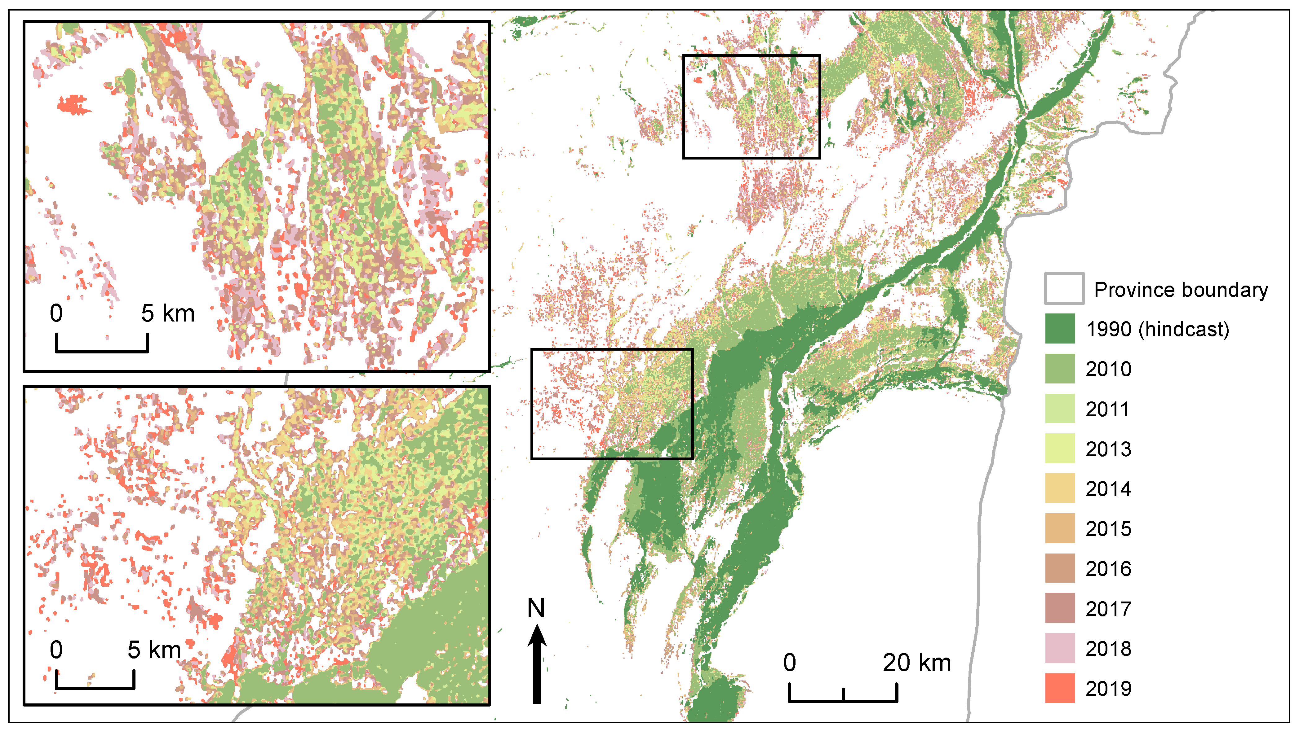
Mapping using the generalised model provides much greater insight into the annual variation in land use compared to the potential agmask, which is the result of adding new areas to an existing map. Important changes related to water availability, salinity and the consistency of irrigated areas reveal information that can be used to investigate the links between opium production, water use, and food security. Mapping the active area can also be used to validate that well-driven expansion into the desert is increasing the overall area of land, and the overall demand for irrigation water, and is not a shift in the location of production. Going further back in time by hindcasting the model also reveals how areas have seen significant growth in agricultural production since the 1990s (Figure 15).

Our results show that the ability of the model to generalise is directly linked to the landscapes encountered during training. In Farah and Nangarhar the classified agricultural area was consistent with manual interpretation in the main growing areas and narrow ribbon valleys that follow rivers into more mountainous areas. The classified area contained a number of false positives as the terrain within the images varied in appearance from the original Helmand training data. In Nangarhar there were larger areas of confusion linked to distinct tree-covered uplands. Use of the generalised model in new areas is an improvement over manual methods and supervised classification approaches based on the analysis of single images, because of the much reduced effort of collecting additional training data for fine tuning. For example, digitising additional samples in problem areas would require minimal manual work to produce an accurate map compared to producing a province-level agmask from scratch. One suggested improvement is to identify those areas in the output with lower classification confidence for further fine tuning, taking the approach closer to a self-learning system.

5. Conclusions

A generalised deep learning model was developed for classification of agricultural land in Afghanistan from medium resolution satellite imagery. The accuracy was comparable to that of manual image interpretation (>95%) but without further training, so the approach can provide rapid information on land use and land use change much earlier in the season with minimal manual input from analysts. High classification accuracy across years and between sensors was related to textural image features (∼73% of overall accuracy) and normalising images to reflectance. The model can be adapted for new landscapes by fine tuning with smaller datasets using sparse observations. The model is sensor-agnostic and can be used on new and archive images from different sensors (tested on DMC, Landsat 5 and 8, and Sentinel-2) to reveal long term trends ($\pm 4\%$ confidence intervals) in land use.

Image pre-processing and classification can be fully automated for use as operational tools for improving the sampling efficiency of the UNODC’s annual opium survey and can provide timely maps of changes in the total area of production, which present key information for assessing the impact of opium cultivation on Afghanistan’s agricultural system. The findings of this study demonstrate how transferring information between sensors and across years makes significantly more training data available for deep learning and opens up exciting new opportunities for monitoring agricultural change more accurately, for the automation of image classification tasks more generally for both new and long-term EO programmes, to improve our understanding of the environment.