Abstract
Agricultural cropping intensity plays an important role in evaluating the food security and the sustainable development of agriculture. The existing indicators measuring cropping intensity include cropping frequency and multiple cropping index. As a nominal measurement, cropping frequency classifies crop patterns into single-cropping and/or double-cropping and leads to information loss. Multiple cropping index is calculated on the basis of statistical data, ignoring the spatial heterogeneity within the administrative region. Neither of these indicators can meet the requirements of precision agriculture, and new methods for fine cropping intensity mapping are still lacking. Time series remote sensing data provide vegetation phenology information and reveal temporal development of vegetation, which can be used to facilitate the fine cropping intensity mapping. In this study, a new temporal mixture analysis method is introduced to estimate the abundance level cropping intensity from time series remote sensing data. By analyzing phenological characteristics of major land-cover types in time series vegetatiosacan indices, a novel feature space was constructed by using the selected PCA components, and three unique endmembers (double-cropping, natural vegetations and water bodies) were found. Then, a linear spectral mixture analysis model was applied to decompose mixed pixels by replacing spectral data with multi-temporal data. The spatio-temporal continuous, fine resolution, abundance level cropping intensity maps were produced for the North China Plain and the middle and lower reaches of the Yangtze River Valley. The experiments indicate a good result at both county and pixel level validation. The method of manually delineating endmembers can well balance the accuracy and efficiency. We also found the size of the study area has little effect on the unmixing accuracy. The results demonstrated that the proposed method can model cropping intensity finely at large scale and long temporal span, at the same time with high efficiency and ease of implementation.
1. Introduction
Agricultural production is the cornerstone for the survival and development of human beings [1]. Due to the impact of urbanization, development of the market economy, the international food trade and climate change, dramatic changes have taken place in agricultural land systems. The most famous examples are the conversion of croplands into built-up areas in the Yangtze River Delta and Pearl River Delta of China [2,3], the phenomenon of double-cropping transitioning to single-cropping in the middle reaches of the Yangtze River Valley [4], the non-grain use of croplands in China [5], the collapse of soybean planting in Northeast China [6,7], and the abandoned croplands in mountainous area in South China [8]. Furthermore, locust disasters [9], armed conflict [10], COVID-19 [11,12], etc., aggravated the uncertainty of food production. The world has encountered the most serious food crisis in the past 50 years [13]. On the other hand, continuous agricultural intensification in some regions has caused serious ecological and environmental problems, such as excessive consumption of water resources [14], land degradation [15], agricultural non-point source pollution [16] and greenhouse gas emissions [17]. Therefore, agricultural cropping intensity is an important input for evaluating the sustainable development of agriculture.
The existing methods of cropping intensity mapping include cropping frequency (CF) and the multiple cropping index (MCI). The calculation of MCI is mostly based on statistical data, ignoring the spatial heterogeneity within the administrative regions [18]. CF is a nominal measurement that divides crop patterns into single-cropping and double-cropping, lacking quantitative measurement of cropping intensity. Most existing methods for mapping CF are based on counting the number of peaks in coarse resolution remote sensing images such as the Moderate Resolution Imaging Spectroradiometer (MODIS) vegetation index profiles [19,20,21,22,23]. When a coarse resolution image is used to monitor cropping frequency, the mixed pixel problem is particularly serious due to the fragmented landscapes, small patch size of croplands and complicated crop patterns in Central and South China.
There has been some progress recently on the construction of new indicators or new methods for cropping intensity mapping. Time series high-resolution images such as those from Sentinel-2 are used to monitor cropping intensity, alleviating the problem of mixed pixels to some extent [24,25,26]. However, these methods are highly dependent on data availability and constrained by complicated data pre-processing. The authors used Bayesian network to obtain cropping intensity with interval measurement using time series MODIS data [27]. This method is highly dependent on training samples, and the accuracy of the model output depends on the quality of the samples. In any case, the above existing methods of cropping intensity mapping cannot meet the requirements of precision agriculture, and new methods for fine cropping intensity mapping suitable for Central and South China are still lacking.
Although continuous accumulated high-resolution remote sensing images are helpful for precise cropping intensity mapping, this convenience has only existed since the launch of Landsat 8 in 2013 and the launch of Sentinel-2 in 2015. Medium-resolution data over long time series can bridge the gap and push back observations to the year 2000 or even earlier. Time series remote sensing data contain seasonal variation of vegetation and abundant vegetation phenology information [28]. Intra-annual dense time series images carry information on multiple cropping of crops. However, this information is usually used for crop mapping [29,30], phenology monitoring [31], etc. Vegetation phenology information contained in time series remote sensing data is not yet fully explored for cropping intensity mapping. Dense time-series remote sensing images have enough repeated observation (MODIS MOD13Q1 has 23 observations a year) and make this work possible [32].
Mixed pixels are more common in coarse resolution images and require mixture analysis technology to decompose pixels to the abundance level. There are two mixture analysis techniques: spectral mixture analysis (SMA) and temporal mixture analysis (TMA). SMA methods are generally used to decompose spectral remote sensing data, among which linear spectral mixture analysis (LSMA) is more often used. Based on the principle of SMA, TMA is a method to decompose mixed pixels by replacing spectral data with multi-temporal data.
The selection of endmembers (including their number and types) is another important issue for unmixing. The two-endmember model is suitable for the decomposition of natural land-cover types, while the three-endmember model is suitable for the decomposition of land-cover types under human disturbance [33]. For built-up areas, the most commonly used endmember selection method is the vegetation–impervious surface–soil endmember model proposed by Ridd et al. [34]. For non-built-up areas, vegetation–soil–shadow (or dry vegetation) endmember model is generally used [35]. The endmember selection is usually scene-dependent when the TMA method is used: for example, the vegetation–impervious surface–soil model [36], forests–multiple cropping–single cropping–non-vegetation model [32], and grass–corn–winter wheat–alfalfa model [37]. With proper endmember design, large scale, long temporal spans and fine cropping intensity are possible.
To aim for large-scale, long-temporal-span and fine-resolution agricultural cropping intensity estimation, this study presents a new TMA method for estimating cropping intensity from historical archived time series coarse resolution remote sensing data. The method includes: (1) constructing the feature space, finding the unique endmembers to estimate the abundance level cropping intensity; (2) exploring the feasibility of manually delineating endmembers and the effectiveness of the method on different regions with varied completeness of endmember land-cover types. This work will be of great significance for fine cropping intensity mapping at large scale and long-time series.
2. Materials and Methods
2.1. Study Area and Data
2.1.1. Study Area
The study area was the North China Plain and the middle and lower reaches of the Yangtze River Valley (Figure 1). Major land-cover types were natural vegetation, croplands, water bodies and built-up areas. Forests and scrublands were synthesized to natural vegetation since they have similar phenology. Double-cropping and single-cropping coexist in the research area. The dominant crop patterns are single-cropping paddy rice, winter wheat-soybean, winter rapeseed-paddy rice, winter wheat-maize and double-cropping paddy rice.
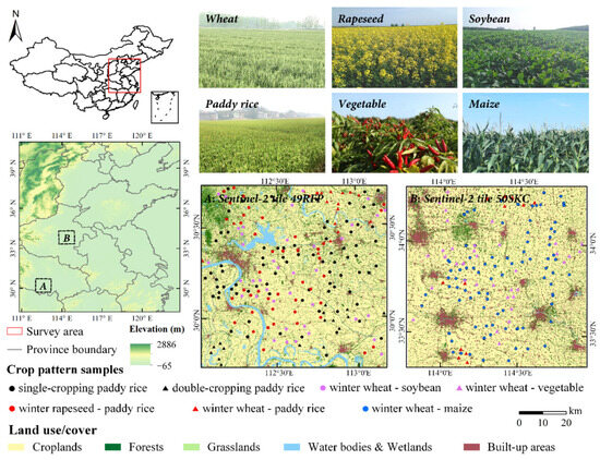
Figure 1.
The location, major land-cover types and reference samples of the study area (A and B are two test regions, corresponding to Sentinel-2 tiles 49RFP and 50SKC). The main land cover types are from the FROM-GLC10 datasets (data source: http://data.ess.tsinghua.edu.cn/, accessed on 1 March 2023) in 2017.
2.1.2. Data
MODIS MOD13Q1 Enhanced Vegetation Index (EVI) products in 2018 with 250 m resolution were used and were synthesized over 16 days based on the maximum value composite principle. The image tiles including h27v05, h27v06, h28v05, and h28v06 (h: horizontal, v: vertical) were downloaded from the National Aeronautics and Space Administration website (https://modis.gsfc.nasa.gov/, accessed on 1 March 2023). Image preprocessing, including mosaic, resampling and reprojection, was conducted using the MODIS Reprojection Tool. To eliminate the interference of clouds, snow, shadows and other factors, Savitzky–Golay filtering was adopted to reconstruct the original time series. Data quality information was extracted based on the pixel reliability layer of MOD13Q1 products.
Sentinel-2 data with a spatial resolution of 10 m were used to generate validation data. Sentinel-2A (launched 2015) and Sentinel-2B (launched 2017) sensors together offer 5-day revisit with global coverage [38]. NDVI was calculated for the Sentinel-2 data by using near infrared and red band.
Sentinel-2 NDVI composite from three key phenological phases was used to prepare the reference cropping intensity data. The first phase was in mid March, which represents the peak of the first growing season of double-cropping (termed GS1). The second phase was from late May to early June, which is the transition period between the two growing seasons (termed TGS). Both single-cropping and double-cropping had low EVI values at this stage. The third phase was in mid July, which is the peak of the second growing season of double-cropping (termed GS2). Double-cropping is shown in magenta, and single-cropping in blue in the false-color composite image (Figure 2a,b).
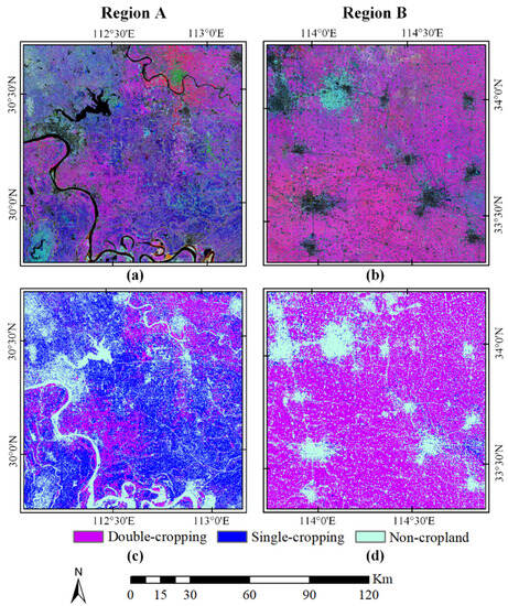
Figure 2.
Unsupervised classification of Sentinel-2 images: (a,b) are false-color composites of Sentinel-2 NDVI from three phenological phases (GS1, TGS, GS2); (c,d) are ISODATA classification results for the two regions (A) and (B).
The classification was conducted based on these NDVI composites using ISODATA, in which the classification number was between 10 and 20, and the iteration time was set to 20. The classification results were merged into three categories: double-cropping, single-cropping and non-cropland (Figure 2c,d). Finally, they were aggregated to 250 m fractional images to match the spatial resolution of MODIS data.
The crop pattern sample data were used to evaluate the accuracy of the Sentinel-2 derived cropping intensity data. The producers’ accuracies (PA) of single-cropping and double-cropping were 91.06% and 91.16%, respectively, their users’ accuracies (UA) were 92.44% and 90.58%, respectively (Table 1), and the overall accuracy (OA) and Kappa coefficient were 92.6% and 0.888, respectively, suggesting the reliability of the Sentinel-2 derived cropping intensity data.

Table 1.
Accuracies of Sentinel-2 derived cropping intensity data using crop pattern sample data.
To evaluate the accuracy of the Sentinel-2 derived cropping intensity data, we used 1779 crop samples (537 single-cropping samples, 622 double-cropping samples and 620 other samples) as reference data. These crop patterns were transferred into cropping intensity: single cropping, double cropping and other (including non-crop cultivation and non-cropland). These samples were from a filed survey in 2018 as ground truth (Figure 1), and augmented by visual interpreting high-resolution images on the Google Earth Engine platform. The ground truth data were collected using a mobile application, GPSTool 4.0. The augmentation were delineated manually by overlaying ground truth data with high-resolution images. The sample data were roughly distributed evenly throughout the validation area and were independent and identically distributed.
In addition to the Sentinel-2 derived reference data, three cropping intensity products were further used for the validation. The first was the MCD12Q2 V6 Land Cover Dynamics product, which provides global estimates of the timing of vegetation phenology at 500 m resolution [39]. The NumCycles layer in MCD12Q2 provides the total number of valid vegetation cycles in a year. The annual average of the NumCycles was calculated and then used as reference data. The second product was the Global Cropping Intensity (GCI) dataset, which is an annual global multi-cropping index distribution map covering the period from 2001 to 2019 at 250 m resolution [40]. The third was a global cropping intensity map dataset at 30 m resolution (GCI30) from 2016 to 2018 [41].
2.2. Methods
The geometric method was used to implement the TMA model. The geometric method is an important method for mixture analysis, and from a geometric perspective, the multidimensional images can be viewed as a convex simplex. The convex geometry method [42] was introduced to construct the simplex structure of time series remote sensing data in the feature space, and the endmembers were found in this feature space.
The major steps of the methodology, including feature selection, feature space construction, endmember selection, cropping intensity estimation and validation, are presented in the flowchart (Figure 3).
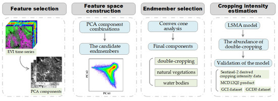
Figure 3.
Flowchart of the TMA method.
2.2.1. Feature Selection
Intra-annual time series remote sensing images provide land surface phenological information and reveal spatio-temporal development of vegetation [43]. The EVI profiles of different land-cover types demonstrated the unique phenological characteristics of double-cropping, single-cropping, evergreen forests, deciduous forests, water bodies, built-up areas, etc. (Figure 4). The temporal profiles of crops are obviously different from those of other land-cover types. Moreover, there are great differences between single-cropping and double-cropping. There are two peaks for double-cropping, one is around DOY (day of year) 065 to 097, and the other is around DOY 193 to 225. However, there is only one peak for single-cropping, which is around DOY 177 to 209. Similarly, there is only one green cycle for forests, but the green cycle is much longer and wider compared to that of single-cropping. In addition, both water bodies and built-up areas have low EVI values throughout the year. These phenomena make recovering cropping intensity information from time series remote sensing data possible.
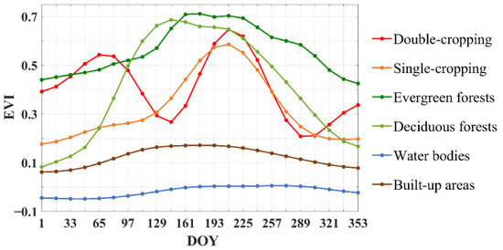
Figure 4.
EVI profiles of major land-cover types in Hubei province. A total of 3000 samples were collected to generate EVI profiles, including 537 of double-cropping, 622 single-cropping, 486 evergreen forests, 432 deciduous forests, 517 water bodies and 406 built-up areas.
Principal component analysis (PCA) has been proven to be effective at detecting seasonal changes in vegetation when applied to the time series vegetation index [44]. PCA transformation projects original data into new k-dimensional components ordered by variance, with the majority of information provided by the first several components. PCA components have geographic meanings; for example, Henderson et al. [45] found the components corresponding closely to typical vegetation density or degree of seasonality, Wang et al. [46] found the components coinciding with the average normalized difference vegetation index (NDVI) (PCA component 1) and accounting for the most prominent man-induced vegetation alterations (PCA component 2).
PCA transformation was applied to the original time series MODIS EVI to obtain components with geographic meanings while reducing feature dimensions. In this study, the first three components reserved 93.18% of the original information. From PCA component 1 (PCA 1), vegetation and non-vegetation (water bodies and built-up areas) could be easily distinguished, and the difference between natural vegetation and croplands was also very significant (Figure 5a,b). PCA component 2 (PCA 2) could discriminate double-cropping from other land-cover types, and the difference between double-cropping and single-cropping was also very obvious (Figure 5c). Moreover, PCA component 3 (PCA 3) could discriminate single-cropping from other land-cover types (Figure 5d). Therefore, the combination of the first few components could be used to discriminate the major land-cover types.
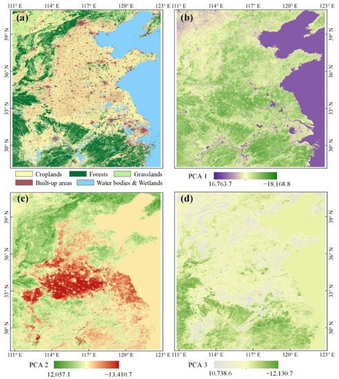
Figure 5.
Land-cover types (a) and the first three PCA components of the time series EVI, (b) PCA 1, (c) PCA 2 and (d) PCA 3.
2.2.2. Feature Space Construction and Endmember Selection
The key for the unmixing is the selection of appropriate endmembers. The accuracy of unmixing was directly affected by the quality and quantity of the selected endmembers. A triangle is the simplest simplex when the convex geometry is introduced for the unmixing [47]. Convex cone analysis takes the boundary points of the convex cone constructed from the observed spectra as the endmembers [48].
Two PCA components were employed to implement a projection from image space to feature space and visually examine the distribution of the candidate endmembers in the feature space. The combinations were from any two of the first three components. Candidate endmember land-cover classes were sourced from the major land-cover types of the study area and include natural vegetation, water bodies, double-cropping, single-cropping and built-up areas. Since the purpose of the study was to map cropping intensity, the cropland was subdivided into single-cropping and double-cropping, while other land-cover types were used in broad categories.
Through observing these combinations, four candidate endmembers were obtained: double-cropping, single-cropping, natural vegetations and water bodies (Figure 6).
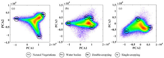
Figure 6.
The feature space and the distributions of major land-cover types with different PCA component combinations, in which the gray dots are all pixels of the images. (a) PCA 1, PCA 2 combination, (b) PCA 1, PCA 3 combination, (c) PCA 2, PCA 3 combination.
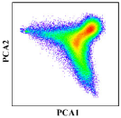
Through visually examining the scatter points based on the N-dimensional visualization tool in ENVI, we found that the PCA 1 and PCA 3 combination and PCA 2 and PCA 3 combination should be excluded, and the PCA 1 and PCA 2 combination would be the best choice (Figure 6). The mixture of single-cropping and natural vegetation could explain the exclusion of the PCA 1 and PCA 3 combination. As for the exclusion of the PCA 2 and PCA 3 combination, the single-cropping could not be used as an endmember because its cropping intensity was about half that of double-cropping theoretically and could only be inside the boundary of the feature space. With the PCA 1 and PCA 2 combination, all pixels clustered closest to a triangle in the feature space, with three vertexes representing double-cropping, natural vegetation and water bodies, which could be the candidate endmembers (Figure 7).
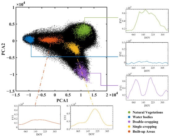
Figure 7.
The triangular feature space, in which the black dots are all pixels of the images, and the colored dots are candidate endmember land-cover types. The EVI profiles of relevant land-cover types are also presented.
We also found that single-cropping was located in the transition zone from double-cropping to the center of the feature space, and built-up areas were located in the transition zone from water bodies to the center of the feature space. Double-cropping occupied one of the corners and had the highest cropping intensity; natural vegetation and water bodies were located in the other two corners and had zero cropping intensity; single-cropping was on the transition zone from double-cropping to the center of the feature space and had decreased cropping intensity. From these analyses, the unmixing based on this triangle feature space met the requirements of our research. Therefore, three endmembers were selected finally: double-cropping, natural vegetation and water bodies.
To guarantee the purity of endmembers, the Sentinel-2 images and historical images on the Google Earth platform were used to identify large fields to assist the manual endmember collection. High accuracy can be obtained by manually selecting endmember pixels through the visual interpretation method [49]. The pure pixels corresponding to the endmembers were widely distributed across the study area, and the amount reached about 0.5% of the total pixels.
2.2.3. Cropping Intensity Estimation
The LSMA model was used to implement the TMA method. The fully constrained LSMA model was used to estimate the abundance of each endmember. The unmixing was conducted in the time dimension by replacing the original spectral information with multi-temporal vegetation indices. The linear unmixing method assumed that the EVI temporal spectra of a pixel are a linear combination of each endmember. The formulas of linear spectral unmixing (1) and constraints (2) and (3) are as follows:
where is the EVI value for each phase i in the temporal EVI image, is the number of end members, is the fraction for each end member , is the EVI value of endmember in phase (also the abundance of each endmember), and is the residual.
The abundances of all endmembers were under the constraint of being non-negative and added up to 1. The abundance of double-cropping was extracted and was regarded as cropping intensity, in which pixel value 0 represented abandoned cropland, and pixel value 1 represented homogeneous double-cropping areas.
2.2.4. Validation of the Model
In addition to visual examination, the estimated cropping intensity was validated by using the Sentinel-2 derived cropping intensity data, MCD12Q2 product, GCI dataset and GCI30 dataset as references.
The accuracy of the model output was evaluated using the coefficient of determination R2, root mean square error (RMSE) of the linear fitting with respect to the reference data.
The validation was conducted at grid level and county level, respectively. On grid level, both the modeled result and the reference data were aggregated to 2 km fractural images by summarizing the values within each grid. On county level, zonal statistics were used to summarize the data to county level for those complete counties in the research area.
The software packages used in this research for constructing the feature space and the model validation were ENVI (ENVI version 4.8, Exelis Visual Information Solutions, Boulder, CO, USA) and MATLAB (MATLAB 2018a, The MathWorks, Inc., Natick, MA, USA).
3. Results
3.1. Cropping Intensity Map
The developed TMA method was used to estimate cropping intensity in the research area in 2018 (Figure 8). Relatively high cropping intensity could be found in the North China Plain and the center and north of Hubei Province. Furthermore, natural vegetation, water bodies, and built-up areas featured very low intensity values.
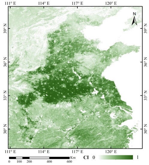
Figure 8.
Cropping intensity of the study area in 2018.
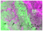
A comparison of the estimated cropping intensity with MODIS false-color composite images and cropping frequency is presented in Figure 9. Since double-cropping areas had high EVI values on DOY 065 and DOY 209 and low EVI values on DOY 145 (Figure 4), they have a magenta tone in the false-color composite images. It can be observed that the high cropping intensity pixels in the estimated cropping intensity correlate well with those magenta pixels in the MODIS image. Additionally, the estimated cropping intensity avoids dividing the cropping intensity into fixed categories like cropping frequency, and thus contains detailed information.
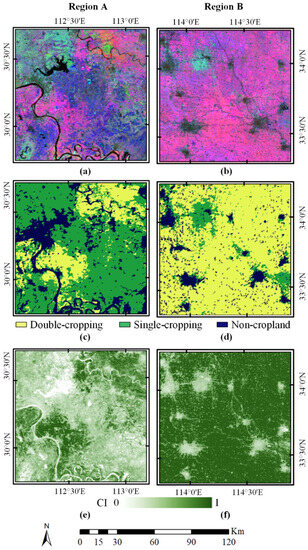
Figure 9.
Visual comparison of cropping intensity in 2018; (a,b) are MODIS false-color composites (DOY 065, 145, 225); (c,d) are cropping frequency from MCD12Q2; (e,f) are the estimated cropping intensity for the test regions A and B.
3.2. Validation Results
When using linear fitting at the grid level, 1000 cases were randomly selected to analyze the agreement between the Sentinel-2 derived cropping intensity data and the estimated cropping intensity in the two test regions. The coefficient of determination (R2) of the linear fitting reached 0.85 and 0.94 in the two test regions, respectively (Figure 10), suggesting that our cropping intensity result well captures the variations in the reference samples.
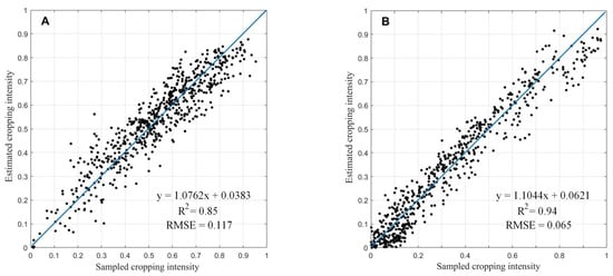
Figure 10.
Linear fitting of the Sentinel-2 derived cropping intensity and estimated cropping intensity. (A,B) are two test regions.
The agreement between the three cropping frequency datasets (MCD12Q2, GCI and GCI30) and estimated cropping intensity at the county level is presented in Figure 11. Their R2 all achieved 0.93, demonstrating that the performance of our method is satisfactory (Figure 11).
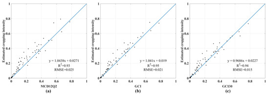
Figure 11.
Linear fitting of the estimated cropping intensity and three cropping frequency datasets at the county level: (a) MCD12Q2, (b) GCI and (c) GCI30.
4. Discussions
4.1. Determining the Final Endmembers
To demonstrate the validity of the final endmembers, three PCA components were used to visually examine the distribution of the candidate endmembers in the feature space (Figure 12). Through rotating the feature space, different PCA component combinations could be obtained and be represented in this three-dimensional space. For the two-dimensional case, it was viewed by rotating the feature space to compress one of the dimensions. It was difficult to visualize the one-dimensional case, so it was carried out in the two-dimensional space and assumed to be projected into one of the features. PCA 2 was found to be the most ideal feature when one feature was used. Table 2 lists all possible combinations using the three PCA components.
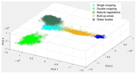
Figure 12.
The three-dimensional feature space.

Table 2.
Multiple endmember models.
Through the visual examination, we found that three models might meet our requirements (Table 2, in bold font). With the first model, it was difficult to meet the purity requirements for the endmembers because it lacked major land-cover types. The four-endmember model (the fifth model) did not fit the definition of cropping intensity in our study because single-cropping was also taken as one of the endmembers. Therefore, the three-endmember model using PCA 1 and PCA 2 was finally selected.
4.2. Delineating the Endmembers Manually
Accurate and fast endmember selection is the key to the successful application of the method. Although the endmember selection based on high-resolution remote sensing images (named ESRS) could ensure the purity and representativeness of the endmembers, it suffered from the heavy load of work for pure pixel selection and was highly dependent on the availability of high-resolution images.
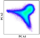
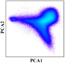
Therefore, we explored the feasibility of manually delineating endmembers (named MDE). This was achieved by drafting the vertex of the convex simplex through human–computer interaction in the feature space. We first delineated those pixels around the vertices as endmembers, as close to the vertices as possible. As this work was susceptible to the operator’s knowledge of what a “vertex” is, the operation was repeated three times by covering different area sizes (Figure 13).
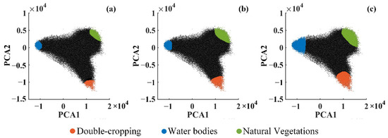
Figure 13.
Delineating endmembers with different area sizes: size 1 (a), size 2 (b), size 3 (c). The sizes of the area gradually expand.
The estimated cropping intensity with different vertex sizes was compared with MCD12Q2 at the county level. The R2 of the correlation between the estimation and MCD12Q2 were all above 0.87 (Figure 14), which confirmed that the proposed endmember selection method is applicable and robust. Compared with ESRS, MDE has the advantages of high efficiency and ease of implementation, and the accuracy and efficiency can be well-balanced.
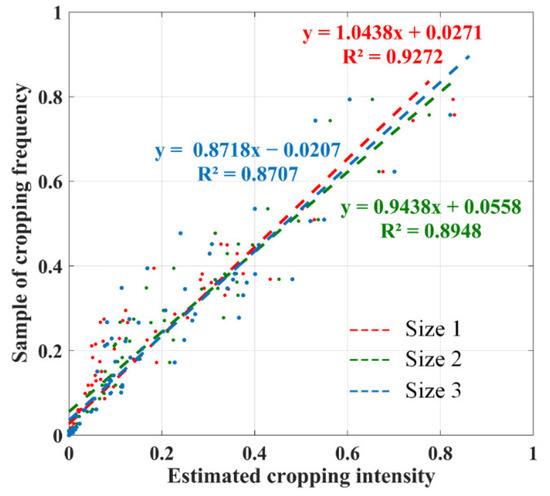
Figure 14.
Correlation between MCD12Q2 and MDE estimated at the county level.
The accuracy of the unmixing decreased slightly when the sizes of endmember areas expanded (Figure 14). This is explainable since the closer the endmember is to the vertex of the convex simplex, the purer the endmember will be. Therefore, to ensure the accuracy, the delineating area of endmembers should be as small as possible and as close to the vertex as possible.
4.3. Unmixing in Regions with Different Sizes and Varied Endmember Land-Cover Types
The shape of the feature space varied when the research area covered different regions with different sizes. The shape of the feature space affected the unmixing accuracy since the approximate triangle was the basis of the method. Therefore, the relationships of the size of the research area and the completeness of the land-cover types with the unmixing accuracies were explored.
The estimated cropping intensity and MCD12Q2 were compared for test areas with different sizes (Figure 15). The mean cropping intensity values were compared at 10 km × 10 km block level. The area sizes, the corresponding feature space and the unmixing accuracies for each test area are given in Table 3.
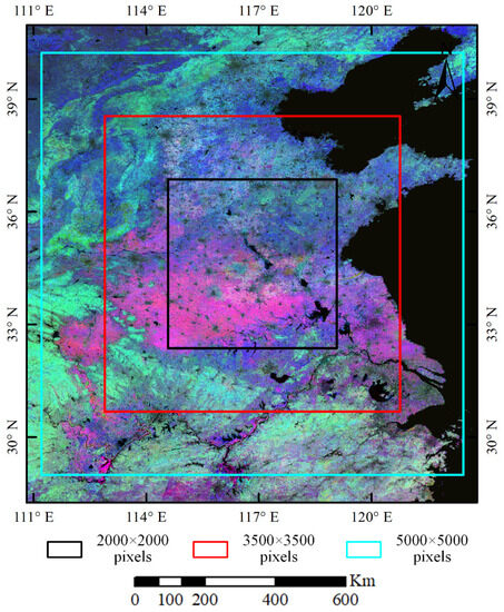
Figure 15.
Test areas with different sizes.

Table 3.
The unmixing accuracies for areas with different sizes.
The completeness of the three endmembers in the study area was the precondition for the successful application of this method. The three vertices in the feature spaces were obvious in all test areas with varied sizes. R2 values were above 0.87 in all test areas, demonstrating that the size of the study area had little effect on the unmixing accuracy as long as the study area had all necessary land-cover types.
The effectiveness of the proposed method also depends on the completeness of endmember land-cover types. Our method can be applied directedly to the North China Plain and the middle and lower reaches of the Yangtze River Valley, which are double-cropping or double-single-mixed cropping areas with relatively large patches of croplands. The successful application of the method requires the concurrence of three land-cover types (double-cropping, natural vegetation and water bodies). The method will need further work (for example, to construct a new feature space, to find the new optimal endmembers again) when lacking any of the three necessary endmember land-cover types, such as those areas where crops have only one growing season (Table 4). However, expanding the test area does aid the inclusion of all three necessary endmember land-cover types.

Table 4.
Completeness of endmembers when test areas are located in regions with varied land-cover types.
More effort is needed to find the proper endmembers when the method is extended to areas other than China. Since the interpretation for PCA images is scene-dependent and there has been no well outlined procedure for it, the interpretation needs more elaboration, and that is where innovation is possible.
The abundance of natural vegetation and water bodies can also be estimated as a “by-product” of this research. MODIS MOD13Q1 products within a year were used and the focus was cropping intensity estimation in this study. If the method is transplanted to time series vegetation indices with different temporal spans, other land-cover types can also be unmixed.
5. Conclusions
Fine cropping intensity mapping is essential for agricultural production and the sustainable development of agriculture. This study reports our work on developing a new method to estimate cropping intensity from time series remote sensing data for a specific region of China. A novel feature space was constructed, and three unique endmembers (double-cropping, natural vegetation and water bodies) were found. A new TMA method was developed to map cropping intensity at the abundance level. The estimated results were compared with sample data and cropping intensity product data at the pixel and county levels, respectively. The experiments demonstrated that the method is a highly accurate, semi-automatic, and easily implemented approach suitable for large-scale and long time-series cropping intensity mapping.
The study provided a novel method for cropping intensity estimation from historical archived time-series coarse-resolution remote sensing data. Firstly, a new TMA method was developed to conduct spatio-temporal continuous fine-resolution cropping intensity mapping from coarse-resolution remote sensing data. The phenology information was fully mined considering the seasonal variation in vegetation, including the phenological difference between crops and other land-cover types. Secondly, a unique feature space was constructed, along with three endmembers: double-cropping, natural vegetation and water bodies. The estimated results expressed crop extent and cropping intensity at the abundance level, improving the precision of cropping intensity estimation and avoiding dividing crop patterns rigidly into double-cropping or single-cropping. Thirdly, the MDE method has the advantage of high efficiency and ease of implementation, facilitating the endmember selection and unmixing process. The research provided insights into TMA-based cropping intensity mapping.
Future work will involve extending the method to a wider area and discussing the impact of regional differentiation on the unmixing accuracy.
Author Contributions
Conceptualization, J.T.; Methodology, J.T.; Validation, X.Z. and Q.J.; Data curation, X.Z. and Y.L.; Writing—original draft, Y.L.; Writing—review & editing, Y.Z. All authors have read and agreed to the published version of the manuscript.
Funding
This work was supported by the National Natural Science Foundation of China (Grant No. 41971371 and 32001368), the National Key Technologies Research and Development Program (Grant No. 2022YFB3903504) and the Fundamental Research Funds for the Central Universities (CCNU22JC022).
Data Availability Statement
No new data were created or analyzed in this study. Data sharing is not applicable to this article.
Acknowledgments
The authors appreciate the comments and suggestions from anonymous reviewers.
Conflicts of Interest
The authors declare no conflict of interest.
References
- Zhu, H.; Sun, M. Main progress in the research on land use intensification. Acta Geogr. Sin. 2014, 69, 1346–1357. [Google Scholar]
- Liu, G.; Zhang, L.; Zhang, Q.; Musyimi, Z. The response of grain production to changes in quantity and quality of cropland in yangtze river delta, China. J. Sci. Food Agric. 2015, 95, 480–489. [Google Scholar] [CrossRef]
- Liu, J.; Kuang, W.; Zhang, Z.; Xu, X.; Qin, Y.; Ning, J.; Zhou, W.; Zhang, S.; Li, R.; Yan, C.; et al. Spatiotemporal characteristics, patterns, and causes of land-use changes in China since the late 1980s. J. Geogr. Sci. 2014, 24, 195–210. [Google Scholar] [CrossRef]
- Tao, J.; Wang, Y.; Qiu, B.; Wu, W. Exploring cropping intensity dynamics by integrating crop phenology information using bayesian networks. Comput. Electron. Agric. 2022, 193, 106667. [Google Scholar] [CrossRef]
- Su, Y.; Qian, K.; Lin, L.; Wang, K.; Guan, T.; Gan, M. Identifying the driving forces of non-grain production expansion in rural China and its implications for policies on cultivated land protection. Land Use Policy 2020, 92, 104435. [Google Scholar] [CrossRef]
- Liu, X.; Herbert, S.J. Fifteen years of research examining cultivation of continuous soybean in northeast China: A review. Field Crops Res. 2002, 79, 1–7. [Google Scholar] [CrossRef]
- Sun, J.; Mooney, H.; Wu, W.; Tang, H.; Tong, Y.; Xu, Z.; Huang, B.; Cheng, Y.; Yang, X.; Wei, D.; et al. Importing food damages domestic environment: Evidence from global soybean trade. Proc. Natl. Acad. Sci. USA 2018, 115, 5415–5419. [Google Scholar] [CrossRef]
- Li, S.; Li, X.; Sun, L.; Cao, G.; Fischer, G.; Tramberend, S. An estimation of the extent of cropland abandonment in mountainous regions of China. Land Degrad. Dev. 2018, 29, 1327–1342. [Google Scholar] [CrossRef]
- Peng, W.; Ma, N.L.; Zhang, D.; Zhou, Q.; Yue, X.; Khoo, S.C.; Yang, H.; Guan, R.; Chen, H.; Zhang, X. A review of historical and recent locust outbreaks: Links to global warming, food security and mitigation strategies. Environ. Res. 2020, 191, 110046. [Google Scholar] [CrossRef]
- Mottaleb, K.A.; Kruseman, G.; Snapp, S. Potential impacts of ukraine-russia armed conflict on global wheat food security: A quantitative exploration. Glob. Food Secur. 2022, 35, 100659. [Google Scholar] [CrossRef]
- Rahimi, P.; Islam, M.S.; Duarte, P.M.; Tazerji, S.S.; Sobur, M.A.; El Zowalaty, M.E.; Ashour, H.M.; Rahman, M.T. Impact of the COVID-19 pandemic on food production and animal health. Trends Food Sci. Technol. 2022, 121, 105–113. [Google Scholar] [CrossRef] [PubMed]
- Yu, X.; Liu, C.; Wang, H.; Feil, J.-H. The impact of COVID-19 on food prices in China: Evidence of four major food products from beijing, shandong and hubei provinces. China Agric. Econ. Rev. 2020, 12, 445–458. [Google Scholar] [CrossRef]
- Dongyu, Q. Role and Potential of Potato in Global Food Security; FAO: Rome, Italy, 2022. [Google Scholar]
- Liu, W.; Yang, H.; Liu, Y.; Kummu, M.; Hoekstra, A.Y.; Liu, J.; Schulin, R. Water resources conservation and nitrogen pollution reduction under global food trade and agricultural intensification. Sci. Total Environ. 2018, 633, 1591–1601. [Google Scholar] [CrossRef] [PubMed]
- Rachele, R. Briefing-Desertification and Agriculture; European Parliament: Strasbourg, France, 2020. [Google Scholar]
- Xu, B.; Niu, Y.; Zhang, Y.; Chen, Z.; Zhang, L. China’s agricultural non-point source pollution and green growth: Interaction and spatial spillover. Environ. Sci. Pollut. Res. 2022, 29, 60278–60288. [Google Scholar] [CrossRef] [PubMed]
- Liu, Y.; Tang, H.; Muhammad, A.; Huang, G. Emission mechanism and reduction countermeasures of agricultural greenhouse gases—A review. Greenh. Gases Sci. Technol. 2019, 9, 160–174. [Google Scholar] [CrossRef]
- Xie, H.; Liu, G. Spatiotemporal difference and determinants of multiple cropping index in China during 1998–2012. Acta Geogr. Sin. 2015, 70, 604–614. [Google Scholar]
- Guo, Y.; Xia, H.; Pan, L.; Zhao, X.; Li, R. Mapping the northern limit of double cropping using a phenology-based algorithm and google earth engine. Remote Sens. 2022, 14, 1004. [Google Scholar] [CrossRef]
- Jiang, M.; Xin, L.; Li, X.; Tan, M.; Wang, R. Decreasing rice cropping intensity in southern China from 1990 to 2015. Remote Sens. 2019, 11, 35. [Google Scholar] [CrossRef]
- Löw, F.; Biradar, C.; Dubovyk, O.; Fliemann, E.; Akramkhanov, A.; Narvaez Vallejo, A.; Waldner, F. Regional-scale monitoring of cropland intensity and productivity with multi-source satellite image time series. Gisci. Remote Sens. 2018, 55, 539–567. [Google Scholar] [CrossRef]
- Qiu, B.; Lu, D.; Tang, Z.; Song, D.; Zeng, Y.; Wang, Z.; Chen, C.; Chen, N.; Huang, H.; Xu, W. Mapping cropping intensity trends in China during 1982–2013. Appl. Geogr. 2017, 79, 212–222. [Google Scholar] [CrossRef]
- Yan, H.; Liu, F.; Qin, Y.; Doughty, R.; Xiao, X. Tracking the spatio-temporal change of cropping intensity in China during 2000–2015. Environ. Res. Lett. 2019, 14, 035008. [Google Scholar] [CrossRef]
- Pan, L.; Xia, H.; Yang, J.; Niu, W.; Qin, Y. Mapping cropping intensity in huaihe basin using phenology algorithm, all sentinel-2 and landsat images in google earth engine. Int. J. Appl. Earth Obs. Geoinf. 2021, 102, 102376. [Google Scholar] [CrossRef]
- Liu, L.; Xiao, X.; Qin, Y.; Wang, J.; Xu, X.; Hu, Y.; Qiao, Z. Mapping cropping intensity in China using time series landsat and sentinel-2 images and google earth engine. Remote Sens. Environ. 2020, 239, 111624. [Google Scholar] [CrossRef]
- Liu, C.; Zhang, Q.; Tao, S.; Qi, J.; Ding, M.; Guan, Q.; Wu, B.; Zhang, M.; Nabil, M.; Tian, F. A new framework to map fine resolution cropping intensity across the globe: Algorithm, validation, and implication. Remote Sens. Environ. 2020, 251, 112095. [Google Scholar] [CrossRef]
- Tao, J.; Wu, W.; Xu, M. Using the bayesian network to map large-scale cropping intensity by fusing multi-source data. Remote Sens. 2019, 11, 168. [Google Scholar] [CrossRef]
- Tao, J.; Wu, W.; Liu, W. Spatial-temporal dynamics of cropping frequency in hubei province over 2001–2015. Sensors 2017, 17, 2622. [Google Scholar] [CrossRef]
- Qiu, B.; Li, W.; Tang, Z.; Chen, C.; Qi, W. Mapping paddy rice areas based on vegetation phenology and surface moisture conditions. Ecol. Indic. 2015, 56, 79–86. [Google Scholar] [CrossRef]
- Tian, H.F.; Huang, N.; Niu, Z.; Qin, Y.C.; Pei, J.; Wang, J. Mapping winter crops in China with multi-source satellite imagery and phenology-based algorithm. Remote Sens. 2019, 11, 820. [Google Scholar] [CrossRef]
- d’Andrimont, R.; Taymans, M.; Lemoine, G.; Ceglar, A.; Yordanov, M.; van der Velde, M. Detecting flowering phenology in oil seed rape parcels with sentinel-1 and-2 time series. Remote Sens. Environ. 2020, 239, 111660. [Google Scholar] [CrossRef]
- Pok, S.; Matsushita, B.; Fukushima, T. An easily implemented method to estimate impervious surface area on a large scale from modis time-series and improved dmsp-ols nighttime light data. ISPRS J. Photogramm. Remote Sens. 2017, 133, 104–115. [Google Scholar] [CrossRef]
- Chen, Y.; Yun, W.; Zhou, X.; Peng, J.; Li, S.; Zhou, Y. Classification and extraction of land use information in hilly area based on mesma and rf classifier. Trans. Chin. Soc. Agric. Mach 2017, 48, 136–144. [Google Scholar]
- Ridd, M.K. Exploring a vis (vegetation-impervious surface-soil) model for urban ecosystem analysis through remote sensing: Comparative anatomy for cities. Int. J. Remote Sens. 1995, 16, 2165–2185. [Google Scholar] [CrossRef]
- Ji, C.; Li, X.; Wei, H.; Li, S. Comparison of different multispectral sensors for photosynthetic and non-photosynthetic vegetation-fraction retrieval. Remote Sens. 2020, 12, 115. [Google Scholar] [CrossRef]
- Pi, X.; Zeng, Y.; He, C. High-resolution urban vegetation coverage estimation based on multi-source remote sensing data fusion. Natl. Remote Sens. Bull. 2021, 25, 1216–1226. [Google Scholar] [CrossRef]
- Wang, Y.; Zhuo, R.; Xu, L.; Fang, Y. A spatial-temporal bayesian deep image prior model for moderate resolution imaging spectroradiometer temporal mixture analysis. Remote Sens. 2023, 15, 3782. [Google Scholar] [CrossRef]
- Caballero, I.; Stumpf, R.P. Towards routine mapping of shallow bathymetry in environments with variable turbidity: Contribution of sentinel-2a/b satellites mission. Remote Sens. 2020, 12, 451. [Google Scholar] [CrossRef]
- Gray, J.; Sulla-Menashe, D.; Friedl, M.A. User Guide to Collection 6 Modis Land Cover Dynamics (mcd12q2) Product. In NASA EOSDIS Land Process; DAAC: Missoula, MT, USA, 2019; Volume 6, pp. 1–8. [Google Scholar]
- Liu, X.; Zheng, J.; Yu, L.; Hao, P.; Chen, B.; Xin, Q.; Fu, H.; Gong, P. Annual dynamic dataset of global cropping intensity from 2001 to 2019. Sci. Data 2021, 8, 283. [Google Scholar] [CrossRef]
- Zhang, M.; Wu, B.; Zeng, H.; He, G.; Liu, C.; Tao, S.; Zhang, Q.; Nabil, M.; Tian, F.; Bofana, J. Gci30: A global dataset of 30 m cropping intensity using multisource remote sensing imagery. Earth Syst. Sci. Data 2021, 13, 4799–4817. [Google Scholar] [CrossRef]
- Boardman, J.W. Automated Spectral Unmixing of Aviris Data Using Convex Geometry Concepts. In Proceedings of the Jplairborne Geoscience Workshop, Washington, DC, USA, 25–29 October 1993. [Google Scholar]
- Melaas, E.K.; Friedl, M.A.; Zhu, Z. Detecting interannual variation in deciduous broadleaf forest phenology using landsat tm/etm+ data. Remote Sens. Environ. 2013, 132, 176–185. [Google Scholar] [CrossRef]
- Bellón, B.; Bégué, A.; Seen, D.L.; Almeida, C.A.d.; Simões, M. A remote sensing approach for regional-scale mapping of agricultural land-use systems based on ndvi time series. Remote Sens. 2017, 9, 600. [Google Scholar] [CrossRef]
- Henderson, C.; Petersen, K.; Redak, R. Spatial and temporal patterns in the seed bank and vegetation of a desert grassland community. J. Ecol. 1988, 76, 717–728. [Google Scholar] [CrossRef]
- Wang, T.; Kou, X.; Xiong, Y.; Mou, P.; Wu, J.; Ge, J. Temporal and spatial patterns of ndvi and their relationship to precipitation in the loess plateau of China. Int. J. Remote Sens. 2010, 31, 1943–1958. [Google Scholar] [CrossRef]
- Yang, C.; Wu, G.; Ding, K.; Shi, T.; Li, Q.; Wang, J. Improving land use/land cover classification by integrating pixel unmixing and decision tree methods. Remote Sens. 2017, 9, 1222. [Google Scholar] [CrossRef]
- Singh, R.; Kumar, V. Evaluating automated endmember extraction for classifying hyperspectral data and deriving spectral parameters for monitoring forest vegetation health. Environ. Monit. Assess. 2022, 195, 72. [Google Scholar] [CrossRef]
- Wang, H.; Wu, B.; Li, X.; Lu, S. Extraction of impervious surface in hai basin using remote sensing. J. Remote Sens. 2011, 15, 388–400. (In Chinese) [Google Scholar]
Disclaimer/Publisher’s Note: The statements, opinions and data contained in all publications are solely those of the individual author(s) and contributor(s) and not of MDPI and/or the editor(s). MDPI and/or the editor(s) disclaim responsibility for any injury to people or property resulting from any ideas, methods, instructions or products referred to in the content. |
© 2023 by the authors. Licensee MDPI, Basel, Switzerland. This article is an open access article distributed under the terms and conditions of the Creative Commons Attribution (CC BY) license (https://creativecommons.org/licenses/by/4.0/).
