


Integrated Spatial Analysis of Forest Fire Susceptibility in the Indian Western Himalayas (IWH) Using Remote Sensing and GIS-Based Fuzzy AHP Approach

 ,
,  , ,
, ,  ,
,  ,
,  ,
,
Abstract
:
1. Introduction
2. Materials and Methods
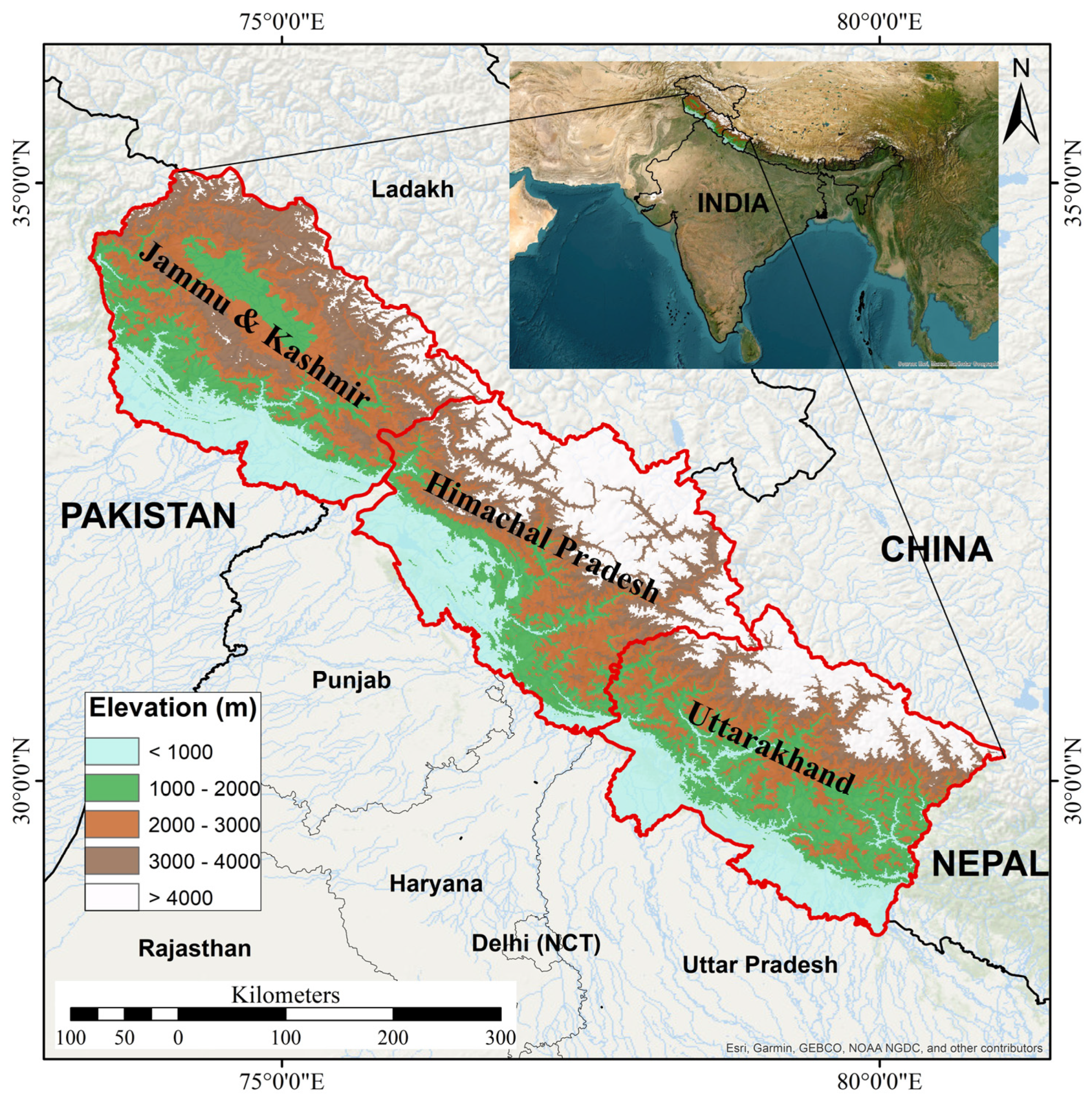
2.1. Study Area
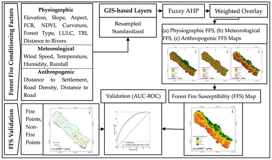
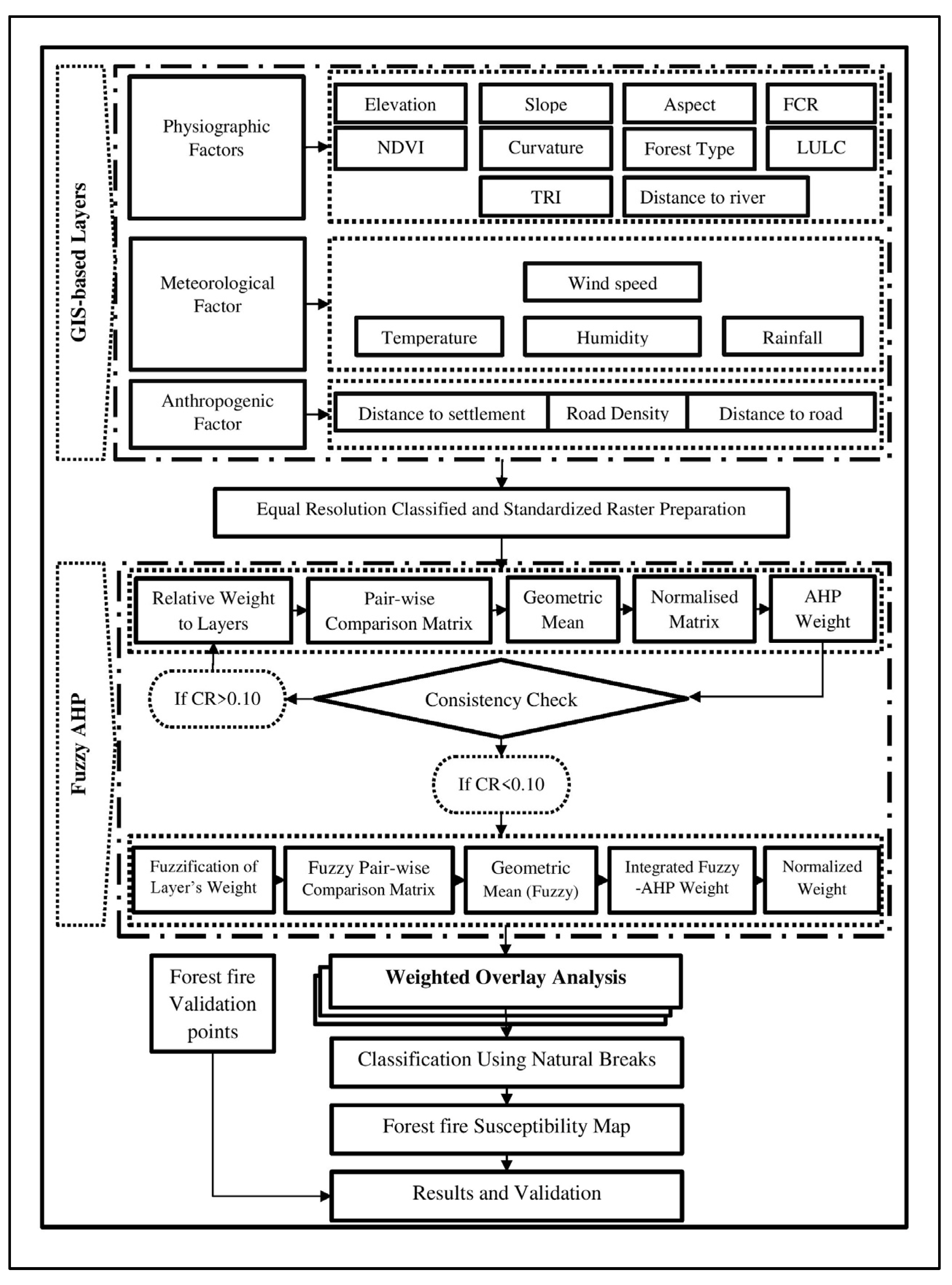
2.2. Methodology
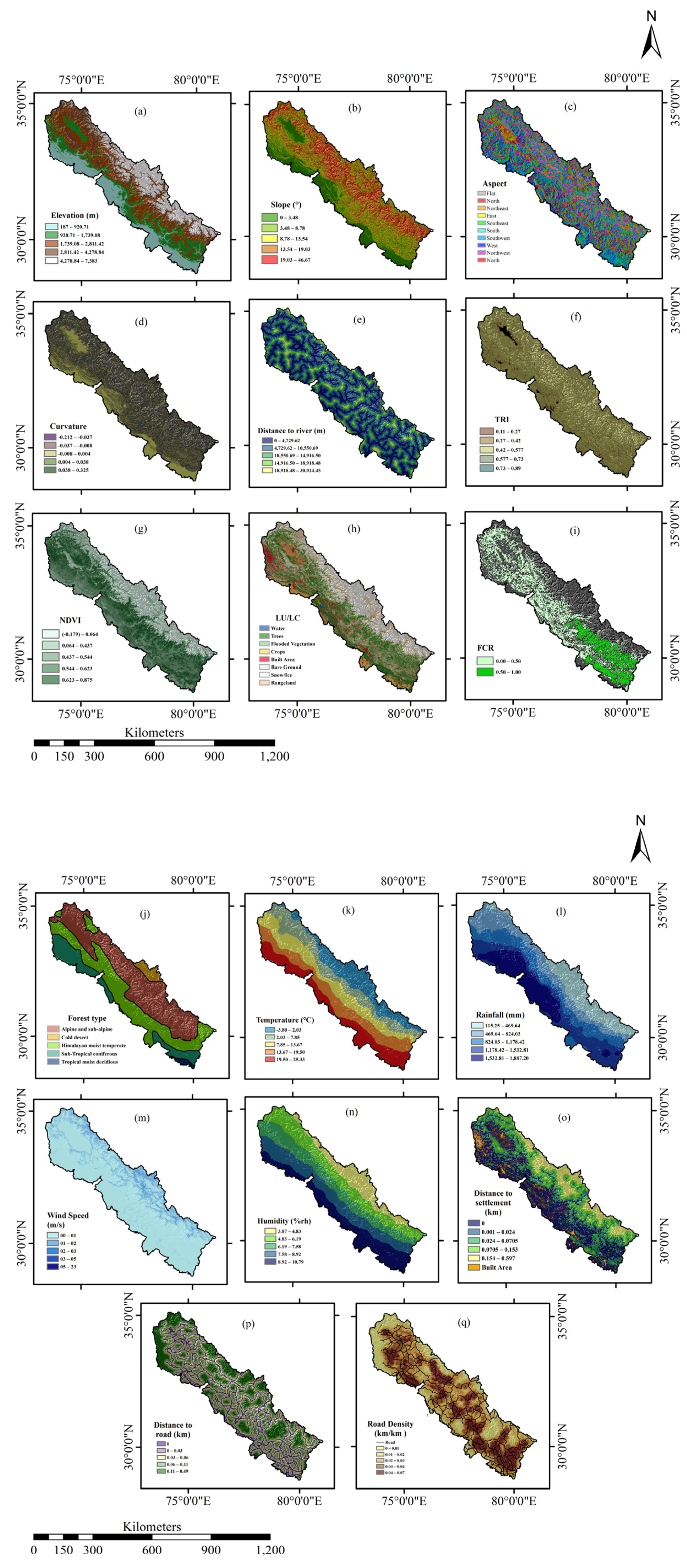
2.2.1. Forest Fire Driving Forces
Physiographic Factors
- Elevation
- Slope
- Aspect
- Curvature
- Distance to River
- Topographic Roughness Index (TRI)
- NDVI
- Land Use/Land Cover (LULC)
- Forest Coverage Ratio (FCR)
- Forest Types
Meteorological Factors
- Temperature
- Rainfall
- Wind Speed
- Humidity
Anthropogenic Factors
- Distance to Settlement
- Distance to Road
- Road Density
2.2.2. GIS-Based Fuzzy Analytical Hierarchy Process (Fuzzy-AHP) Approach
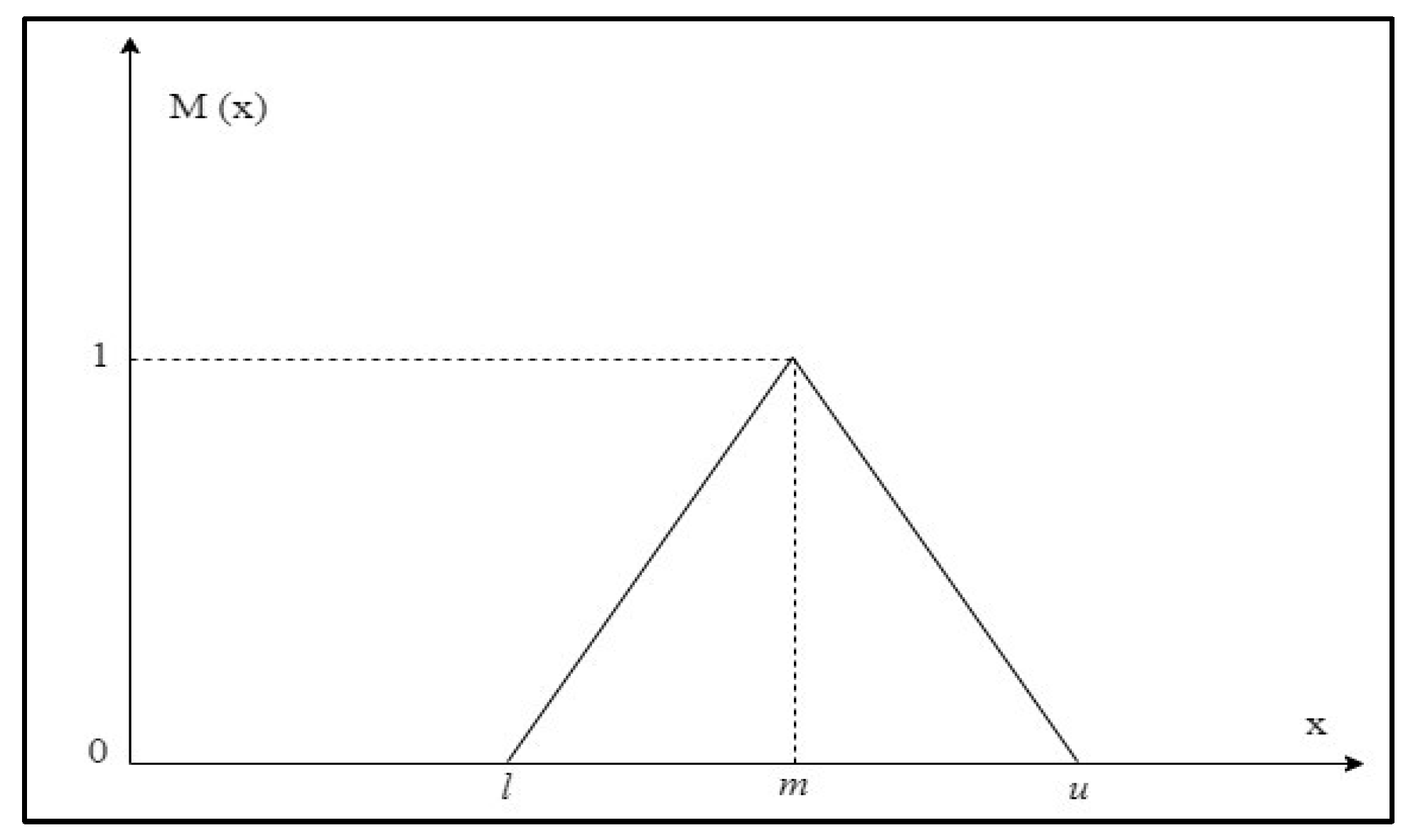
Mathematical Definitions of Fuzzy Numbers and Membership Function
Geometric Mean—Fuzzy-AHP Method
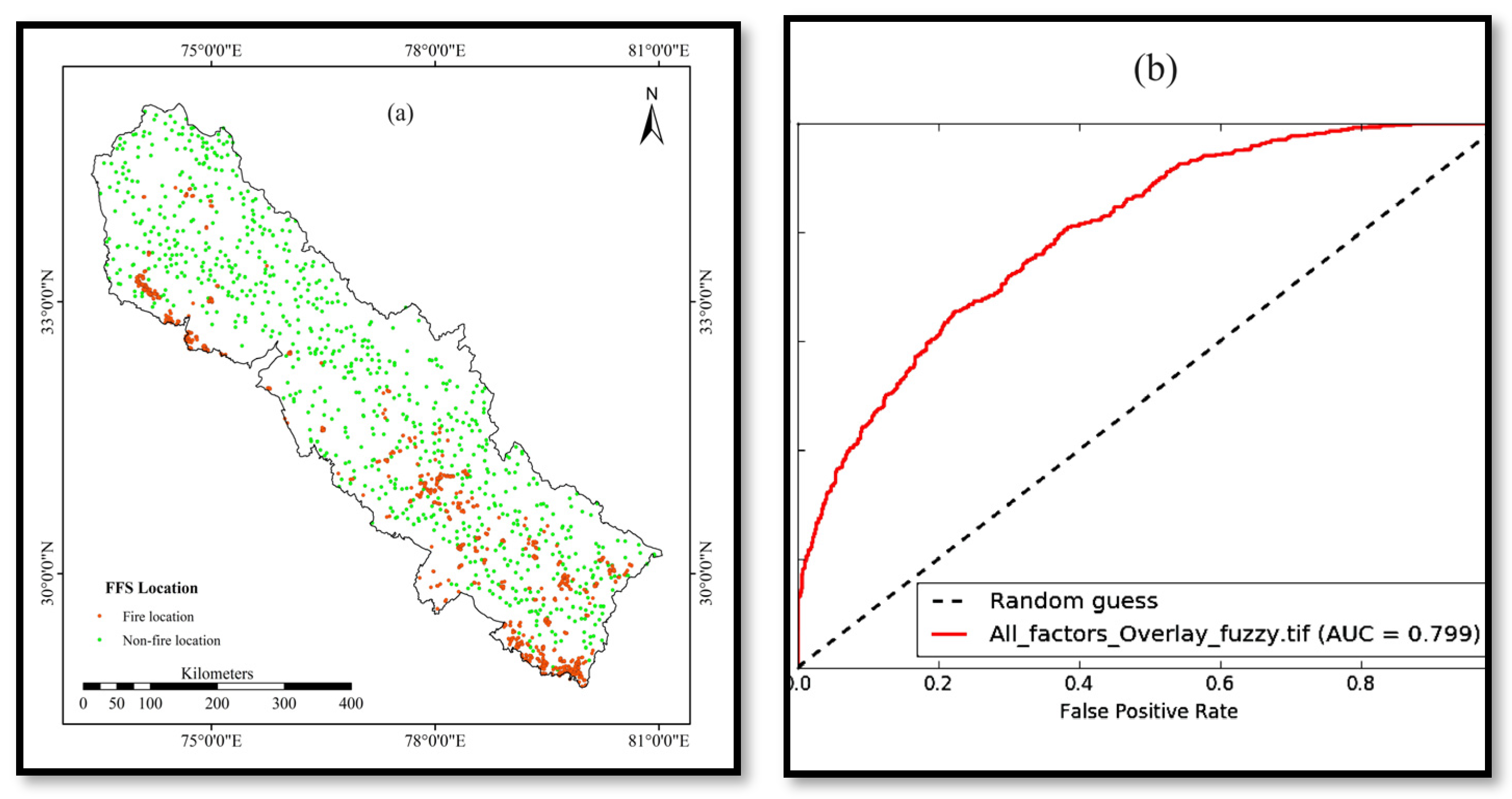
2.2.3. Validation of Forest Fire Susceptibility Maps
3. Results
3.1. Preparation of the Spatial Databases
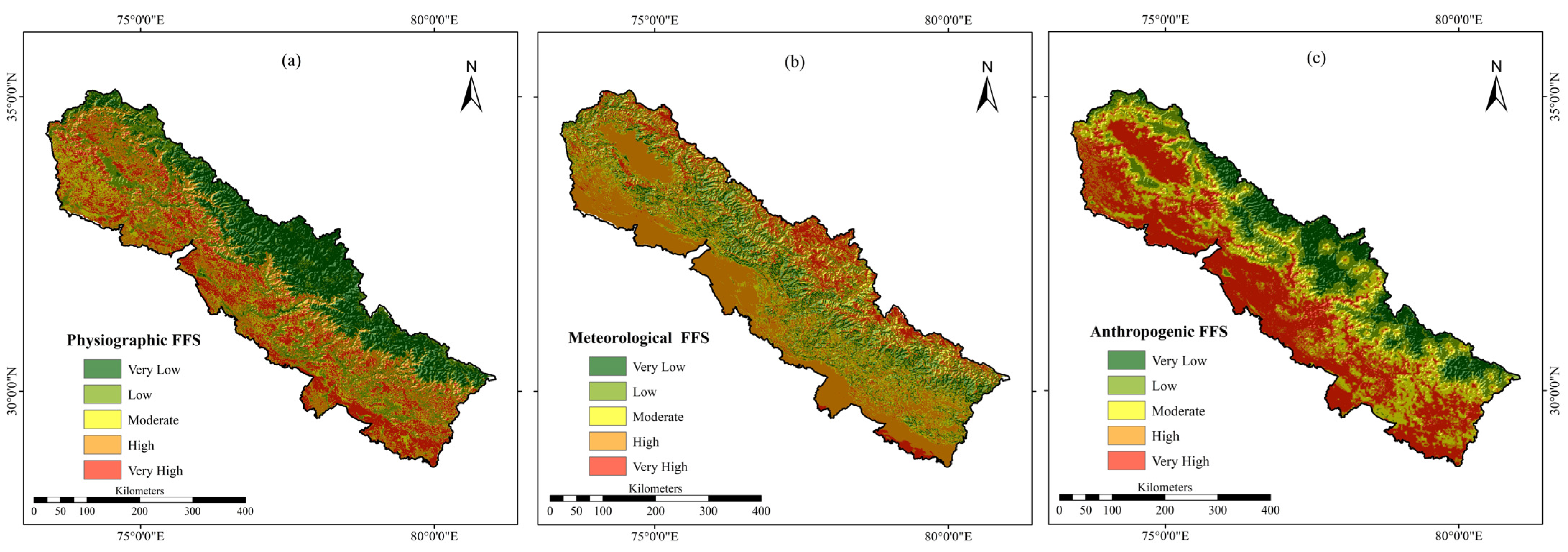
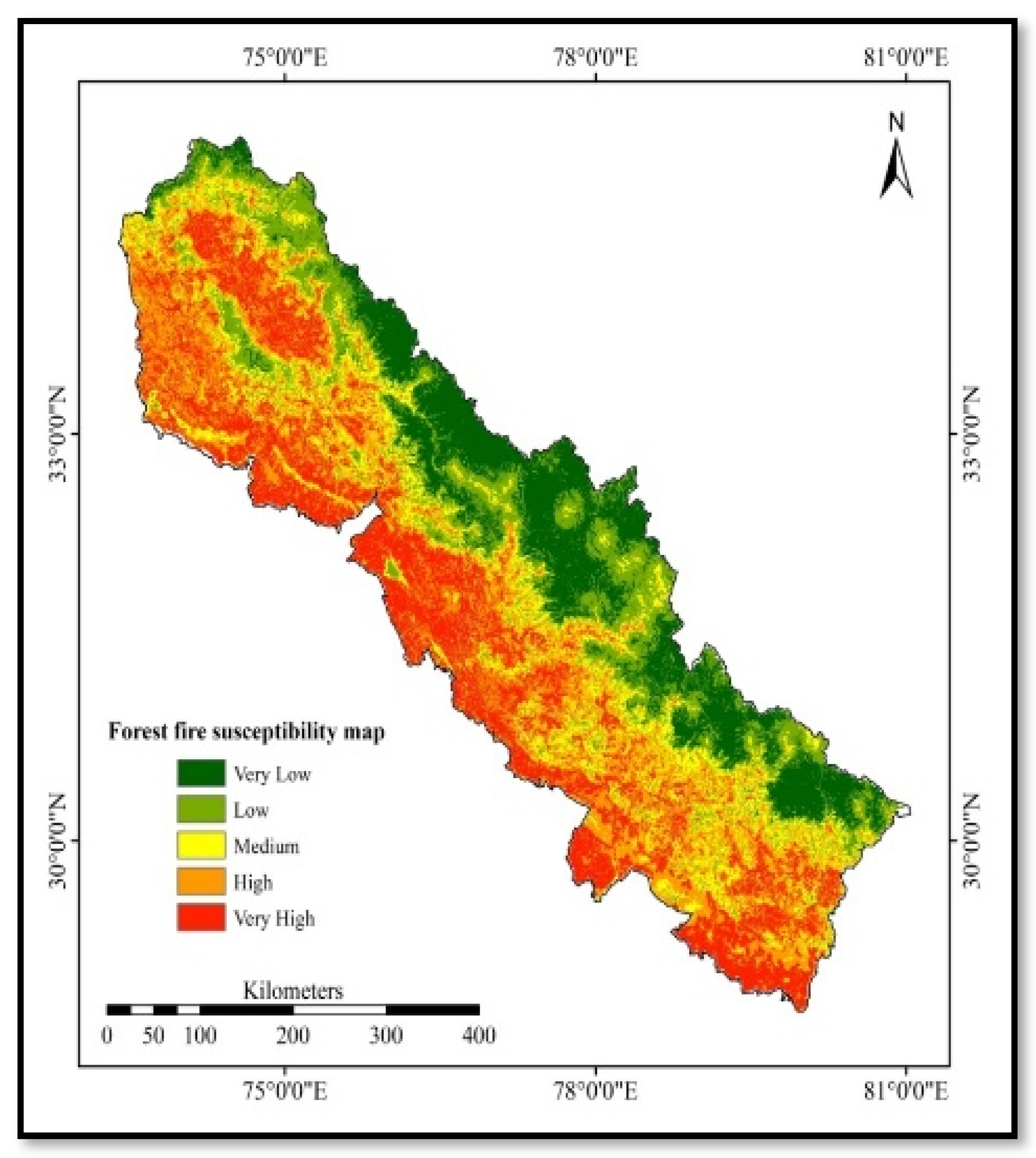
3.2. Forest Fire Susceptibility (FFS) Mapping
3.3. Map Validation Using ROC-AUC
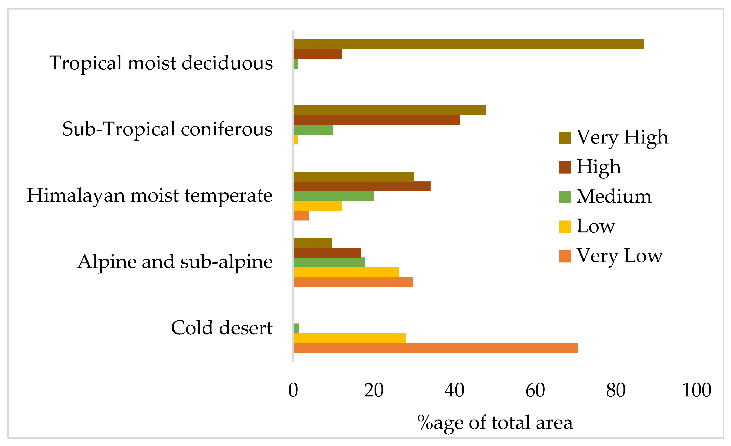
3.4. Analysis of the Vulnerability to Forest Fires by Forest Type
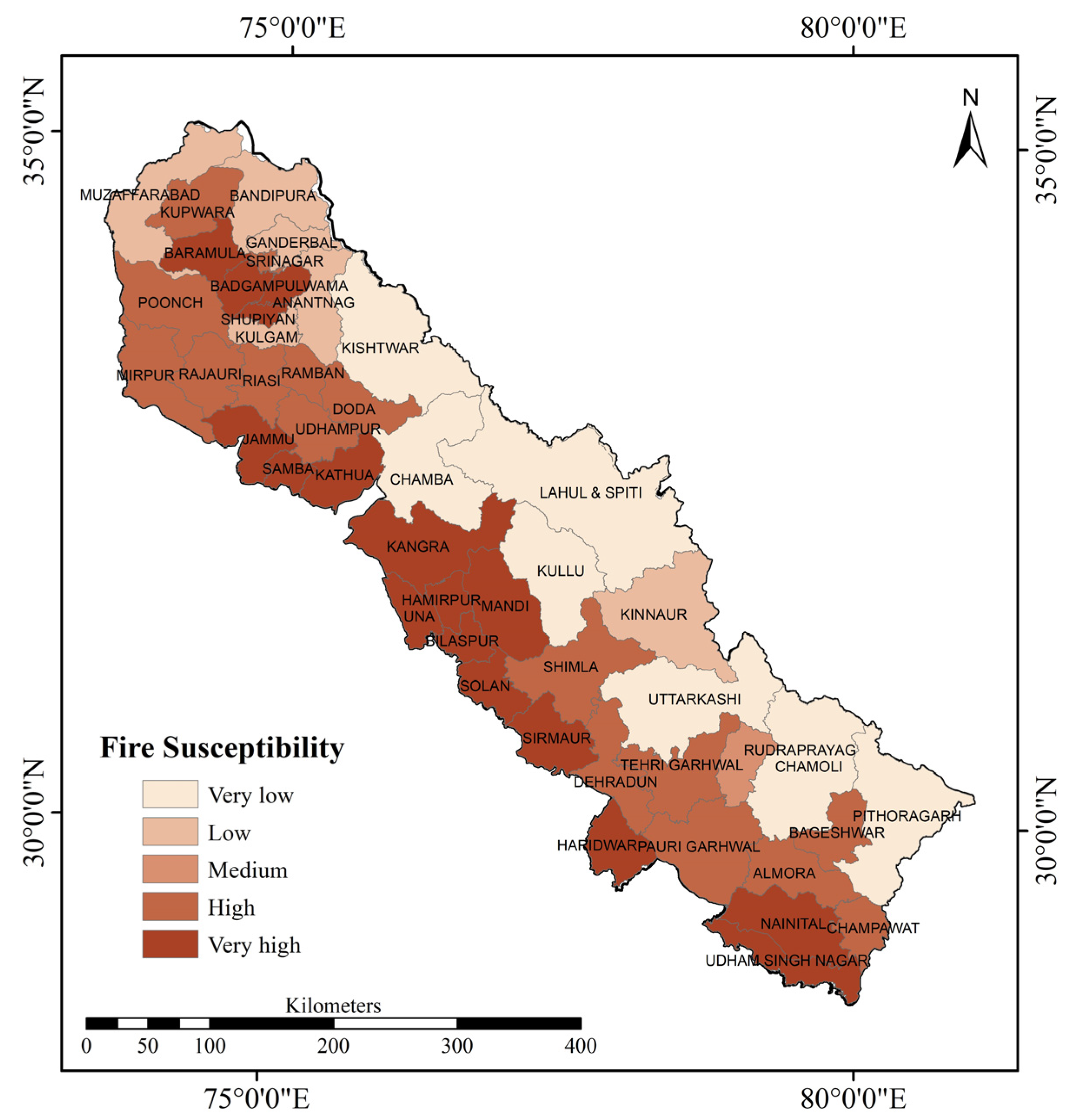
3.5. District-Wise Analysis of FFS
4. Discussion
5. Conclusions
- The IWH region has significant susceptibility to forest fire as nearly 50% area of the region is characterized as a high or very high FFS zone.
- The incidence of forest fire is specific to the forest types in the IWH region. The higher susceptibility is associated with the subtropical coniferous forests and tropical moist deciduous forests owing to the dominance of the relatively more flammable Chir pine species, in addition to the higher FCR.
- The forest fire incidence is regulated majorly by elevation, temperature, and moisture conditions in the region, and by nearness to the settlements and the roads in the IWH region.
Author Contributions
Funding
Data Availability Statement
Acknowledgments
Conflicts of Interest
References
- Gheshlaghi, H.A.; Feizizadeh, B.; Blaschke, T. GIS-based forest fire risk mapping using the analytical network process and fuzzy logic. J. Environ. Plan. Manag. 2019, 63, 481–499. [Google Scholar] [CrossRef]
- Mafi-Gholami, D.; Jaafari, A.; Zenner, E.K.; Kamari, A.N.; Bui, D.T. Spatial modeling of exposure of mangrove ecosystems to multiple environmental hazards. Sci. Total Environ. 2020, 740, 140167. [Google Scholar] [CrossRef] [PubMed]
- Nuthammachot, N.; Stratoulias, D. A GIS- and AHP-based approach to map fire risk: A case study of Kuan Kreng peat swamp forest, Thailand. Geocarto Int. 2019, 36, 212–225. [Google Scholar] [CrossRef]
- Tuyen, T.T.; Jaafari, A.; Yen, H.P.H.; Nguyen-Thoi, T.; Van Phong, T.; Nguyen, H.D.; Van Le, H.; Phuong, T.T.M.; Nguyen, S.H.; Prakash, I.; et al. Mapping forest fire susceptibility using spatially explicit ensemble models based on the locally weighted learning algorithm. Ecol. Inform. 2021, 63, 101292. [Google Scholar] [CrossRef]
- Giglio, L.; Boschetti, L.; Roy, D.P.; Humber, M.L.; Justice, C.O. The Collection 6 MODIS burned area mapping algorithm and product. Remote Sens. Environ. 2018, 217, 72–85. [Google Scholar] [CrossRef]
- Jaafari, A.; Mafi-Gholami, D.; Pham, B.T.; Tien Bui, D. Wildfire Probability Mapping: Bivariate vs. Multivariate Statistics. Remote Sens. 2019, 11, 618. [Google Scholar] [CrossRef]
- Ridder, R.M. Global forest resources assessment 2010: Options and recommendations for a global remote sensing survey of forests. In Global Remote Sensing Survey of Forests; FAO: Rome, Italy, 2007; Volume 141. [Google Scholar]
- Jain, P.; Coogan, S.C.P.; Subramanian, S.G.; Crowley, M.; Taylor, S.W.; Flannigan, M.D. A review of machine learning applications in wildfire science and management. Environ. Rev. 2020, 28, 478–505. [Google Scholar] [CrossRef]
- Tariq, A.; Shu, H.; Siddiqui, S.; Mousa, B.G.; Munir, I.; Nasri, A.; Waqas, H.; Lu, L.; Baqa, M.F. Forest fire monitoring using spatial-statistical and Geo-spatial analysis of factors determining forest fire in Margalla Hills, Islamabad, Pakistan. Geomat. Nat. Hazards Risk 2021, 12, 1212–1233. [Google Scholar] [CrossRef]
- Hansen, M.C.; Potapov, P.V.; Moore, R.; Hancher, M.; Turubanova, S.A.; Tyukavina, A.; Thau, D.; Stehman, S.V.; Goetz, S.J.; Loveland, T.R.; et al. High-resolution global maps of 21st-century forest cover change. Science 2013, 342, 850–853. [Google Scholar] [CrossRef]
- Reddy, C.S.; Bird, N.G.; Sreelakshmi, S.; Manikandan, T.M.; Asra, M.; Krishna, P.H.; Jha, C.S.; Rao, P.V.N.; Diwakar, P.G. Identification and characterization of spatio-temporal hotspots of forest fires in South Asia. Environ. Monit. Assess. 2019, 191, 1–17. [Google Scholar] [CrossRef]
- Mohanty, A.; Vidur, M. Managing Forest Fires in a Changing Climate; Council on Energy, Environment and Water: New Delhi, India, 2022. [Google Scholar]
- Bar, S.; Parida, B.R.; Pandey, A.C.; Shankar, B.U.; Kumar, P.; Panda, S.K.; Behera, M.D. Modeling and prediction of fire occurrences along an elevational gradient in Western Himalayas. Appl. Geogr. 2023, 151, 102867. [Google Scholar] [CrossRef]
- Srivastava, P.; Garg, A. Forest Fires in India: Regional and Temporal Analyses. J. Trop. For. Sci. 2013, 25, 228–239. [Google Scholar]
- Vadrevu, K.P.; Lasko, K.; Giglio, L.; Schroeder, W.; Biswas, S.; Justice, C. Trends in Vegetation fires in South and Southeast Asian Countries. Sci. Rep. 2019, 9, 7422. [Google Scholar] [CrossRef] [PubMed]
- Kumar, S.; Chaudhary, C.; Biswas, T.; Ghosh, S.; Ashutosh, S. Identification of Fire Prone Forest Areas Based on GIS Analysis of Archived Forest Fire Points Detected in Last Thirteen Years; Ministry of Environment, Forest & Climate Change, Government of India: Dehradun, India, 2019; Volume 1.
- Kumar, M. Forestry Policies and Practices to Promote Climate Change Adaptation in the Indian Western Himalayan States. In Climate Change Adaptation, Risk Management and Sustainable Practices in the Himalaya; Sharma, S., Kuniyal, J.C., Chand, P., Singh, P., Eds.; Springer International Publishing: Cham, Switzerland, 2023; pp. 65–87. [Google Scholar] [CrossRef]
- Chakraborty, A.; Joshi, P. Mapping disaster vulnerability in India using analytical hierarchy process. Geomat. Nat. Hazards Risk 2014, 7, 308–325. [Google Scholar] [CrossRef]
- Babu, K.V.S.; Roy, A.; Prasad, P.R. Forest fire risk modeling in Uttarakhand Himalaya using TERRA satellite datasets. Eur. J. Remote Sens. 2016, 49, 381–395. [Google Scholar] [CrossRef]
- Bhattarai, N.; Dahal, S.; Thapa, S.; Pradhananga, S.; Karky, B.S.; Rawat, R.S.; Windhorst, K.; Watanabe, T.; Thapa, R.B.; Avtar, R. Forest fire in the hindu kush Himalayas: A major challenge for climate action. J. For. Livelihood 2022, 21, 14–31. [Google Scholar] [CrossRef]
- Bar, S.; Parida, B.R.; Roberts, G.; Pandey, A.C.; Acharya, P.; Dash, J. Spatio-temporal characterization of landscape fire in relation to anthropogenic activity and climatic variability over the Western Himalaya, India. GIScience Remote Sens. 2021, 58, 281–299. [Google Scholar] [CrossRef]
- Tian, X.; Zhao, F.; Shu, L.; Wang, M. Distribution characteristics and the influence factors of forest fires in China. For. Ecol. Manag. 2013, 310, 460–467. [Google Scholar] [CrossRef]
- Key, C.; Benson, N. Landscape assessment: Remote sensing of severity, the normalized burn ratio and ground measure of severity, the composite burn index. In Fire Effects Monitoring and Inventory System; USDA Forest Service, Rocky Mountain Research Station: Ogden, UT, USA, 2005. [Google Scholar]
- Wang, J.; Rich, P.M.; Price, K.P.; Kettle, W.D. Relations between NDVI and tree productivity in the central Great Plains. Int. J. Remote Sens. 2004, 25, 3127–3138. [Google Scholar] [CrossRef]
- Justice, C.; Townshend, J.; Vermote, E.; Masuoka, E.; Wolfe, R.; Saleous, N.; Roy, D.; Morisette, J. An overview of MODIS Land data processing and product status. Remote Sens. Environ. 2002, 83, 3–15. [Google Scholar] [CrossRef]
- Polychronaki, A.; Gitas, I.Z.; Veraverbeke, S.; Debien, A. Evaluation of ALOS PALSAR Imagery for Burned Area Mapping in Greece Using Object-Based Classification. Remote Sens. 2013, 5, 5680–5701. [Google Scholar] [CrossRef]
- Hong, H.; Naghibi, S.A.; Dashtpagerdi, M.M.; Pourghasemi, H.R.; Chen, W. A comparative assessment between linear and quadratic discriminant analyses (LDA-QDA) with frequency ratio and weights-of-evidence models for forest fire susceptibility mapping in China. Arab. J. Geosci. 2017, 10, 167. [Google Scholar] [CrossRef]
- Milanović, S.; Marković, N.; Pamučar, D.; Gigović, L.; Kostić, P.; Milanović, S.D. Forest Fire Probability Mapping in Eastern Serbia: Logistic Regression versus Random Forest Method. Forests 2020, 12, 5. [Google Scholar] [CrossRef]
- Iban, M.C.; Sekertekin, A. Machine learning based wildfire susceptibility mapping using remotely sensed fire data and GIS: A case study of Adana and Mersin provinces, Turkey. Ecol. Inform. 2022, 69, 101647. [Google Scholar] [CrossRef]
- Babu, K.N.; Gour, R.; Ayushi, K.; Ayyappan, N.; Parthasarathy, N. Environmental drivers and spatial prediction of forest fires in the Western Ghats biodiversity hotspot, India: An ensemble machine learning approach. For. Ecol. Manag. 2023, 540, 121057. [Google Scholar] [CrossRef]
- Abujayyab, S.K.M.; Kassem, M.M.; Khan, A.A.; Wazirali, R.; Coşkun, M.; Taşoğlu, E.; Öztürk, A.; Toprak, F. Wildfire Susceptibility Mapping Using Five Boosting Machine Learning Algorithms: The Case Study of the Mediterranean Region of Turkey. Adv. Civ. Eng. 2022, 2022, 3959150. [Google Scholar] [CrossRef]
- Mohajane, M.; Costache, R.; Karimi, F.; Pham, Q.B.; Essahlaoui, A.; Nguyen, H.; Laneve, G.; Oudija, F. Application of remote sensing and machine learning algorithms for forest fire mapping in a Mediterranean area. Ecol. Indic. 2021, 129, 107869. [Google Scholar] [CrossRef]
- Oh, H.-J.; Syifa, M.; Lee, C.-W.; Lee, S. Land Subsidence Susceptibility Mapping Using Bayesian, Functional, and Meta-Ensemble Machine Learning Models. Appl. Sci. 2019, 9, 1248. [Google Scholar] [CrossRef]
- Jha, M.K.; Chowdary, V.M.; Chowdhury, A. Groundwater assessment in Salboni Block, West Bengal (India) using remote sensing, geographical information system and multi-criteria decision analysis techniques. Hydrogeol. J. 2010, 18, 1713–1728. [Google Scholar] [CrossRef]
- Pietersen, K. Multiple criteria decision analysis (MCDA): A tool to support sustainable management of groundwater resources in South Africa. Water SA 2007, 32, 119–128. [Google Scholar] [CrossRef]
- Saaty, T.L. The Analytic Hierarchy Process; McGraw-Hill: New York, NY, USA, 1980. [Google Scholar]
- Das, B.; Pal, S.C. Combination of GIS and fuzzy-AHP for delineating groundwater recharge potential zones in the critical Goghat-II block of West Bengal, India. HydroResearch 2019, 2, 21–30. [Google Scholar] [CrossRef]
- Kahraman, C.; Ruan, D.; Doǧan, I. Fuzzy group decision-making for facility location selection. Inf. Sci. 2003, 157, 135–153. [Google Scholar] [CrossRef]
- Saaty, T.L.; Tran, L.T. On the invalidity of fuzzifying numerical judgments in the Analytic Hierarchy Process. Math. Comput. Model. 2007, 46, 962–975. [Google Scholar] [CrossRef]
- van Laarhoven, P.; Pedrycz, W. A fuzzy extension of Saaty’s priority theory. Fuzzy Sets Syst. 1983, 11, 229–241. [Google Scholar] [CrossRef]
- Eskandari, S. A new approach for forest fire risk modeling using fuzzy AHP and GIS in Hyrcanian forests of Iran. Arab. J. Geosci. 2017, 10, 190. [Google Scholar] [CrossRef]
- Güngöroğlu, C. Determination of forest fire risk with fuzzy analytic hierarchy process and its mapping with the application of GIS: The case of Turkey/Çakırlar. Hum. Ecol. Risk Assess. Int. J. 2016, 23, 388–406. [Google Scholar] [CrossRef]
- Tiwari, A.; Shoab, M.; Dixit, A. GIS-based forest fire susceptibility modeling in Pauri Garhwal, India: A comparative assessment of frequency ratio, analytic hierarchy process and fuzzy modeling techniques. Nat. Hazards 2020, 105, 1189–1230. [Google Scholar] [CrossRef]
- Chaudhry, A.K.; Kumar, K.; Alam, M.A. Mapping of groundwater potential zones using the fuzzy analytic hierarchy process and geospatial technique. Geocarto Int. 2019, 36, 2323–2344. [Google Scholar] [CrossRef]
- Padma, S.; Sanjeevi, S. Jeffries Matusita based mixed-measure for improved spectral matching in hyperspectral image analysis. Int. J. Appl. Earth Obs. Geoinf. 2014, 32, 138–151. [Google Scholar] [CrossRef]
- Barry, R.G. Mountain Weather and Climate. In Mountain Weather and Climate; Routledge: Oxfordshire, UK, 2008; Available online: https://www.cabdirect.org/cabdirect/abstract/20093032476 (accessed on 19 August 2023).
- Harlow, R.C.; Burke, E.J.; Scott, R.L.; Shuttleworth, W.J.; Brown, C.M.; Petti, J.R. Research Note: Derivation of temperature lapse rates in semi-arid south-eastern Arizona. Hydrol. Earth Syst. Sci. 2004, 8, 1179–1185. [Google Scholar] [CrossRef]
- Minder, J.R.; Mote, P.W.; Lundquist, J.D. Surface temperature lapse rates over complex terrain: Lessons from the Cascade Mountains. J. Geophys. Res. Atmos. 2010, 115. [Google Scholar] [CrossRef]
- Finney, M.A.; McHugh, C.W.; Grenfell, I.C.; Riley, K.L.; Short, K.C. A simulation of probabilistic wildfire risk components for the continental United States. Stoch. Environ. Res. Risk Assess. 2011, 25, 973–1000. [Google Scholar] [CrossRef]
- Andrews, P.L. BEHAVE: Fire Behavior Prediction and Fuel Modeling System: BURN Subsystem, Part 1; U.S. Department of Agriculture, Forest Service, Intermountain Research Station: Washington, DC, USA, 1986.
- Bhusal, S.; Mandal, R.A. Forest fire occurrence, distribution and future risks in Arghakhanchi district, Nepal. Int. J. Geogr. Geol. Environ. 2020, 2, 10–20. [Google Scholar]
- Minár, J.; Evans, I.S.; Jenčo, M. A comprehensive system of definitions of land surface (topographic) curvatures, with implications for their application in geoscience modelling and prediction. Earth-Sci. Rev. 2020, 211, 103414. [Google Scholar] [CrossRef]
- Kimerling, A.J.; Muehrcke, P.C.; Muehrcke, J.O.; Muehrcke, P. Map Use: Reading, Analysis, Interpretation; ESRI Press Academic: Redlands, CA, USA, 2016. [Google Scholar]
- Riley, S.J. A Terrain Ruggedness Index that Quantifies Topographic Heterogeneity. 1999. Available online: https://download.osgeo.org/qgis/doc/reference-docs/Terrain_Ruggedness_Index.pdf (accessed on 19 August 2023).
- Jensen, J.R. Remote Sensing of the Environment: An Earth Resource Perspective 2/e; Pearson Education India: Bengaluru, India, 2009. [Google Scholar]
- Rouse, J.W.; Haas, R.H.; Deering, D.W.; Schell, J.A.; Harlan, J.C. Monitoring the Vernal Advancement and Retrogradation (Green Wave Effect) of Natural Vegetation. E75-10354, Nov. 1974. Available online: https://ntrs.nasa.gov/citations/19750020419 (accessed on 19 August 2023).
- Tucker, C.J. Red and photographic infrared linear combinations for monitoring vegetation. Remote Sens. Environ. 1979, 8, 127–150. [Google Scholar] [CrossRef]
- Cohen, J. Preventing disaster: Home ignitability in the wildland-urban interface. J. For. 2000, 98, 15–21. [Google Scholar] [CrossRef]
- Pyne, S.J. Wild Hearth A Prolegomenon to the Cultural Fire History of Northern Eurasia. In Fire in Ecosystems of Boreal Eurasia; Goldammer, J.G., Furyaev, V.V., Eds.; Forestry Sciences; Springer: Dordrecht, The Netherlands, 1996; pp. 21–44. [Google Scholar] [CrossRef]
- Rothermel, R.C. A Mathematical Model for Predicting Fire Spread in Wildland Fuels. Intermountain Forest & Range Experiment Station, Forest Service; U.S. Department of Agriculture: Washington, DC, USA, 1972.
- Karki, S.; Pforte, B.; Karky, B.S.; Statz, J.; Dangi, R.B.; Khanal, D.R.; Windhorst, K. The development of REDD+ safeguards in the Hindu Kush Himalaya: Recent experiences and processes. ICIMOD Work. Pap. 2017. Available online: https://www.cabdirect.org/cabdirect/abstract/20183165027 (accessed on 19 August 2023).
- Thakur, S.; Dhyani, R.; Negi, V.S.; Patley, M.; Rawal, R.; Bhatt, I.; Yadava, A. Spatial forest vulnerability profile of major forest types in Indian Western Himalaya. For. Ecol. Manag. 2021, 497, 119527. [Google Scholar] [CrossRef]
- Mandel, J.; Amram, S.; Beezley, J.D.; Kelman, G.; Kochanski, A.K.; Kondratenko, V.Y.; Vejmelka, M. Recent advances and applications of WRF–SFIRE. Nat. Hazards Earth Syst. Sci. 2014, 14, 2829–2845. [Google Scholar] [CrossRef]
- Negi, M.; Kumar, A. Assessment of increasing threat of forest fires in Uttarakhand, using remote sensing and GIS techniques. Glob. J. Adv. Res. 2016, 3, 457–468. [Google Scholar]
- Pimont, F.; Dupuy, J.-L.; Linn, R.R. Coupled slope and wind effects on fire spread with influences of fire size: A numerical study using FIRETEC. Int. J. Wildland Fire 2012, 21, 828–842. [Google Scholar] [CrossRef]
- E Calkin, D.; Thompson, M.P.; A Finney, M. Negative consequences of positive feedbacks in US wildfire management. For. Ecosyst. 2015, 2, 9. [Google Scholar] [CrossRef]
- Oreski, D. Strategy development by using SWOT—AHP. Tem J. 2012, 1, 4. [Google Scholar]
- Dey, P.K. Project risk management using multiple criteria decision-making technique and decision tree analysis: A case study of Indian oil refinery. Prod. Plan. Control. 2011, 23, 903–921. [Google Scholar] [CrossRef]
- Çoban, H.; Erdin, C. Forest fire risk assessment using GIS and AHP integration in Bucak forest enterprise, Turkey. Appl. Ecol. Environ. Res. 2020, 18, 1567–1583. [Google Scholar] [CrossRef]
- Fazlollahtabar, H.; Eslami, H.; Salmani, H. Designing a Fuzzy Expert System to Evaluate Alternatives in Fuzzy Analytic Hierarchy Process. J. Softw. Eng. Appl. 2010, 3, 409–418. [Google Scholar] [CrossRef]
- Mohammadi, F.; Shabanian, N.; Pourhashemi, M.; Fatehi, P. Risk zone mapping of forest fire using GIS and AHP in a part of Paveh forests. Iran. J. For. Poplar Res. 2010, 18, 569–586. [Google Scholar] [CrossRef]
- Buckley, J.J. Fuzzy hierarchical analysis. Fuzzy Sets Syst. 1985, 17, 233–247. [Google Scholar] [CrossRef]
- Chang, D.-Y. Applications of the extent analysis method on fuzzy AHP. Eur. J. Oper. Res. 1996, 95, 649–655. [Google Scholar] [CrossRef]
- Zadeh, L.A. Fuzzy sets. Inf. Control 1965, 8, 338–353. [Google Scholar] [CrossRef]
- Esmaeili, A.; Kahnali, R.A.; Rostamzadeh, R.; Kazimieras, E.; Sepahvand, A. The formulation of organizational strategies through integration of freeman model, SWOT, and fuzzy MCDM methods: A case study of oil industry. Transform. Bus. Econ. 2014, 13, 602–627. [Google Scholar]
- Chen, H.; Wood; Linstead, C.; Maltby, E. Uncertainty analysis in a GIS-based multi-criteria analysis tool for river catchment management. Environ. Model. Softw. 2011, 26, 395–405. [Google Scholar] [CrossRef]
- Kannan, D.; Khodaverdi, R.; Olfat, L.; Jafarian, A.; Diabat, A. Integrated fuzzy multi criteria decision making method and multi-objective programming approach for supplier selection and order allocation in a green supply chain. J. Clean. Prod. 2013, 47, 355–367. [Google Scholar] [CrossRef]
- Do, Q.H.; Chen, J.-F.; Hsieh, H.-N. Trapezoidal Fuzzy AHP and Fuzzy Comprehensive Evaluation Approaches for Evaluating Academic Library Service. WSEAS Trans. Comput. 2015, 14, 607–619. [Google Scholar]
- Carter, H.; Dubois, D.; Prade, H. Fuzzy Sets and Systems—Theory and Applications. J. Oper. Res. Soc. 1982, 33, 198. [Google Scholar] [CrossRef]
- Hsu, H.-M.; Chen, C.-T. Aggregation of fuzzy opinions under group decision making. Fuzzy Sets Syst. 1996, 79, 279–285. [Google Scholar] [CrossRef]
- Xu, Z.S. A method based on the dynamic weighted geometric aggregation operator for dynamic hybrid multi-attribute group decision making. Int. J. Uncertain. Fuzziness Knowl.-Based Syst. 2009, 17, 15–33. [Google Scholar] [CrossRef]
- Herrera, F.; Herrera-Viedma, E.; Verdegay, J. Direct approach processes in group decision making using linguistic OWA operators. Fuzzy Sets Syst. 1996, 79, 175–190. [Google Scholar] [CrossRef]
- Kuo, M.-S.; Liang, G.-S. A novel hybrid decision-making model for selecting locations in a fuzzy environment. Math. Comput. Model. 2011, 54, 88–104. [Google Scholar] [CrossRef]
- Mallick, S.K.; Rudra, S.; Maity, B. Land suitability assessment for urban built-up development of a city in the Eastern Himalayan foothills: A study towards urban sustainability. Environ. Dev. Sustain. 2022, 1–26. [Google Scholar] [CrossRef]
- Abdo, H.G. Assessment of landslide susceptibility zonation using frequency ratio and statistical index: A case study of Al-Fawar basin, Tartous, Syria. Int. J. Environ. Sci. Technol. 2021, 19, 2599–2618. [Google Scholar] [CrossRef]
- Durante, P.; Martín-Alcón, S.; Gil-Tena, A.; Algeet, N.; Tomé, J.L.; Recuero, L.; Palacios-Orueta, A.; Oyonarte, C. Improving Aboveground Forest Biomass Maps: From High-Resolution to National Scale. Remote Sens. 2019, 11, 795. [Google Scholar] [CrossRef]
- Wang, Y.; Hou, L.; Li, M.; Zheng, R. A Novel Fire Risk Assessment Approach for Large-Scale Commercial and High-Rise Buildings Based on Fuzzy Analytic Hierarchy Process (FAHP) and Coupling Revision. Int. J. Environ. Res. Public Health 2021, 18, 7187. [Google Scholar] [CrossRef]
- Thungngern, J.; Wijitkosum, S.; Sriburi, T.; Sukhsri, C. A Review of the Analytical Hierarchy Process (AHP): An Approach to Water Resource Management in Thailand. Appl. Environ. Res. 2015, 37, 13–32. [Google Scholar] [CrossRef]
- Wijitkosum, S.; Sriburi, T. Fuzzy AHP Integrated with GIS Analyses for Drought Risk Assessment: A Case Study from Upper Phetchaburi River Basin, Thailand. Water 2019, 11, 939. [Google Scholar] [CrossRef]
- Abbas, H.; Khan, A.A.; Hussain, D.; Khan, G.; Hassan, S.N.U.; Kulsoom, I.; Hussain, S.; Bazai, S.U. Landslide Inventory and Landslide Susceptibility Mapping for China Pakistan Economic Corridor (CPEC)’s main route (Karakorum Highway). J. Appl. Emerg. Sci. 2021, 11, 18. [Google Scholar] [CrossRef]
- Odion, D.C.; Hanson, C.T.; Baker, W.L.; DellaSala, D.A.; Williams, M.A. Areas of Agreement and Disagreement Regarding Ponderosa Pine and Mixed Conifer Forest Fire Regimes: A Dialogue with Stevens et al. PLoS ONE 2016, 11, e0154579. [Google Scholar] [CrossRef]
- Abdi, O.; Kamkar, B.; Shirvani, Z.; da Silva, J.A.T.; Buchroithner, M.F. Spatial-statistical analysis of factors determining forest fires: A case study from Golestan, Northeast Iran. Geomat. Nat. Hazards Risk 2016, 9, 267–280. [Google Scholar] [CrossRef]
- Bar, S.; Parida, B.R.; Pandey, A.C.; Kumar, N. Pixel-Based Long-Term (2001–2020) Estimations of Forest Fire Emissions over the Himalaya. Remote Sens. 2022, 14, 5302. [Google Scholar] [CrossRef]
- Tomar, J.S.; Kranjčić, N.; Đurin, B.; Kanga, S.; Singh, S.K. Forest Fire Hazards Vulnerability and Risk Assessment in Sirmaur District Forest of Himachal Pradesh (India): A Geospatial Approach. ISPRS Int. J. Geo-Inf. 2021, 10, 447. [Google Scholar] [CrossRef]


| Factors | Data Layer | Resolution/Scale | Preparation Method | Relation to Forest Fire Susceptibility | Data Source | Period |
|---|---|---|---|---|---|---|
| Physiographic Factors | Elevation | 30 m × 30 m | DEM Classification | Negative relation | SRTM Plus V3 (https://earthexplorer.usgs.gov/, accessed on 20 October 2022) | 2013 |
| Slope | Spatial analysis using slope, aspect, and curvature tools | Positive relation | ||||
| Aspect | South-facing more susceptible and vice versa | |||||
| Curvature | Negative relation | |||||
| Distance to river | Euclidean distance | Positive relation | ||||
| TRI | Calculating map algebra using raster calculator | Positive relation | ||||
| NDVI | 1000 m | Downloaded, mosaiced, clipped, and averaged | Positive relation | MODIS Vegetation Indices- V6 (https://earthexplorer.usgs.gov/, accessed on 25 October 2022) | 2020–2021 | |
| LULC | 10 m × 10 m | Clipped from World LULC Database | Positive relation | SENTINEL 2A (https://www.arcgis.com/home/item.html?id=d3da5dd386d140cf93fc9ecbf8da5e31, accessed on 4 November 2022) | 2020 | |
| FCR | Positive relation | |||||
| Forest type | Digitized from the obtained data | Positive relation | Wikimedia Commons (https://commons.wikimedia.org/wiki/File:Forest_type_areas_by_counties,_Minnesota,_1962_(IA_foresttypeareasb55chas).pdf, accessed on 5 November 2022) | |||
| Meteorological Factors | Temperature | 0.5° × 0.5° | 10 years gridded data interpolation using IDW | Positive relation | CRU TS v. 4.07 (https://crudata.uea.ac.uk/cru/data/hrg/cru_ts_4.07/cruts.2304141047.v4.07/pre/, accessed on 11 November 2022) | 2011– 2020 |
| Mean annual rainfall | Negative relation | |||||
| Wind speed | 375 m | Downloaded and clipped | Negative relation | Global Wind Atlas (https://globalwindatlas.info/en accessed on 16 Novomber 2022) | 2020 | |
| Humidity | 0.5° × 0.62° | 10 years gridded data interpolation using IDW | Positive relation | POWER Data Access Viewer (https://power.larc.nasa.gov/data-access-viewer/ accessed on 22 November 2022) | 2011–2020 | |
| Anthropogenic Factor | Distance to settlement | 10 m × 10 m | Clipped from World LULC Database | Negative relation | SENTINEL 2A (https://www.arcgis.com/home/item.html?id=d3da5dd386d140cf93fc9ecbf8da5e31, accessed on 4 November 2022 ) | |
| Distance to road | Euclidean distance | DIVA GIS (https://www.diva-gis.org/datadown, accessed on 29 November 2022) | ||||
| Road density | Density tool | Positive relation | ||||
| Ancillary Data | State outline Uttarakhand Himachal Pradesh J & K | 1:1,000,000 | Downloaded and merged internal polygons | SOI (https://onlinemaps.surveyofindia.gov.in/Digital_Product_Show.aspx, accessed on 15 October 2022) |
| Saaty Scale | Definition of Linguistic Terms | Triangular Fuzzy Numbers Scale | Reversed Values | TFN Conversion |
|---|---|---|---|---|
| 1 | Equal (EQ) | (1,1,1) | 1/1 | (1/1, 1/1, 1/1) |
| 3 | Moderate (MD) | (2,3,4) | 1/3 | (1/4, 1/3, 1/2) |
| 5 | Strong (ST) | (4,5,6) | 1/5 | (1/6, 1/5, 1/4) |
| 7 | Very Strong (VS) | (6,7,8) | 1/7 | (1/8, 1/7, 1/6) |
| 9 | Extremely Strong (ES) | (9,9,9) | 1/9 | (1/9, 1/9, 1/9) |
| 2 | Intermediate Values | (1,2,3) | ½ | (1/3, 1/2, 1/1) |
| 4 | (3,4,5) | ¼ | (1/5, 1/4, 1/3) | |
| 6 | (5,6,7) | 1/6 | (1/7, 1/6, 1/5) | |
| 8 | (7,8,9) | 1/8 | (1/9, 1/8, 1/7) |
| Factor Category | Drivers | Order |
|---|---|---|
| Physiographic factors | FCR | 1 |
| NDVI | 2 | |
| Forest Type | 3 | |
| Distance to River | 4 | |
| LULC | 5 | |
| Slope | 6 | |
| TRI | 7 | |
| DEM | 8 | |
| Curvature | 9 | |
| Aspect | 10 | |
| Meteorological factors | Temperature | 1 |
| Wind speed | 2 | |
| Humidity | 3 | |
| Rainfall | 4 | |
| Anthropogenic factors | Distance to Settlement | 1 |
| Road Density | 2 | |
| Distance to Road | 3 |
| Factors | Sub-Classes | Class Interval | Rank |
|---|---|---|---|
| Physiographic Factors | Elevation | 187–920.709804 | 5 |
| 920.709804–1739.078431 | 4 | ||
| 1739.078431–2811.423529 | 3 | ||
| 2811.423529–4278.843137 | 2 | ||
| 4278.843137–7383 | 1 | ||
| Slope | 0–3.477381 | 4 | |
| 3.477381–8.784962 | 4 | ||
| 8.784962–13.543483 | 3 | ||
| 13.543483–19.034084 | 2 | ||
| 19.034084–46.670109 | 1 | ||
| Aspect | Flat | 1 | |
| North | 2 | ||
| Northeast | 3 | ||
| East | 4 | ||
| Southeast | 5 | ||
| South | 6 | ||
| Southwest | 5 | ||
| West | 4 | ||
| Northwest | 3 | ||
| North | 2 | ||
| Curvature | (−0.2128)–(−0.037654) | 1 | |
| (−0.037654)–(−0.008111) | 2 | ||
| (−0.008111)–(0.00455) | 3 | ||
| 0.00455–0.038313 | 2 | ||
| 0.038313–0.3253 | 1 | ||
| Distance to River | 0–3274.353033 | 1 | |
| 3274.353033–6669.978401 | 2 | ||
| 6669.978401–9944.331434 | 3 | ||
| 9944.331434–13825.04614 | 4 | ||
| 13825.04614–30924.445313 | 5 | ||
| TRI | 0.111084–0.266644 | 1 | |
| 0.266644–0.422205 | 2 | ||
| 0.422205–0.577765 | 3 | ||
| 0.577765–0.733325 | 4 | ||
| 0.733325–0.888885 | 5 | ||
| NDVI | (−0.1793)–(0.064559) | 1 | |
| 0.064559–0.436547 | 2 | ||
| 0.436547–0.54401 | 3 | ||
| 0.54401–0.622541 | 4 | ||
| 0.622541–0.874667 | 5 | ||
| LULC | Water | 1 | |
| Trees | 7 | ||
| Flooded Vegetation | 2 | ||
| Crops | 6 | ||
| Built Area | 5 | ||
| Bare Ground | 4 | ||
| Snow/Ice | 1 | ||
| Rangeland | 3 | ||
| FCR | 1 | 1 | |
| 0 | 0 | ||
| Forest Type | Alpine and subalpine | 2 | |
| Cold desert | 1 | ||
| Himalayan moist temperate | 3 | ||
| Sub-tropical coniferous | 4 | ||
| Tropical moist deciduous | 5 | ||
| Meteorological Factors | Temperature | (−3.800027)–(2.026002) | 1 |
| 2.026002–7.852031 | 2 | ||
| 7.852031–13.67806 | 3 | ||
| 13.67806–19.504089 | 4 | ||
| 19.504089–25.330118 | 5 | ||
| Wind speed | 0–1 | 1 | |
| 01–02 | 2 | ||
| 02–03 | 3 | ||
| 03–05 | 4 | ||
| 05–23 | 5 | ||
| Humidity | 3.074757–4.830578 | 5 | |
| 4.830578–6.192852 | 4 | ||
| 6.192852–7.5854 | 3 | ||
| 7.5854–8.917402 | 2 | ||
| 8.917402–10.794313 | 1 | ||
| Rainfall | 115.253502–469.642621 | 5 | |
| 469.642621–824.03174 | 4 | ||
| 824.03174–1178.420859 | 3 | ||
| 1178.420859–1532.809978 | 2 | ||
| 1532.809978–1887.199097 | 1 | ||
| Anthropogenic Factors | Distance to Settlement | 0 | 5 |
| 0–0.023484 | 4 | ||
| 0.023484–0.070453 | 3 | ||
| 0.070453–0.152649 | 2 | ||
| 0.152649–0.598854 | 1 | ||
| Road Density | 0–0.012692 | 1 | |
| 0.012692–0.021154 | 2 | ||
| 0.021154–0.027077 | 3 | ||
| 0.027077–0.033564 | 4 | ||
| 0.033564–0.071923 | 5 | ||
| Distance to Road | 0 | 5 | |
| 0–0.025008 | 4 | ||
| 0.025008–0.055786 | 3 | ||
| 0.055786–0.113496 | 2 | ||
| 0.113496–0.490533 | 1 |
| Factors | FCR | NDVI | Forest Type | Distance to River | LULC | Slope | ||||||||||||||||||||||
|---|---|---|---|---|---|---|---|---|---|---|---|---|---|---|---|---|---|---|---|---|---|---|---|---|---|---|---|---|
| FCR | 1.00 | 1.00 | 1.00 | 1.00 | 2.00 | 3.00 | 3.00 | 4.00 | 5.00 | 3.00 | 4.00 | 5.00 | 3.00 | 4.00 | 5.00 | 3.00 | 4.00 | 5.00 | ||||||||||
| NDVI | 0.33 | 0.50 | 1.00 | 1.00 | 1.00 | 1.00 | 1.00 | 2.00 | 3.00 | 3.00 | 4.00 | 5.00 | 3.00 | 4.00 | 5.00 | 3.00 | 4.00 | 5.00 | ||||||||||
| Forest Type | 0.20 | 0.25 | 0.33 | 0.33 | 0.50 | 1.00 | 1.00 | 1.00 | 1.00 | 1.00 | 2.00 | 3.00 | 2.00 | 3.00 | 4.00 | 2.00 | 3.00 | 4.00 | ||||||||||
| Distance to River | 0.20 | 0.25 | 0.33 | 0.20 | 0.25 | 0.33 | 0.33 | 0.50 | 1.00 | 1.00 | 1.00 | 1.00 | 1.00 | 1.00 | 2.00 | 1.00 | 2.00 | 3.00 | ||||||||||
| LULC | 0.20 | 0.25 | 0.33 | 0.20 | 0.25 | 0.33 | 0.25 | 0.33 | 0.50 | 0.50 | 1.00 | 1.00 | 1.00 | 1.00 | 1.00 | 1.00 | 2.00 | 3.00 | ||||||||||
| Slope | 0.20 | 0.25 | 0.33 | 0.20 | 0.25 | 0.33 | 0.25 | 0.33 | 0.50 | 0.33 | 0.50 | 1.00 | 0.33 | 0.50 | 1.00 | 1.00 | 1.00 | 1.00 | ||||||||||
| TRI | 0.14 | 0.17 | 0.20 | 0.17 | 0.20 | 0.25 | 0.20 | 0.25 | 0.33 | 0.20 | 0.25 | 0.33 | 0.25 | 0.33 | 0.50 | 0.33 | 0.50 | 1.00 | ||||||||||
| DEM | 0.13 | 0.14 | 0.17 | 0.14 | 0.17 | 0.20 | 0.17 | 0.20 | 0.25 | 0.17 | 0.20 | 0.25 | 0.20 | 0.25 | 0.33 | 0.25 | 0.33 | 0.50 | ||||||||||
| Curvature | 0.13 | 0.14 | 0.17 | 0.14 | 0.17 | 0.20 | 0.17 | 0.20 | 0.25 | 0.17 | 0.20 | 0.25 | 0.20 | 0.25 | 0.33 | 0.25 | 0.33 | 0.50 | ||||||||||
| Aspect | 0.13 | 0.14 | 0.17 | 0.14 | 0.17 | 0.20 | 0.17 | 0.20 | 0.25 | 0.17 | 0.20 | 0.25 | 0.20 | 0.25 | 0.33 | 0.25 | 0.33 | 0.50 | ||||||||||
| TRI | DEM | Curvature | Aspect | Geometric Mean | Fuzzy Weight | Normalized Weight | ||||||||||||||||||||||
| 5.00 | 6.00 | 7.00 | 6.00 | 7.00 | 8.00 | 6.00 | 7.00 | 8.00 | 6.00 | 7.00 | 8.00 | 3.12 | 4.00 | 4.82 | 0.29 | 0.28 | 0.26 | 0.28 | ||||||||||
| 4.00 | 5.00 | 6.00 | 5.00 | 6.00 | 7.00 | 5.00 | 6.00 | 7.00 | 5.00 | 6.00 | 7.00 | 2.32 | 3.05 | 3.88 | 0.21 | 0.21 | 0.21 | 0.21 | ||||||||||
| 3.00 | 4.00 | 5.00 | 4.00 | 5.00 | 6.00 | 4.00 | 5.00 | 6.00 | 4.00 | 5.00 | 6.00 | 1.48 | 2.02 | 2.65 | 0.14 | 0.14 | 0.14 | 0.14 | ||||||||||
| 3.00 | 4.00 | 5.00 | 4.00 | 5.00 | 6.00 | 4.00 | 5.00 | 6.00 | 4.00 | 5.00 | 6.00 | 1.10 | 1.41 | 1.93 | 0.10 | 0.10 | 0.11 | 0.10 | ||||||||||
| 2.00 | 3.00 | 4.00 | 3.00 | 4.00 | 5.00 | 3.00 | 4.00 | 5.00 | 3.00 | 4.00 | 5.00 | 0.88 | 1.23 | 1.56 | 0.08 | 0.09 | 0.08 | 0.08 | ||||||||||
| 1.00 | 2.00 | 3.00 | 2.00 | 3.00 | 4.00 | 2.00 | 3.00 | 4.00 | 2.00 | 3.00 | 4.00 | 0.62 | 0.88 | 1.27 | 0.06 | 0.06 | 0.07 | 0.06 | ||||||||||
| 1.00 | 1.00 | 1.00 | 2.00 | 3.00 | 4.00 | 2.00 | 3.00 | 4.00 | 2.00 | 3.00 | 4.00 | 0.48 | 0.63 | 0.84 | 0.04 | 0.04 | 0.05 | 0.04 | ||||||||||
| 0.25 | 0.33 | 0.50 | 1.00 | 1.00 | 1.00 | 2.00 | 3.00 | 4.00 | 2.00 | 3.00 | 4.00 | 0.35 | 0.43 | 0.56 | 0.03 | 0.03 | 0.03 | 0.03 | ||||||||||
| 0.25 | 0.33 | 0.50 | 0.25 | 0.33 | 0.50 | 1.00 | 1.00 | 1.00 | 2.00 | 3.00 | 4.00 | 0.28 | 0.35 | 0.45 | 0.03 | 0.02 | 0.02 | 0.02 | ||||||||||
| 0.25 | 0.33 | 0.50 | 0.25 | 0.33 | 0.50 | 0.25 | 0.33 | 0.50 | 1.00 | 1.00 | 1.00 | 0.23 | 0.28 | 0.37 | 0.02 | 0.02 | 0.02 | 0.02 | ||||||||||
| Factors | Temperature | Wind Speed | Humidity | Rainfall | Geometric Mean | Fuzzy Weight | Normalized Weight | ||||||||||||
|---|---|---|---|---|---|---|---|---|---|---|---|---|---|---|---|---|---|---|---|
| Temperature | 1.00 | 1.00 | 1.00 | 2.00 | 3.00 | 4.00 | 3.00 | 4.00 | 5.00 | 4.00 | 5.00 | 6.00 | 2.21 | 2.78 | 3.31 | 0.53 | 0.53 | 0.51 | 0.52 |
| Wind Speed | 0.25 | 0.33 | 0.50 | 1.00 | 1.00 | 1.00 | 2.00 | 3.00 | 4.00 | 4.00 | 5.00 | 6.00 | 1.19 | 1.50 | 1.86 | 0.28 | 0.28 | 0.29 | 0.28 |
| Humidity | 0.20 | 0.25 | 0.33 | 0.25 | 0.33 | 0.50 | 1.00 | 1.00 | 1.00 | 1.00 | 2.00 | 3.00 | 0.47 | 0.64 | 0.84 | 0.11 | 0.12 | 0.13 | 0.12 |
| Rainfall | 0.17 | 0.20 | 0.25 | 0.16 | 0.20 | 0.25 | 0.33 | 0.50 | 1.00 | 1.00 | 1.00 | 1.00 | 0.31 | 0.38 | 0.50 | 0.07 | 0.07 | 0.08 | 0.07 |
| Factors | Distance to Settlement | Road Density | Distance to Road | Geometric Mean | Fuzzy Weight | Normalized Weighted | ||||||||||
|---|---|---|---|---|---|---|---|---|---|---|---|---|---|---|---|---|
| Distance to Settlement | 1.00 | 1.00 | 1.00 | 3.00 | 4.00 | 5.00 | 4.00 | 5.00 | 6.00 | 2.29 | 2.71 | 3.11 | 0.70 | 0.68 | 0.66 | 0.68 |
| Road Density | 0.20 | 0.25 | 0.33 | 1.00 | 1.00 | 1.00 | 1.00 | 2.00 | 3.00 | 0.58 | 0.79 | 1.00 | 0.18 | 0.20 | 0.21 | 0.20 |
| Distance to Road | 0.17 | 0.20 | 0.25 | 0.33 | 0.50 | 1.00 | 1.00 | 1.00 | 1.00 | 0.38 | 0.46 | 0.63 | 0.12 | 0.12 | 0.13 | 0.12 |
| Factors | Anthropogenic | Physiographic | Climatic | Geometric Mean | Fuzzy Weight | Avg Fuzzy | ||||||||||
|---|---|---|---|---|---|---|---|---|---|---|---|---|---|---|---|---|
| Anthropogenic | 1.00 | 1.00 | 1.00 | 1.00 | 2.00 | 3.00 | 2.00 | 3.00 | 4.00 | 1.26 | 1.82 | 2.29 | 0.53 | 0.54 | 0.51 | 0.52 |
| Physiographic | 0.33 | 0.50 | 1.00 | 1.00 | 1.00 | 1.00 | 1.00 | 2.00 | 3.00 | 0.69 | 1.00 | 1.44 | 0.29 | 0.30 | 0.32 | 0.30 |
| Climatic | 0.25 | 0.33 | 0.50 | 0.33 | 0.50 | 1.00 | 1.00 | 1.00 | 1.00 | 0.44 | 0.55 | 0.79 | 0.18 | 0.16 | 0.18 | 0.17 |
| Forest Type | Very Low | Low | Medium | High | Very High |
|---|---|---|---|---|---|
| Cold desert | 70.52 | 28.01 | 1.39 | 0.08 | 0.00 |
| Alpine and subalpine | 29.57 | 26.22 | 17.81 | 16.76 | 9.64 |
| Himalayan moist temperate | 3.79 | 12.16 | 20.01 | 34.04 | 30.01 |
| Subtropical coniferous | 0.00 | 1.11 | 9.76 | 41.29 | 47.84 |
| Tropical moist deciduous | 0.00 | 0.00 | 1.15 | 12.00 | 86.85 |
| District | VL_Area (sq·km) | Area_% | L_Area (sq·km) | Area_% | M_Area (sq·km) | Area_% | H_Area (sq·km) | Area_% | VH_Area (sq·km) | Area_% | Total Area (sq·km) |
|---|---|---|---|---|---|---|---|---|---|---|---|
| ALMORA | 0.00 | 0.00 | 124.00 | 2.98 | 1000.00 | 24.04 | 1740.00 | 41.84 | 1295.00 | 31.14 | 4159 |
| BAGESHWAR | 475.00 | 15.97 | 322.00 | 10.83 | 767.00 | 25.79 | 909.00 | 30.56 | 501.00 | 16.85 | 2974 |
| BILASPUR | 0.00 | 0.00 | 7.00 | 0.46 | 138.00 | 9.04 | 566.00 | 37.09 | 815.00 | 53.41 | 1526 |
| CHAMBA | 3083.00 | 33.92 | 2088.00 | 22.97 | 1840.00 | 20.24 | 1374.00 | 15.12 | 705.00 | 7.76 | 9090 |
| CHAMPAWAT | 0.00 | 0.00 | 67.00 | 2.99 | 485.00 | 21.64 | 974.00 | 43.46 | 715.00 | 31.91 | 2241 |
| DEHRADUN | 0.00 | 0.00 | 222.00 | 5.44 | 861.00 | 21.10 | 1731.00 | 42.43 | 1266.00 | 31.03 | 4080 |
| HAMIRPUR | 0.00 | 0.00 | 0.00 | 0.00 | 27.00 | 1.75 | 473.00 | 30.71 | 1040.00 | 67.53 | 1540 |
| HARIDWAR | 0.00 | 0.00 | 5.00 | 0.17 | 104.00 | 3.64 | 824.00 | 28.83 | 1925.00 | 67.35 | 2858 |
| KANGRA | 430.00 | 5.51 | 980.00 | 12.56 | 570.00 | 7.30 | 1631.00 | 20.90 | 4194.00 | 53.73 | 7805 |
| KULLU | 2121.00 | 27.92 | 1631.00 | 21.47 | 1891.00 | 24.89 | 1469.00 | 19.33 | 486.00 | 6.40 | 7598 |
| MANDI | 0.00 | 0.00 | 141.00 | 2.59 | 831.00 | 15.28 | 2157.00 | 39.67 | 2308.00 | 42.45 | 5437 |
| NAINITAL | 0.00 | 0.00 | 67.00 | 1.28 | 585.00 | 11.17 | 2142.00 | 40.89 | 2445.00 | 46.67 | 5239 |
| PAURI GARHWAL | 0.00 | 0.00 | 265.00 | 3.85 | 1903.00 | 27.63 | 3328.00 | 48.32 | 1391.00 | 20.20 | 6887 |
| RUDRAPRAYAG | 371.00 | 13.85 | 485.00 | 18.11 | 897.00 | 33.50 | 731.00 | 27.30 | 194.00 | 7.24 | 2678 |
| SHIMLA | 182.00 | 2.60 | 607.00 | 8.68 | 1400.00 | 20.01 | 2783.00 | 39.79 | 2023.00 | 28.92 | 6995 |
| SIRMAUR | 0.00 | 0.00 | 77.00 | 2.10 | 860.00 | 23.50 | 1194.00 | 32.63 | 1528.00 | 41.76 | 3659 |
| SOLAN | 0.00 | 0.00 | 3.00 | 0.12 | 81.00 | 3.18 | 928.00 | 36.44 | 1535.00 | 60.27 | 2547 |
| TEHRI GARHWAL | 299.00 | 5.69 | 271.00 | 5.16 | 1450.00 | 27.60 | 2208.00 | 42.03 | 1026.00 | 19.53 | 5254 |
| UDHAM SINGH NAGAR | 0.00 | 0.00 | 0.00 | 0.00 | 30.00 | 0.96 | 401.00 | 12.80 | 2703.00 | 86.25 | 3134 |
| UNA | 0.00 | 0.00 | 2.00 | 0.10 | 31.00 | 1.58 | 528.00 | 26.91 | 1401.00 | 71.41 | 1962 |
| MIRPUR | 0.00 | 0.00 | 68.00 | 1.41 | 598.00 | 12.38 | 2351.00 | 48.65 | 1815.00 | 37.56 | 4832 |
| MUZAFFARABAD | 798.00 | 11.99 | 1745.00 | 26.22 | 1721.00 | 25.86 | 1734.00 | 26.06 | 657.00 | 9.87 | 6655 |
| POONCH | 10.00 | 0.16 | 284.00 | 4.67 | 686.00 | 11.27 | 3391.00 | 55.72 | 1715.00 | 28.18 | 6086 |
| ANANTNAG | 147.00 | 3.73 | 1143.00 | 28.97 | 606.00 | 15.36 | 1099.00 | 27.85 | 951.00 | 24.10 | 3946 |
| BARAMULA | 1.00 | 0.03 | 228.00 | 7.59 | 400.00 | 13.32 | 1186.00 | 39.49 | 1188.00 | 39.56 | 3003 |
| KATHUA | 4.00 | 0.12 | 153.00 | 4.54 | 624.00 | 18.52 | 1033.00 | 30.65 | 1556.00 | 46.17 | 3370 |
| UDHAMPUR | 3.00 | 0.09 | 60.00 | 1.86 | 478.00 | 14.84 | 1441.00 | 44.75 | 1238.00 | 38.45 | 3220 |
| BADGAM | 3.00 | 0.17 | 393.00 | 21.66 | 137.00 | 7.55 | 603.00 | 33.24 | 678.00 | 37.38 | 1814 |
| BANDIPURA | 320.00 | 5.58 | 3035.00 | 52.93 | 1296.00 | 22.60 | 725.00 | 12.64 | 358.00 | 6.24 | 5734 |
| GANDERBAL | 75.00 | 3.16 | 789.00 | 33.25 | 627.00 | 26.42 | 586.00 | 24.69 | 296.00 | 12.47 | 2373 |
| KULGAM | 82.00 | 4.48 | 605.00 | 33.08 | 249.00 | 13.61 | 406.00 | 22.20 | 487.00 | 26.63 | 1829 |
| KUPWARA | 0.00 | 0.00 | 534.00 | 13.19 | 1002.00 | 24.76 | 1312.00 | 32.42 | 1199.00 | 29.63 | 4047 |
| PULWAMA | 0.00 | 0.00 | 73.00 | 5.58 | 130.00 | 9.94 | 470.00 | 35.93 | 635.00 | 48.55 | 1308 |
| RAJAURI | 0.00 | 0.00 | 94.00 | 2.50 | 501.00 | 13.32 | 1726.00 | 45.88 | 1441.00 | 38.30 | 3762 |
| RAMBAN | 0.00 | 0.00 | 230.00 | 12.52 | 670.00 | 36.47 | 683.00 | 37.18 | 254.00 | 13.83 | 1837 |
| RIASI | 42.00 | 1.52 | 416.00 | 15.07 | 787.00 | 28.50 | 885.00 | 32.05 | 631.00 | 22.85 | 2761 |
| SHUPIYAN | 7.00 | 0.97 | 39.00 | 5.38 | 25.00 | 3.45 | 277.00 | 38.21 | 377.00 | 52.00 | 725 |
| SRINAGAR | 0.00 | 0.00 | 0.00 | 0.00 | 20.00 | 4.99 | 235.00 | 58.60 | 146.00 | 36.41 | 401 |
| KISHTWAR | 5448.00 | 47.28 | 2996.00 | 26.00 | 1891.00 | 16.41 | 954.00 | 8.28 | 235.00 | 2.04 | 11,524 |
| DODA | 186.00 | 5.43 | 240.00 | 7.00 | 988.00 | 28.82 | 1329.00 | 38.77 | 685.00 | 19.98 | 3428 |
| SAMBA | 0.00 | 0.00 | 0.00 | 0.00 | 111.00 | 8.80 | 321.00 | 25.44 | 830.00 | 65.77 | 1262 |
| CHAMOLI | 3270.00 | 31.52 | 2916.00 | 28.11 | 2342.00 | 22.57 | 1555.00 | 14.99 | 292.00 | 2.81 | 10,375 |
| KINNAUR | 2829.00 | 32.35 | 4129.00 | 47.22 | 1174.00 | 13.42 | 511.00 | 5.84 | 102.00 | 1.17 | 8745 |
| LAHUL AND SPITI | 12,161.00 | 63.87 | 6221.00 | 32.68 | 583.00 | 3.06 | 71.00 | 0.37 | 3.00 | 0.02 | 19,039 |
| PITHORAGARH | 3096.00 | 33.69 | 2367.00 | 25.76 | 1589.00 | 17.29 | 1323.00 | 14.40 | 815.00 | 8.87 | 9190 |
| UTTARKASHI | 3115.00 | 29.17 | 2769.00 | 25.93 | 2180.00 | 20.41 | 1978.00 | 18.52 | 637.00 | 5.96 | 10,679 |
| JAMMU | 0.00 | 0.00 | 9.00 | 0.28 | 190.00 | 5.82 | 1167.00 | 35.73 | 1900.00 | 58.18 | 3266 |
Disclaimer/Publisher’s Note: The statements, opinions and data contained in all publications are solely those of the individual author(s) and contributor(s) and not of MDPI and/or the editor(s). MDPI and/or the editor(s) disclaim responsibility for any injury to people or property resulting from any ideas, methods, instructions or products referred to in the content. |
© 2023 by the authors. Licensee MDPI, Basel, Switzerland. This article is an open access article distributed under the terms and conditions of the Creative Commons Attribution (CC BY) license (https://creativecommons.org/licenses/by/4.0/).
Share and Cite
Pragya; Kumar, M.; Tiwari, A.; Majid, S.I.; Bhadwal, S.; Sahu, N.; Verma, N.K.; Tripathi, D.K.; Avtar, R. Integrated Spatial Analysis of Forest Fire Susceptibility in the Indian Western Himalayas (IWH) Using Remote Sensing and GIS-Based Fuzzy AHP Approach. Remote Sens. 2023, 15, 4701. https://doi.org/10.3390/rs15194701
Pragya, Kumar M, Tiwari A, Majid SI, Bhadwal S, Sahu N, Verma NK, Tripathi DK, Avtar R. Integrated Spatial Analysis of Forest Fire Susceptibility in the Indian Western Himalayas (IWH) Using Remote Sensing and GIS-Based Fuzzy AHP Approach. Remote Sensing. 2023; 15(19):4701. https://doi.org/10.3390/rs15194701
Chicago/Turabian StylePragya, Manish Kumar, Akash Tiwari, Syed Irtiza Majid, Sourav Bhadwal, Netrananda Sahu, Naresh Kumar Verma, Dinesh Kumar Tripathi, and Ram Avtar. 2023. "Integrated Spatial Analysis of Forest Fire Susceptibility in the Indian Western Himalayas (IWH) Using Remote Sensing and GIS-Based Fuzzy AHP Approach" Remote Sensing 15, no. 19: 4701. https://doi.org/10.3390/rs15194701
APA StylePragya, Kumar, M., Tiwari, A., Majid, S. I., Bhadwal, S., Sahu, N., Verma, N. K., Tripathi, D. K., & Avtar, R. (2023). Integrated Spatial Analysis of Forest Fire Susceptibility in the Indian Western Himalayas (IWH) Using Remote Sensing and GIS-Based Fuzzy AHP Approach. Remote Sensing, 15(19), 4701. https://doi.org/10.3390/rs15194701