Article

EL-NAS: Efficient Lightweight Attention Cross-Domain Architecture Search for Hyperspectral Image Classification

1
Key Laboratory of Intelligent Perception and Image Understanding of Ministry of Education of China, School of Computer Science and Technology, Xidian University, No. 2 South TaiBai Road, Xi’an 710071, China
2
School of Artificial Intelligence, Xidian University, No. 2 South TaiBai Road, Xi’an 710071, China
*
Author to whom correspondence should be addressed.
These authors contributed equally to this work.
Remote Sens. 2023, 15(19), 4688; https://doi.org/10.3390/rs15194688
Submission received: 30 July 2023 / Revised: 10 September 2023 / Accepted: 11 September 2023 / Published: 25 September 2023

Abstract

:
Deep learning (DL) algorithms have demonstrated important breakthroughs for hyperspectral image (HSI) classification. Despite the remarkable success of DL, the burden of a manually designed DL structure with increased depth and size aroused the difficulty for the application in the mobile and embedded devices in a real application. To tackle this issue, in this paper, we proposed an efficient lightweight attention network architecture search algorithm (EL-NAS) for realizing an efficient automatic design of a lightweight DL structure as well as improving the classification performance of HSI. First, aimed at realizing an efficient search procedure, we construct EL-NAS based on a differentiable network architecture search (NAS), which can greatly accelerate the convergence of the over-parameter supernet in a gradient descent manner. Second, in order to realize lightweight search results with high accuracy, a lightweight attention module search space is designed for EL-NAS. Finally, further for alleviating the problem of higher validation accuracy and worse classification performance, the edge decision strategy is exploited to perform edge decisions through the entropy of distribution estimated over non-skip operations to avoid further performance collapse caused by numerous skip operations. To verify the effectiveness of EL-NAS, we conducted experiments on several real-world hyperspectral images. The results demonstrate that the proposed EL-NAS indicates a more efficient search procedure with smaller parameter sizes and high accuracy performance for HSI classification, even under data-independent and sensor-independent scenarios.

Graphical Abstract

1. Introduction

A hyperspectral remote sensing image (HSI) can be regarded as a 3D cube, which reflects the material’s spatial, spectral, and radiation information and land cover. Based on such abundant spectral bands, HSI data presents great importance in many practical applications, such as agriculture [1], environmental science [2], urban remote sensing [3], military defense [4], and other fields [5]. Various methods have been proposed for the HSI classification regarding the rich spectral information. Traditional representative algorithms such as sparse represent classification (SRC) [6], collaborative represent classification (CRC) [7], SVM with a nonlinear kernel projection method [8], and other kernel-based methods [9,10] are proposed by utilizing the rich discriminant spectral information. Spectral–spatial (SS) algorithms were gradually proposed to improve classification performance for sufficiently involving and fusing spatial correlation information. By introducing spatial features into HSI classification, a spatial–spectral derivative-aided kernel joint sparse representation (KJSR-SSDK) [11] and an adaptive nonlocal spatial–spectral kernel (ANSSK) [12] are proposed for extracting SS combination features. The above-mentioned algorithms are mainly keen on handcrafted features (spectral information or dimension reduction information of spectral information) with classifiers for HSI classification.
Inspired by the success of DL techniques, DL-based methods present prospects in the computer vision area, which can discover distributed feature representations of data by combining low-level features to form more abstract high-level representation features [13]. Spacial–spectral (SS)-based DL methods have presented promising performance for HSI classification. Additionally, 2D-CNN-based methods are proposed for extracting SS features, whereas dimension reduction of the HSI data is required first [14,15,16]. Considering the input data is a 3D cube in HSI processing, multi-scale 3D-CNN is introduced by considering filters of different sizes [17]. By combining ResNet with SS CNN, SSRN (SS residual network) is introduced to learn robust SS features from HSI [15]. RCDN (Residual Conv–Deconv Network) is proposed by densely connecting the deep residual networks [18]. Meanwhile, the deep feature fusion network (DFFN) was proposed to alleviate the overfitting and gradient disappearance problems of CNNs by taking into account the strong complementary correlation information between different layers of the neural network [19]. A novel deep generative spectral–spatial classifier (DGSSC) is proposed for addressing the issues of imbalanced HSIC [20]. Zhang et al. further proposed a deep 3D lightweight convolutional network consisting of dozens of 3D convolutional layers to improve classification performance [21]. However, it is worth noting that CNN-based algorithms are liable to indicate local information loss due to pooling layers. To cope with the problem, a dual-channel capsule network with GAN (DcCapsGAN) is proposed, which can generate pseudo-samples more efficiently and improve the classification accuracy and performance [22]. Additionally, a novel quaternion transformer network (QTN) for recovering self-adaptive and long-range correlations in HSIs is proposed in [23]. The Lightweight SS Attention Feature Fusion Framework (LMAFN) [24] is constructed based on architectural guidelines provided by NAS [25], and the proposed LMAFN achieves commendable classification accuracy and performance with a reduced parameter quantity. Specifically, LMAFN is a manually-designed neural network that incorporates the architectural principles from NAS to guide its feature fusion and network architecture. Therefore the entire network of LMAFN is manually constructed by the guiding rules established by NAS, but does not utilize automated searches for its architecture.
Nonetheless, in the realm of hyperspectral image classification, deep learning confronts multifaceted challenges, encompassing model intricacy, burdensome architectural design, and the inherent scarcity of accessible labeled hyperspectral data. These factors collectively impede the training efficacy and generalization prowess of deep learning paradigms. As a practical solution, transfer learning helps improve model performance when there is not much data available. It does this by transferring useful knowledge from a source domain, where plenty of data exists, to the target domain, which is lacking in data. Deep convolutional recurrent neural networks with transfer learning [26] present a sophisticated methodology for the extraction of spatial–spectral features, even in scenarios where the availability of training samples is limited. HT-CNN [27] propose a heterogeneous transfer learning that adjusts the differences between heterogeneous datasets through an attention mechanism. TL-ELM [28] introduces an ensemble migration learning algorithm built upon Extreme Learning Machines. This innovative approach not only preserves the input weights and hidden biases acquired from the target domain, but also iteratively fine-tunes the output weights using instances from the source domain.
Recently, the limitation of storage resources, power consumption, computational complexity, and parameter size hindered the application and implementation of DL-based algorithms for relevant applications, especially for edge devices and embedded platforms. Therefore, how to further realize lightweight and automated architecture design with limited storage and power constraints became a crucial issue [29,30]. Mobilenet V3 [31] efficiently combined the depthwise (DW) separable convolution, the inverted residual, and SE attention modules. Furthermore, EfficientNet V2 [32] and Squeezenet [33] all simultaneously involved attention modules and lightweight structures for efficiently improving classification performance. Nevertheless, the above-mentioned algorithms are mainly manually designed for specific tasks. In a real application, it is inherently a difficult and time-consuming task that relies heavily on expert knowledge. As research becomes more complex, the cost of debugging the model parameters of deep networks increases dramatically.
The Neural Architecture Search (NAS) approach effectively solves the problem of efficient and lightweight architectures for edge devices that are difficult to design. In general, there are mainly three mainstreams in NAS literature: reinforcement-learning-based (RL-based) NAS approaches, evolutionary-learning-based (EL-based) NAS approaches, and gradient-based (GD-based) NAS approaches. In RL-based NAS literature, the strategy is mainly iteratively generating new architectures based on learning a maximized reward from an objective (i.e., the accuracy on the validation set or model latency) [34,35,36]. In EL-based literature, architectures are represented as individuals in a population. Individuals with high fitness scores (verification accuracy) are privileged to generate offspring, thereby replacing individuals with low fitness scores. Large-Scale Evolution is proposed in [37], which applies evolutionary algorithms to discovery architectures for the first time. A new hierarchical genetic representation scheme and an expression search space supporting complex topologies are combined in Hier-Evolution [38], which outperforms various manually designed architectures for image classification tasks. However, most RL-based and EL-based NAS usually require high computational demand for the revolution in neural architecture design. For instance, NASNet [39] based on RL strategy demands 450GPUs for 4 days resulting in 1800 GPU-hours and MnasNet [40] used 64TPUs for 4.5 days in CIFAR-10. Similarly, Hier-Evolution [38] based on EL strategy needs to spend 300 GPU days to acquire a satisfying architecture in CIFAR-10. RL-based and EL-based NAS methods indicate that the neural architecture search in a discrete search strategy is usually regarded as a black-box optimization problem with an excessive process of structural performance evaluation.
In contrast to RL-based and EL-based NAS, the GD-based NAS approach continuously relaxes the original discrete search space, making it possible to optimize the architectural search space efficiently in a gradient descent manner. Following the cell-based search space of NASNet and exploring the possibility of transforming the discrete neural architecture space into a continuously differentiable form, DARTS [41] is developed by introducing an architecture parameter for each path and jointly training weights and architecture parameters via a gradient descent algorithm, which makes more efficient way for architecture search problem.
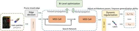
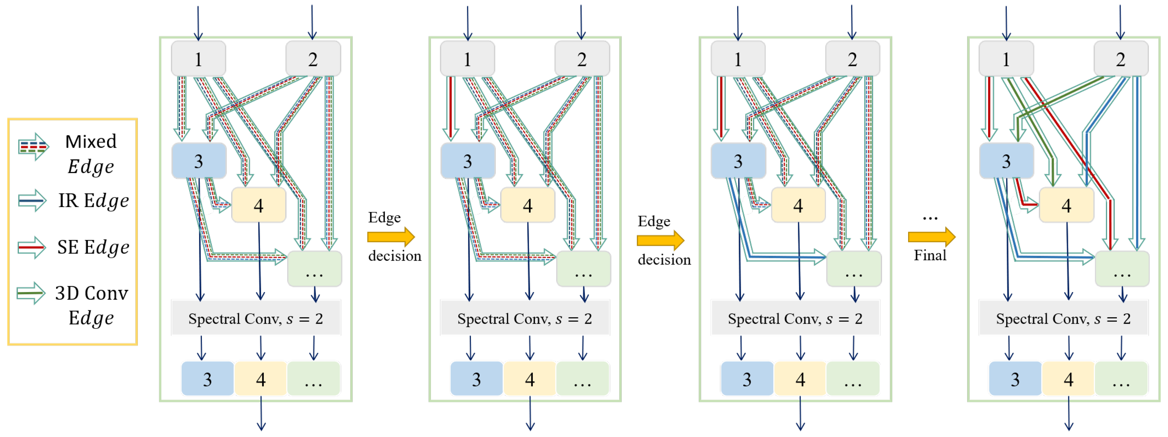
Therefore, inspired by the abovementioned problem and the literature, we construct an efficient attention architecture search (EL-NAS) for HSI classification in this paper. First, because of the efficiency of the GD-based architecture search, we mainly adopt the manner of differentiable neural architecture search as the main automatic DL design strategy to realize the efficient search procedure. Considering the real application for a mobile and embedded device, the lightweight and the attention module and 3D decomposition convolution are simultaneously exploited to construct the searching space, which can efficiently improve the classification accuracy with lower computation and storage costs. Meanwhile, aiming to mitigate the performance collapse caused by the number of skip operations in the searching procedure, the edge decision strategy, and the dynamic regularization is designed by the entropy and distribution of the non-skip operations to preserve the most efficient searching structure. Furthermore, generalization loss is introduced to improve the generalization of the searched model.
We then summarize the main contribution and the innovation of the proposed EL-NAS as follows:
  • EL-NAS successfully introduces the lightweight and attention module and 3D decomposition convolution for automatically realizing the efficient design of DL structure in the hyperspectral image classification area. Therefore, the efficient automatic searching strategy enables us to establish a task-driven automatic design of DL structure for different datasets from different acquisition sensors or scenarios.
  • EL-NAS presents remarkable searching efficiency through edge decision strategy to realize lightweight attention DL structure by imposing (i) the knowledge of successful lightweight 3D decomposition convolution and attention module in the searching space. (ii) The entropy of operation distribution estimated over non-skip operation is implemented to make the edge decision. (iii) Dynamic regularization loss based on the impact of the number of skip connections is adopted for further improving the searching performance. Therefore, the most effective and lightweight operations will be preserved by utilizing the edge decision strategy.
  • Compared with several state-of-the-art methods via comprehensive experiments in accuracy, classification maps, the number of parameters, and the execution cost, EL-NAS presents fewer GPU searching costs and lower parameters and computation costs. The experimental results on three real HSI datasets demonstrate that EL-NAS can search out a more lightweight network structure and realize more robust classification results even under data-independent and sensor-independent scenarios.
The rest of this article is organized as follows. Section 2 reviews the related works in HSI classification. The details of the proposed EL-NAS are described in Section 3. Experiments performance and analysis are designed and discussed in Section 4. Finally, the conclusions are summarized in Section 5 in this article.

2. Related Work

2.1. GD-Based NAS

The search space, search strategy and performance evaluation are main three aspects of GD-based NAS that could be improved. Compared to DARTS, ACA-DARTS [42] removes skip connections from the operation space by introducing an adaptive channel allocation strategy to refill the skip connections in the evaluation stage. PAD-NAS [43] can automatically design the operations for each layer and achieve a trade-off between search space quality and model diversity. In [44], a new search space is introduced based on the backbone of the convolution-enhanced transformer (Conformer), a more expressive architecture than the ASR architecture used in existing NAS-based ASR frameworks. For the re-identification (ReID) task, CDNet [45] is proposed based on a novel search space called the combined depth space (CDS). By using the combined basic building blocks in the CDS, CDNet tends to focus on the combined pattern information normally found in pedestrian images. For hyperspectral image classification task, 3D-ANAS is proposed by a three-dimensional asymmetric decomposition search space, which realized the efficiency improvement of classification [46]. A novel hybrid search space is also proposed in [47], where 3D convolution, 2D spatial convolution and 2D spectral convolution are employed.
Recent research gradually focused on how to avoid the well-known performance collapse caused by an inevitable aggregation of skip connections and mitigate the drawbacks of weight sharing in DARTS. DARTS+ [48] leverages early stopping to avoid the performance collapse in DARTS. PC-DARTS [49] exploits the redundancy of the network space by sampling parts of the supernet for a more efficient search. DARTS- [50] offsets the advantages of a skip connection with an auxiliary skip connection, ensuring more equitable competition for all operations. SGAS [51] partitioned the search process into sub-problems to select and greedily reduce candidate operations. FairNAS [52] suggests strict fairness, where each iteration of the supernet has to train the parameters of each candidate module at each layer, which guarantees that all candidate modules have equal opportunities for optimization throughout the training process. Single-DARTS [53] updates network weights and structural parameters simultaneously in the same batch of data instead of replacing bi-level optimization, which significantly alleviates performance collapse and improves the stability of the architecture search. Zela et al. [54] demonstrated that the various types of regularization can improve the robustness of DARTS to find solutions with better generalization properties. Additionally, β -DARTS [55] proposes a simple-but-efficient Beta-Decay regularization method to regularize the DARTS-based NAS searching process. U-DARTS [56] redesigns the search space by combining the new search space with sampling and parameter-sharing strategies, where the regularization method considers depth and complexity to prevent network deterioration. FP-DARTS [57] constructs two over-parameter sub-networks that formed a two-way parallel hypernetwork by introducing dichotomous gates to control whether the paths were involved in the training of the hypernetwork.

2.2. NAS for HSI

It is usually a trivial and challenging task to realize state-of-the-art (SOTA) neural networks for a specific task with manually designed expert knowledge and effort. PSO-Net [58] is based on Particle Swarm Optimization (PSO) and an evolutionary search method for hyperspectral image data, enabling accelerated convergence. CPSO-Net [59] presents a more efficient continuous evolutionary approach that can speed the generation of architectures as weight-sharing parameters are optimized. Inspired by DARTS, Chen et al. proposed an automatic CNN (Auto-CNN) [60] for HSI classification by introducing a regularization technique named cutout to improve the classification accuracy. Auto-CNN outperformed with fewer parameters than manually designed DL architectures. A hierarchical search space is proposed in 3D-ANAS [46], which searches both topology and network width and introduces a three-dimensional asymmetric decomposition search space with extremely effective classification performance. A2S-NAS [61] proposes a multi-stage architectural search framework to overcome the asymmetric spatial dimension of the spectrum and capture important features. LMSS-NAS [62] proposes a lightweight multiscale NAS with spatial–spectral attention, which is centered on the design of a search space composed of lightweight convolutional operators and the migration of label smoothing losses into the NAS to ameliorate the problem of unbalanced samples.
Based on the efficiency search strategy of DARTS, we additionally adopt the edge decision algorithm to alleviate performance collapse. Simultaneously, considering the lightweight modules and attention module can improve model performance with fewer parameters, we construct EL-NAS to improve the generalization of the searched model, which further makes it more possible for HSI classification method applied on edge devices.

3. Methodology

In this section, we mainly introduce the procedure of our proposed EL-NAS in detail. The overall workflow is illustrated in Figure 1. The modular search space is mainly used to fully exploit the hyperspectral data characteristics and construct an over-parameterized supernet while combining the lightweight module and attention mechanisms for optimal models with high performance and generalization. The regularization-based edge-decision search strategy involves an edge-decision algorithm that significantly accelerates the convergence of the over-parameter supernet and mitigates weight sharing, which can efficiently limit unfair competition in the search process for skip connections. The performance evaluation defines the metrics guidance of the NAS for high-performance and highly generalization models.

3.1. Modular Search Space

In order to realize more efficient and compact search results for hyperspectral image classification task by the NAS method, we propose a modular search space different from DARTS [41]. In the modular search space, modules are regarded as candidate operations rather than simple convolutions, which can exploit the experience of manual architecture design and ensure the stability of search results.
The whole modular search space is illustrated in Figure 2. Each cell is a DAG (Directed Acyclic Graph) consisting of an ordered sequence of N nodes (including two input nodes, N 3 intermediate nodes, and one output node), where each node x ( i ) represents a feature map in network, where i is the order in the DAG. An operation o ( i , j ) that transforms node x ( i ) to node x ( j ) , associated with each directed edge e i , j connects node x ( i ) and node x ( j ) in the DAG. Meanwhile, each intermediate node is connected with all its predecessors. The set of edges E is formulated as
E = { e i , j , 0 i j , 1 < j < N + 2 }
Each edge e i , j contains all candidate operations (alias paths), and DARTS transforms the discrete operation options into a differentiable parameter optimization problem by continuously relaxing the outputs of the different operations through a set of learnable architectural parameters α . For example, the mixed operation o ¯ ( i , j ) taking the feature map x ( i ) as input can be represented as follows:
o ¯ ( i , j ) ( x ( i ) ) = o O e x p ( α o ( i , j ) ) o O e x p ( α o ( i , j ) ) o ( x ( i ) )
where O is the set of candidate operations (i.e., o p 1 , o p 2 , …, z e r o ), o is a specific operation to be applied to x ( i ) , and parameterized by architecture parameters α o ( i , j ) . Each intermediate node x ( j ) is computed by the following formula:
x ( j ) = i < j o ¯ ( i , j ) x ( i )
The input nodes in the DAG are represented by the output of the previous convolution and previous two cells, and the output nodes are represented by concatenating all intermediate nodes.
We learn from experience in manual architecture design and exploit existing modules as the candidate operations of search space, including lightweight module, attention module, and 3D decomposition convolution.
(1)
Lightweight module (i.e., inverted residual block in MobileNetv2 [63], IR) involves pointwise convolution and depthwise separable convolution. The purpose of the inverted residual module is to increase the number of channels by pointwise convolution and then perform depthwise separable convolution in higher dimensions to extract better channel features without significantly increasing the model parameters and computational costs.
(2)
Attention module (i.e., Squeeze-and-Excitation [64], SE) adaptively learns weights for different channels using global pooling and fully connected layers. Hundreds of spectral channels is a significant characteristic of hyperspectral images, where different channels contribute differently to the feature classification task, so the channel attention module is essential as verified in the experimental section.
(3)
3D decomposition convolution. In this paper, 3D convolution is decomposed into two types of decomposition convolution for processing spectral and spatial information, respectively. The principle of 3D decomposition convolution is shown in Figure 3, where a 3D convolution with a kernel size of C × K × K is decomposed into two decomposition convolutions with a kernel size of C × 1 × 1 and 1 × K × K , respectively. This simplifies the complexity of a single candidate operation and allows the search space to yield more possibilities of models, which can significantly reduce the model parameters.
Therefore, our modular search space fully considered the characteristics of hyperspectral data and presented the following improvements: (1) We take patches as input for accelerating the speed of processing, where the down-sampling operation is not essential in this procedure. (2) In order to efficiently extract the discriminative features of SS, we involve 3D decomposition convolution in search space as the candidate operation. (3) By well-designed attention module on the hyperspectral channel, our method can fully exploit spectral discriminant information. (4) The SS information of the HSI dataset is further extracted by using inverse residual module with less parameter.

3.2. Regularization-Based Edge-Decision Search Strategy

How to search the optimal architecture from the discrete search space in a differentiable manner is a key challenge after the construction of modular search space. Therefore, softmax transforms the search for network architectures from selecting discrete candidate operations to optimize the probability of continuous mixed operations.

3.2.1. Bi-Level Optimization

The network weights ω and the architecture parameters α are two parameters need to be optimized. α denotes the weights of different operations/paths on all edges, while ω is the internal parameters in operations. The bi-level optimization problem is presented by using the following formula to jointly optimize α and ω :
min α L v a l ( ω ( α ) , α )
s . t . ω ( α ) = arg min ω L t r a i n ( ω , α )
where L v a l and L t r a i n denote the validation and training losses, respectively. α is the upper-level variable, and ω is the lower-level variable. The optimal α is obtained by the above bi-level optimization formula, and then the final neural architecture is derived by discretization on chosen operations.
The discretization process is to select the operation o ( i , j ) with the highest weight on the directed edge e i , j and discard other operations:
o ( i , j ) = arg max o O α o ( i , j )
The bi-level optimization process mentioned above presents the following problems: (1) In the later period of the search, the number of skip connections in the selected architecture increases sharply, which is liable to resulting in performance degradation. (2) The weight sharing between subnets leads to inaccurate evaluation. Therefore, the edge decision criterion is exploited to alleviate the above-mentioned problem.

3.2.2. Edge Decision Criterion

The design of the selection criterion is crucial to guarantee that the most optimal edge is chosen during edge decision, i.e., maintaining the optimization of the supernet. Two aspects of edges should be considered: edge importance and selection certainty.

Edge Importance

Skip operation on important edges should have a lower weight. Therefore, the edge importance is defined to measure the weight of non-skip operations:
S E I ( i , j ) = o O , o s k i p e x p ( α o ( i , j ) ) o O e x p ( α o ( i , j ) )

Selection Certainty

Denote distribution p o ( i , j ) = e x p ( α o ( i , j ) ) S E I ( i , j ) o O e x p ( α o ( i , j ) ) , o O , o s k i p represents the normalized softmaxed weights of non-skip operation. Selection certainty is defined as the normalized entropy of the operation distribution p o to measure the certainty of distribution:
S S C ( i , j ) = 1 o O , o s k i p p o ( i , j ) l o g ( p o ( i , j ) ) l o g ( | O | 1 )
Then, the edge importance S E I ( i , j ) and the S S C ( i , j ) are normalized to calculate the final score and select the edge with the highest score:
S e ( i , j ) = n o r m a l i z e ( S E I ( i , j ) ) n o r m a l i z e ( S S C ( i , j ) )
where n o r m a l i z e ( · ) denotes the standard M i n M a x scaling regularization. First, an edge e i + , j + is selected greedily according to the above edge decision criterion, i.e., ( i + , j + ) = a r g max ( i , j ) S e ( i , j ) . The corresponding mixture operation o ¯ ( i , j ) is replaced with the optimal operation via o ( i + , j + ) = arg max o O α o ( i + , j + ) . The weights and architectural parameters of the remaining paths within the mixed operation are no longer needed as the architectural parameters, and the network weights are gradually pruned in the optimization iteration for drastically improving the efficiency of search procedure. The remaining over-parameters supernet S (including remaining A and W ) forms a new subproblem, which is also defined based on DAG. Furthermore, the operations on edge are selected iteratively by solving the remaining subproblems. Therefore, the validation accuracy better reflects the final evaluation accuracy as the model discrepancy is minimized in this procedure. Additionally, we provide each intermediate node eventually preserves two input edges. Once a node has two determined input edges, its other input edges will be pruned.

3.2.3. Dynamic Regularization (DR)

Following the determination of the edge decision, the regularization term that considers the quantity of skip connections is chosen to guide the adjustment of the skipped architecture parameters through the regularity factor δ . This approach effectively mitigates the issue of unfair competition among skip connections. More precisely, the dynamic regularity is defined as
α s k i p ( i , j ) ( x ) = δ α s k i p ( i , j ) ( x )
The performance of the architecture is observed to exhibit a distribution closely resembling a Gaussian distribution when influenced by the number of skip connections. Consequently, the symbol δ is introduced to represent this phenomenon:
δ = a e ( n s k i p μ ) 2 2 σ 2
where n s k i p is the number of skip connections in the selected operation. a, μ , and σ are the parameters in the Gaussian distribution. Dynamic regularity ensures that the selection of skip connections is encouraged when the number of skip connections is not enough and discouraged when a large number of skip connections is involved. As illustrated in Figure 4, the suitable number of skip connections will keep the architecture performance at the optimization status so as to avoid performance collapse caused by skip connections. The super-parameter settings of the Gaussian function were estimated by substituting the numerical results into a Gaussian distribution, e.g., a = 0.81 , μ = 1.22 , σ = 2.17 . The whole searching workflow is illustrated in Figure 5, and an independent network without weight sharing is obtained.

3.3. Performance Evaluation

Designing a suitable loss function is a crucial task in the searching procedure for the optimal architecture. The cross-entropy loss L C E measures the difference between the predicted value and the ground truth in the classification task, the loss is defined as
L C E = 1 n k = 1 n ( y k l o g y ^ k + ( 1 y k ) l o g ( 1 y ^ k ) )
where n denotes the number of samples, y k is the ground-truth label of the given sample, and y ^ k is the predicted label.
The generalization ability of the model can be quantified regarding the differences between the training and evaluation metrics. For two models with similar training metrics, the model with better evaluation metrics is more generalizable because it can better predict an unknown dataset. The training dataset is taken in the searching phase to optimize the model weights. The validation dataset is only available for model searching. The generalization loss L g is defined as the difference between the training metrics L C E t r a i n and the validation metrics L C E v a l , which measures the generalization ability of the model and is designed to guide the searching procedure.
L g = | L C E v a l L C E t r a i n |
where | · | is the absolute value. To further improve the robustness and generalization performance of the searched model, we integrated the Beta-Decay regularization [55]. Specifically, the Beta-Decay regularization can impose constraints to keep the values and variances of the activation architecture parameters not too large.
L β = l o g ( k = 1 | O | e α k )
where O is the set of candidate operations and α k is the architectural parameter associated with operation k. We construct the above losses in an automatic way as optimization objectives.
L = L C E + λ 1 L g + λ 2 L β
where λ 1 and λ 2 are the hyperparameters, the learnable parameters can adaptively balance the weights of different losses. The whole procedure of the proposed EL-NAS is summarized in the Algorithm 1.
Algorithm 1 The overall procedure of the proposed EL-NAS.
  • Input: training dataset X T r a i n (training samples X t r a i n and labels Y t r a i n , validation samples X v a l i d and labels Y v a l i d ), test dataset X T e s t , batch size n, decision frequency e
  • Initialization: Modular supernet S (architecture parameters A = { α ( i , j ) } and network weights W = { ω ( i , j ) } ), mixed operation o ¯ ( i , j ) parameterized by α ( i , j ) for each edge e i , j
  • Search Stage:
  •    while exist undetermined edge do
  •       1. input validation samples X v a l i d , and compute the L v a l i d by S ;
  •       2. Update undetermined architecture parameters A by descending A L v a l i d ( W , A ) ;
  •       3. Input training samples X t r a i n , and compute the L t r a i n by S ;
  •       4. Update weights W by descending W L t r a i n ( W , A ) ;
  •       5. Count the number of skip connections in the currently selected operation, compute the regularity factor δ ;
  •       6. adjust the architecture parameters of the skip connections by α s k i p = δ α s k i p ;
  •       7. If the current epoch satisfies decision frequency e, select an edge e i + , j + based on edge decision criterion S e ;
  •       8. Replace o ¯ ( i , j ) with o ( i , j ) = arg max o O α o ( i , j ) ;
  •       9. Delete unchosen weights ω u n c h o s e d ( i + , j + ) from W , remove α u n c h o s e d ( i + , j + ) from A ;
  • Search Output: The final architecture α derived from the selected operation.
  • Evaluation Stage:
  •     Input training set X T r a i n and optimize network weights ω by descending L C E T r a i n ;
  •     for sample x in X T e s t :
  •        Input x into α , and obtain the predicted result;
  • Evaluation Output: The classification results for all test samples X t e s t

4. Experiments

In this section, we mainly introduce five HSI data sets and the evaluation metrics utilized in this paper. The experiments performance, ablation studies, the parameters of the model and the running time are discussed and analyzed. In order to verify the effectiveness of EL-NAS in different scenarios, we also evaluate our method under independent scenarios with the same sensors (IN and SA) and also independent scenarios under different sensor circumstances (IN, UP, HU, SA, and IMDB).

4.1. Hyperspectral Data Sets

Indian Pines (IN) was collected by AVIRIS sensors in northwest India in 1992. This scene has 220 data channels, the spectral range is 0.2 to 2.4 μ m, and the size of each spectral dimension is 145 × 145. The image has a spatial resolution of 20 m/pixel and contains 16 feature categories, in which two-thirds are agriculture and one-third is forests or other natural perennial plants. Figure 6 shows the three-band false color composite of IN images and the corresponding ground truth data, respectively.
The ROSIS-03 sensor recorded the Pavia University (UP) image of the University of Pavia over Pavia in northern Italy. The image captures the urban area around the University of Pavia. The image size is 610 × 340 × 115, the spatial resolution is 1.3 m/pixel, and the spectral coverage is 0.43 to 0.86 μ m. The image contains nine categories. Before the experiment, 12 frequency bands and some samples containing no information were removed. Figure 7 shows the three-band false-color composite of the UP image and the corresponding ground truth data.
The Houston (HU) data set was collected by the Compact Aerial Spectral Imager (CASI) in 2013 on the University of Houston campus and adjacent urban areas. HU has 144 spectral channels, the wavelength range is 0.38 to 1.05 μ m, and the space size of 1905 × 349 is 2.5 m/pixel. It has 15 different ground truth classes with 15,029 marked pixels. Figure 8 shows the three-band false-color composite of the HU image and the corresponding ground truth data.
Salinas (SA) is captured by the 224-band AVIRIS sensor over the Salinas Valley in California and features high spatial resolution (3.7m pixels). The coverage area includes 512 rows by 217 samples. Like Indian Pines, 20 water absorption bands were discarded, leaving 224 bands remaining. The image contains 16 categories. Figure 9 shows the three-band false-color composite of the SA image and the corresponding ground truth data.
The Chikusei (IMDB) data set was collected by Hyperspectral Visible Near-Infrared Cameras (Hyperspec-VNIR-C) in Chikusei, Ibaraki, Japan, on 19 July 2014. It contains 19 classes and has 2517 × 2335 pixels. Its spatial resolution is 2.5 m per pixel. It consists of 128 spectral bands, which range from 363 to 1018 nm. The IMDB dataset was utilized in the sensor-independent scenario to verify the effects of the proposed EL-NAS. Figure 10 shows the three-band false-color composite of the IMDB image and the corresponding ground truth data.

4.2. Experimental Configuration

We take a pixel-centered patch of size 9 × 9 as input data. The classification results are all summarized with the standard deviation of the estimated means by five independent random runs in experiments to avoid possible bias caused by the random sampling. The number of samples in each category in the training set and test set is also shown in Table 1.
All the experiments in this paper are executed under the computer configuration as follows: An Intel Xeon W-2123 CPU at 3.60 GHz with 32-GB RAM and an NVIDIA GeForce GTX 2080 Ti graphical processing unit (GPU) with 27.8-GB RAM. The software environment is the system of 64-bit Windows 10 and DL frameworks of Pytorch 1.6.0.

4.3. Search Space Configuration

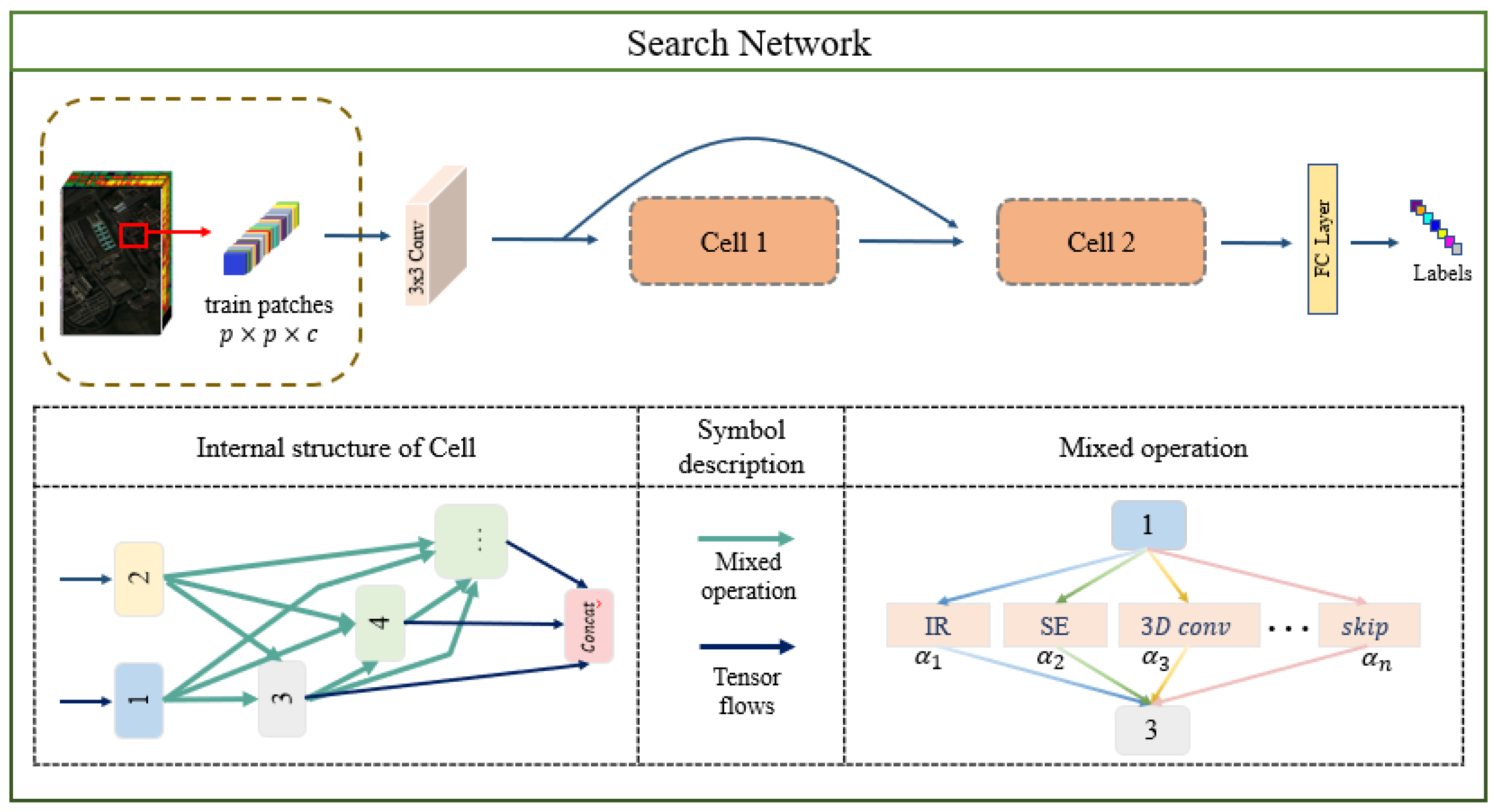
Five types of candidate operations are selected to construct the modular search space (MSS):
  • Lightweight modules ( 3 × 3 and 5 × 5 inverted residual modules, IR).
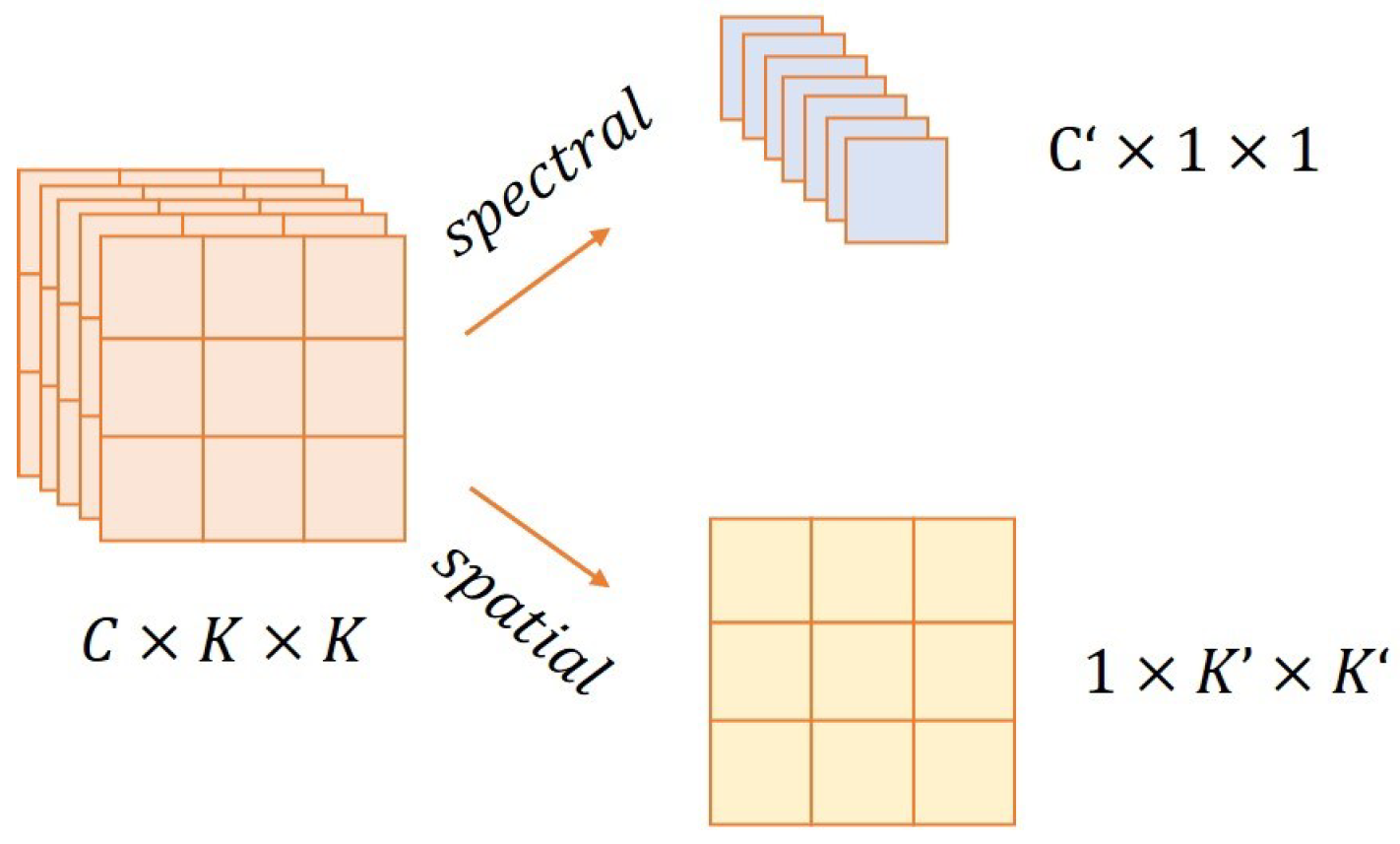
  • Three-dimensional decomposition convolution (3D convolution with kernel size of 1 × 1 × 7 (SPA)and 3 × 3 × 1 (SPE)).
  • Attention modules (SE).
  • Skip connection ( f ( x ) = x ).
  • None ( f ( x ) = 0 ).
During the searching phase, a network is constructed using two normal cells. Within each normal cell, the stride for each convolution is set to 1. Throughout the search process, each cell comprises eight nodes, which include five intermediate nodes and a total of 20 edges.

4.4. Hyperparameter Settings

In the searching phase, we divide the training set into training and validation samples at a ratio of 0.5. Stochastic gradient descent (SGD) is used to optimize the model weight W, the initial learning rate is 0.005, the momentum is 0.9, and the weight decay is 3 × 10 4 . For the architecture parameter A, an Adam optimizer with an initial learning rate of 3 × 10 4 , momentum ( 0.5 , 0.999 ) , and weight decay of 10 3 is used. Edge decisions are made according to the selection criterion, and a complete supernet is not trained during the entire searching phase. After 50 epochs of warm-up, the edge decision is executed every five epochs. In addition, the batch size is increased by 16 after each edge decision, which can further improve the search efficiency.
In the training phase, we perform model training in 1000 epochs with a batch size of 128 and use a random gradient with an initial learning rate of 0.005, a momentum of 0.9, and a weight decay of 3 × 10 4 . The gradient descent optimizer optimizes the model weight W. Other essential hyperparameters include gradient clipping set to 1 and dropout probability set to 0.3.

4.5. Ablation Study

4.5.1. Different Candidate Operations

In this section, we will analyze the effects of different candidate operations and verify the effectiveness of the modular search space, which is shown in Table 2. Based on the comparison between IR and BASE, the results of using the lightweight module are better than the basic convolution. The channel attention SE is ideally suited to datasets with a massive spectrum and significantly boosts performance. The performance of SPE and SPA further improves the performance because of the enhanced ability to extract 3D features of hyperspectral images. We can observe that MSS candidate operations achieved the optimal performance.

4.5.2. Strategy Optimisation Scheme

Three distinct architectural designs were explored within each optimization strategy to assess their impact on the search process. The evaluation results for these architectures are presented in Table 3. The regularization term L β serves to constrain exceedingly large α , thereby allowing for the inclusion of architectural parameters that better represent high-quality architectures. The term L g enhances model performance by approximately 0 . 4 % , corroborating the notion that a more generalized search model is likely to yield an optimally performing architecture. 
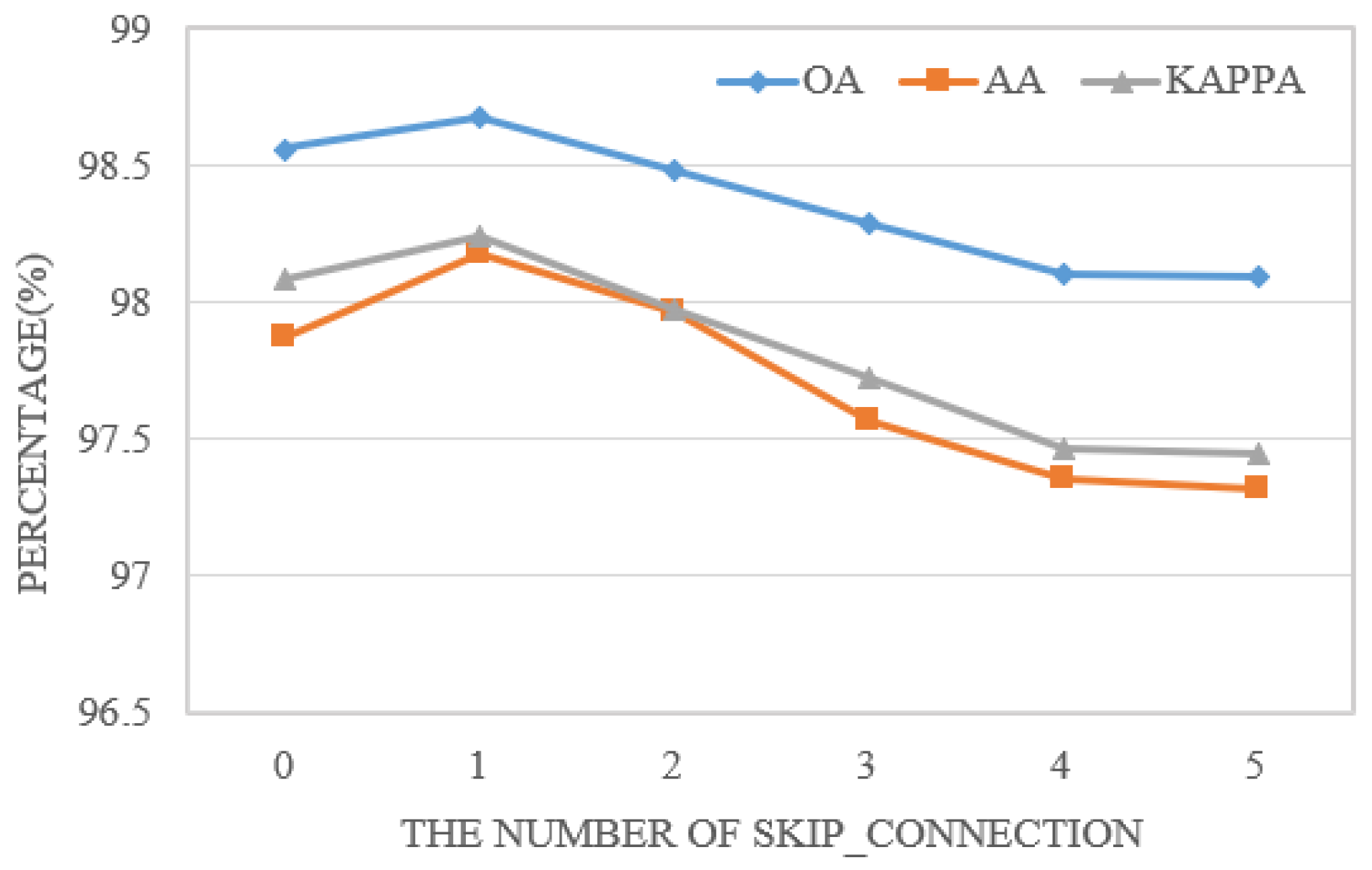
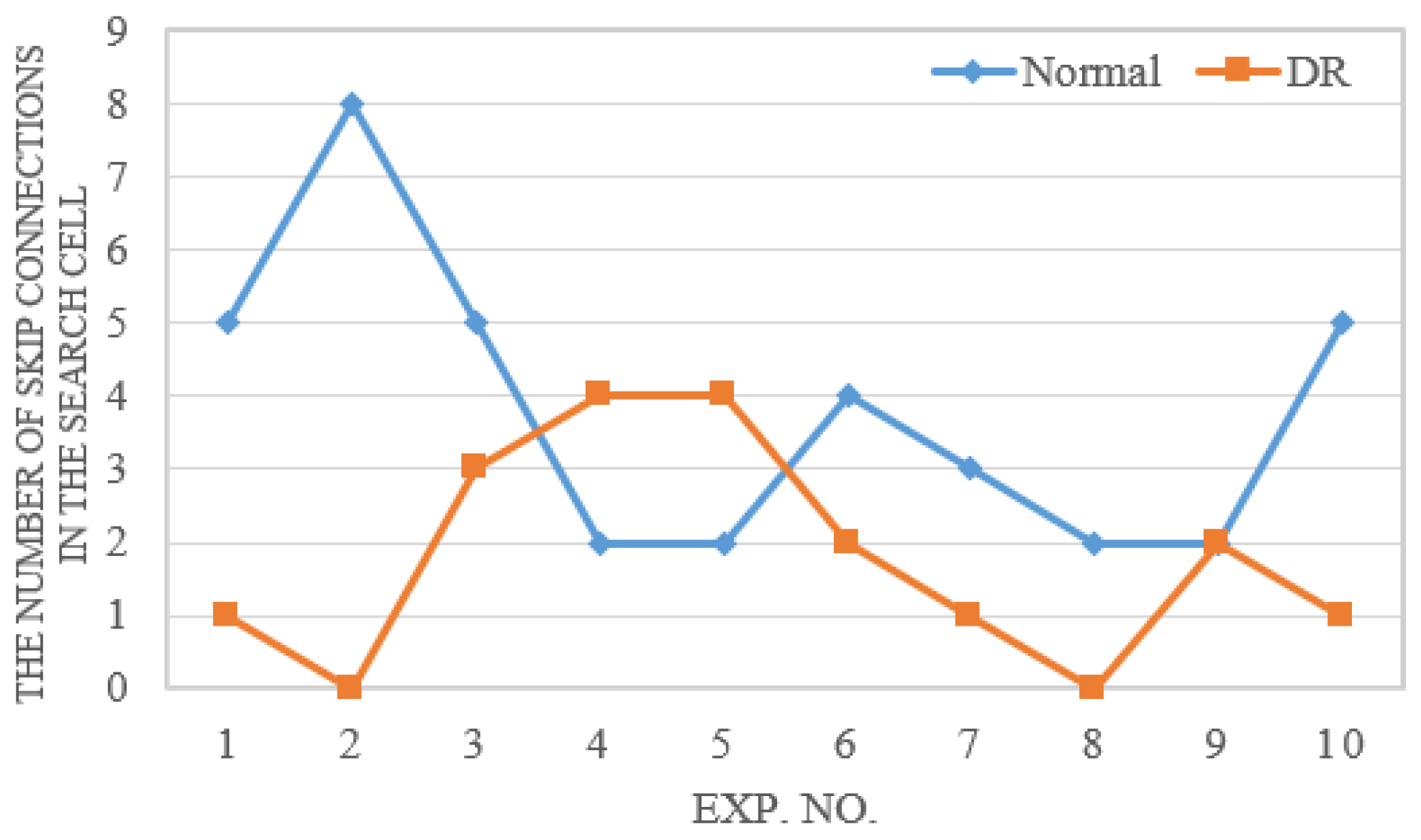
Figure 11 compares the number of skip connections in models with and without Dynamic Regularization (DR) across ten different searches. DR enables the automatic, dynamic adjustment of weights based on the current number of skip connections during each iteration, thereby reducing the frequency of skip operations and leading to more stable search outcomes.

4.6. Architecture Evaluation

In the first set of experiments, we mainly verify the proposed EL-NAS performance under the same scenario (Searching and Test under the same dataset). We randomly select 3 % , 1 % , 3 % of whole labeled samples as the training set, 3 % , 3 % , 3 % of the whole labeled samples as the validation sets, and the remaining 94 % , 96 % , 94 % 
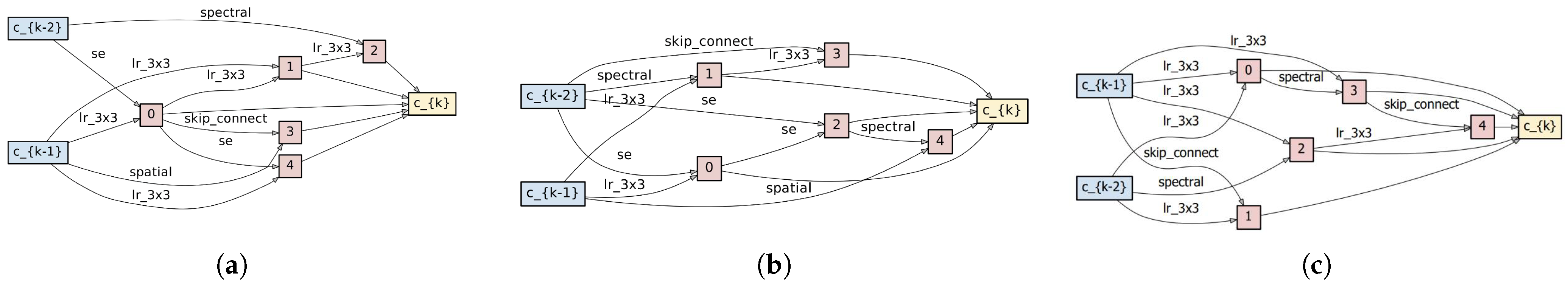
is used as the test set for the three HSI data sets of IN, UP and HU. We first search for the architecture on the training set and reserve an optimal architecture for evaluation. The optimal cell structures obtained from the three data sets are shown in Figure 12. We compare the proposed EL-NAS model with traditional methods SVMCK, six DL methods (2D-CNN, 3D-CNN, DFFN, SSRN, DcCapsGAN, and LMAFN), and one NAS method for HSI classification (Auto-CNN, i.e., 3D-Auto-CNN).
According to the quantitative comparison results shown in Table 4, Table 5 and Table 6, compared with the traditional method SVMCK, DL-based algorithms can achieve better classification results on the three data sets. CNN-based methods can be divided into 2D-CNN and 3D-CNN. Overall, 2D-CNN can extract more discriminative SS features through convolution operation and the nonlinear activation function. Compared with 2D-CNN, 3D-CNN achieves better classification accuracy by fully learning spectral features. Both DFFN and SSRN fuse SS features, and SSRN indicates better results than DFFN. DcCapsGAN integrates GAN and capsule networks to preserve features’ relative location further to improve classification performance. LMAFN adopts lightweight structures, which greatly increases the network depth while reducing the size of the model as well as enhances the nonlinear fitting ability of the model. Additionally, the above traditional algorithms and manually designed DL-based methods are subject to the constraints of subjective human cognition. Auto-CNN achieves satisfactory results in an automated way for neural architecture generation.
Upon a meticulous evaluation of the empirical results, it is evident that the proposed EL-NAS consistently outperforms all comparison algorithms, including Auto-CNN, across the board on all three examined datasets. Specifically focusing on the University of Pavia (UP) dataset, EL-NAS exhibits an exemplary classification accuracy of 98 . 72 % . This result eclipses the performance metrics of other established algorithms as follows: it is 0 . 46 % more accurate than the Spectral–Spatial Residual Network (SSRN) which scores 98 . 26 % , 0 . 72 % higher than DcCapsGAN with 98 . 00 % , 0 . 45 % greater than Lightweight Multiscale Attention Fusion Network (LMAFN) at 98 . 27 % , and notably 1 . 59 % superior to Auto-CNN, which has an accuracy of 97 . 13 % . The superior performance of EL-NAS is due to its innovative integration of a lightweight structure, an attention module, and 3D decomposition convolutions. These elements work synergistically to enhance computational efficiency and focus on key features, contributing to its high classification accuracy. Moreover, EL-NAS leverages automated architecture search, avoiding manual design biases and delivering an optimized, resource-efficient model. This results in better performance metrics across all evaluated datasets, highlighting the algorithm’s efficacy and robustness.
In addition, Table 7 compares the parameter, and network depths of 2D-CNN, 3D-CNN, DFFN, SSRN, DcCapsGAN, LMAFN, and EL-NAS on the three datasets. From Table 7, based on the UP dataset, we can notice that EL-NAS has only 175657 parameters, which is 54 . 2 % less than 443929 parameters of DFFN, 11 . 4 % less than 229261 parameters of SSRN, and 99 . 1 % less than 21468326 parameters of DcCapsGAN. While reducing the model’s size, EL-NAS decreases the network depth to 13 layers and presents the most satisfying accuracies for three different datasets. Table 8 presents the running time of DcCapsGAN, 2D CNN, 3D CNN, DFFN, SSRN, LMAFN, Auto-CNN, and EL-NAS, including searching time, training time, and test time. For the three data sets, our model runs 68.22 s, 62.66 s, and 71.39 s for searching, 87.81 s, 117.81 s, and 147.43 s for training, and 0.88 s, 3.42 s, and 1.28 s for testing, respectively. Note that we use more efficient and complex modules compared to Auto-CNN, so the searched network takes slightly longer to train and test. The execution time of EL-NAS surpasses that of all comparable handcrafted deep-learning algorithms, and its search time also outperforms that of Auto-CNN. This exceptional performance strongly attests to EL-NAS’s high efficiency in both memory utilization and computational overhead. This efficiency is largely attributed to the incorporation of lightweight modules and the expedited search process facilitated by intelligent edge decision-making.
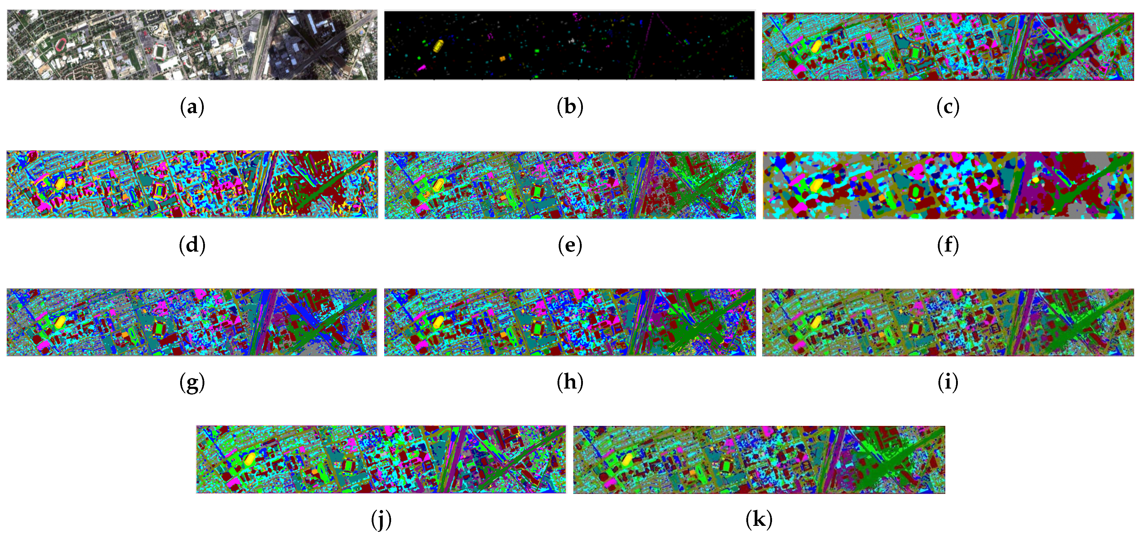
Figure 13, Figure 14 and Figure 15 illustrate the full classification maps obtained from different algorithms on three HSI data sets. Pixel-based approaches SVMCK present more random noise and depict more errors, while SS-based approaches such as 2D-CNN, 3D-CNN, DFFN, SSRN, DcCapsGAN, and LMAFN demonstrate smoother results than pixel-based approaches. In addition, compared with other comparisons, LMAFN exhibits a smoother classification result and higher accuracy because of simultaneously considers spatial and continuous spectral features. Noteworthy, Auto-CNN can obtain precise classification results, which demonstrates the effectiveness of the auto-designed neural network for HSI classification. Nonetheless, when juxtaposed with the aforementioned algorithms, the proposed EL-NAS not only achieves superior accuracy and classification performance, but also does so with a reduced parameter count. This is accomplished through the synergistic integration of lightweight modules and an efficient architecture search algorithm, all underpinned by a highly effective automated architecture search process.

4.7. Cross Domain Experiment

In the second phase of our experiments, we aim to validate the cross-dataset and cross-sensor capabilities of our proposed EL-NAS framework. Specifically, we conduct tests under two distinct scenarios: a dataset-independent scenario, where the neural network architecture is optimized within the same sensor type but across different datasets, and a sensor-independent scenario, where the architecture is optimized across varying sensor types. To facilitate domain adaptation within the classification network, we have engineered dataset-specific classification layers in the latter stages of the network. Additionally, the convolutional layers preceding the shared cells are designed to adapt to diverse datasets.

4.7.1. Cross-Datasets Architecture Search of EL-NAS

In this section, we utilize the IN and SA datasets collected by the AVIRIS sensor for our experiments. EL-NAS is conducted on the IN dataset, and the optimal cell structure identified is then employed to construct the SA classification network. According to Table 9, using the IN dataset for searching yields classification accuracies of 94.70% and 95.99% on the SA dataset with 10 and 20 labeled samples per class, respectively. Conversely, using the SA dataset for searching results in accuracies of 88.60% and 90.39% on the IN dataset with 10 and 20 labeled samples per class, respectively.
The experimental results further substantiate the efficacy of the proposed EL-NAS method in key evaluation metrics. Notably, the use of a substantial auxiliary dataset (labeled as 10% IN or SA) for architecture searching not only matches but often surpasses the performance achieved using the target datasets. These findings offer an efficient methodology for automatic neural network architecture design across different application scenarios under the same acquisition sensor.

4.7.2. Cross-Sensors Architecture Search of EL-NAS

In this part, we adopt five datasets collected by four kinds of HSI acquisition sensors (i.e., IN and SA from AVIRIS, UP from ROSIS, HU from CASI, IMDB from Hyperspec-VNIR-C). We conduct architecture searching on one of the above datasets, and the classification network derived by the searched architecture is applied to other datasets. The experimental results of the search on HU are shown in Table 10. Our findings indicate that when target data volume is limited, the proposed EL-NAS method, utilizing a large auxiliary dataset (labeled as 10% HU), can achieve comparable or superior performance on key evaluation metrics, compared to using target datasets. These results offer an effective optimization strategy for cross-domain learning applications facing data scarcity, demonstrating that EL-NAS can automatically yield a neural network architecture design with satisfactory results even under different datasets collected by different acquisition sensors.

5. Conclusions

In this article, a novel EL-NAS is designed based on the gradient-based NAS manner to realize an efficient automatic way for the application of HSI classification. Meanwhile, the 3D decomposition convolution, lightweight structure, and attention module are considered to construct an efficient, lightweight attention searching space to accelerate the searching procedure and improve the searching results. Further for mitigating performance collapse caused by the number of skip connections in the architecture searching procedure, the edge decision and dynamic regularization are exploited through entropy probability distribution estimation of the non-skip operation and number of skip connections. Meanwhile, with the implementation of edge decisions and decrease in the weight sharing, the consistency in the searching and the evaluation procedure is ensured. In performance evaluation, we also construct a generalization loss to further improve the searching and classification performance. The experiments performed on three different HSI datasets demonstrate that the proposed EL-NAS outperforms other state-of-the-art comparison algorithms in classification accuracy, searching and computationally effectiveness, the number of parameters, and visual comparison performance. In cross scenario experiment, EL-NAS also indicates satisfying performance among different datasets collected by various acquisition sensors. The low searching, parameters, and computational burden of the proposed EL-NAS can further pave a new way for its practical application in HSI classification or edge computing application areas.

Author Contributions

Conceptualization, J.W. and J.H.; methodology, J.W. and J.H.; validation, Y.L., Z.H., S.H. and Y.Y.; investigation, J.W., J.H. and Y.L.; writing—original draft preparation, J.W. and J.H.; writing—review and editing, J.W. and J.H. All authors have read and agreed to the published version of the manuscript.

Funding

This work was supported in part by the National Natural Science Foundation of China under grant numbers 61801353 and 61977052, in part by GHfund B under grant number 202107020822 and 202202022633, and in part by the Project Supported by the China Postdoctoral Science Foundation funded project under grant number 2018M633474, and in part by the, and in part by the China Aerospace Science and Technology Corporation Joint Laboratory for Innovative Onboard Computer and Electronic Technologies under grant number 2023KFKT001-2.

Institutional Review Board Statement

Not applicable.

Informed Consent Statement

Not applicable.

Data Availability Statement

Not applicable.

Conflicts of Interest

The authors declare no conflict of interest. The funders had no role in the design of the study; in the collection, analyses, or interpretation of data; in the writing of the manuscript, or in the decision to publish the results.

References

  1. Lacar, F.M.; Lewis, M.M.; Grierson, I.T. Use of hyperspectral imagery for mapping grape varieties in the Barossa Valley, South Australia. In Proceedings of the Geoscience and Remote Sensing Symposium, Sydney, Australia, 9–13 July 2001. [Google Scholar]
  2. Bioucas-Dias, J.M.; Plaza, A.; Camps-Valls, G.; Scheunders, P.; Nasrabadi, N.; Chanussot, J. Hyperspectral Remote Sensing Data Analysis and Future Challenges. IEEE Geosci. Remote Sens. Mag. 2013, 1, 6–36. [Google Scholar] [CrossRef]
  3. Zhang, F.; Wu, L.; Zhu, D.; Liu, Y. Social sensing from street-level imagery: A case study in learning spatio-temporal urban mobility patterns. ISPRS J. Photogramm. Remote Sens. 2019, 153, 48–58. [Google Scholar] [CrossRef]
  4. Zhang, L.; Zhang, L.; Tao, D.; Huang, X.; Du, B. Hyperspectral remote sensing image subpixel target detection based on supervised metric learning. IEEE Trans. Geosci. Remote Sens. 2013, 52, 4955–4965. [Google Scholar] [CrossRef]
  5. Zhong, Y.; Wang, X.; Xu, Y.; Wang, S.; Jia, T.; Hu, X.; Zhao, J.; Wei, L.; Zhang, L. Mini-UAV-Borne Hyperspectral Remote Sensing: From Observation and Processing to Applications. IEEE Geosci. Remote Sens. Mag. 2018, 6, 46–62. [Google Scholar] [CrossRef]
  6. Chen, Y.; Nasrabadi, N.M.; Tran, T.D. Hyperspectral image classification via kernel sparse representation. IEEE Trans. Geosci. Remote Sens. 2012, 51, 217–231. [Google Scholar] [CrossRef]
  7. Yi, C.; Nasrabadi, N.M.; Tran, T.D. Classification for hyperspectral imagery based on sparse representation. In Proceedings of the Hyperspectral Image and Signal Processing: Evolution in Remote Sensing (WHISPERS), Reykjavik, Iceland, 14–16 June 2010. [Google Scholar]
  8. Melgani, F.; Bruzzone, L. Classification of hyperspectral remote sensing images with support vector machines. IEEE Trans. Geosci. Remote Sens. 2004, 42, 1778–1790. [Google Scholar] [CrossRef]
  9. Peng, J.; Zhou, Y.; Chen, C. Region-Kernel-Based Support Vector Machines for Hyperspectral Image Classification. IEEE Trans. Geosci. Remote Sens. 2015, 53, 4810–4824. [Google Scholar] [CrossRef]
  10. Camps-Valls, G.; Bruzzone, L. Kernel-based methods for hyperspectral image classification. IEEE Trans. Geosci. Remote Sens. 2005, 43, 1351–1362. [Google Scholar] [CrossRef]
  11. Wang, J.; Jiao, L.; Liu, H.; Yang, S. Hyperspectral Image Classification by Spatial–Spectral Derivative-Aided Kernel Joint Sparse Representation. Sel. Top. Appl. Earth Obs. Remote Sens. 2015, 8, 2485–2500. [Google Scholar] [CrossRef]
  12. Wang, J.; Jiao, L.; Shuang, W.; Hou, B.; Fang, L. Adaptive Nonlocal Spatial–Spectral Kernel for Hyperspectral Imagery Classification. IEEE J. Sel. Top. Appl. Earth Obs. Remote Sens. 2016, 9, 1–16. [Google Scholar] [CrossRef]
  13. Saxena, L. Recent advances in deep learning. Comput. Rev. 2016, 57, 563–564. [Google Scholar]
  14. Zhang, H.; Li, Y.; Zhang, Y.; Shen, Q. Spectral-spatial classification of hyperspectral imagery using a dual-channel convolutional neural network. Remote Sens. Lett. 2017, 8, 438–447. [Google Scholar] [CrossRef]
  15. Zhong, Z.; Li, J.; Luo, Z.; Chapman, M. Spectral-Spatial Residual Network for Hyperspectral Image Classification: A 3-D Deep Learning Framework. IEEE Trans. Geosci. Remote Sens. 2017, 56, 847–858. [Google Scholar] [CrossRef]
  16. Slavkovikj, V.; Verstockt, S.; Neve, W.D.; Hoecke, S.V.; Walle, R. Hyperspectral Image Classification with Convolutional Neural Networks. In Proceedings of the the 23rd ACM International Conference, Montreal, QC, Canada, 18–22 October 2021. [Google Scholar]
  17. He, M.; Bo, L.; Chen, H. Multi-scale 3D deep convolutional neural network for hyperspectral image classification. In Proceedings of the 2017 IEEE International Conference on Image Processing (ICIP), Beijing, China, 17–20 September 2017. [Google Scholar]
  18. Mou, L.; Ghamisi, P.; Zhu, X.X. Unsupervised Spectral-Spatial Feature Learning via Deep Residual Conv-Deconv Network for Hyperspectral Image Classification. IEEE Trans. Geosci. Remote Sens. 2018, 56, 391–406. [Google Scholar] [CrossRef]
  19. Song, W.; Li, S.; Fang, L.; Lu, T. Hyperspectral Image Classification With Deep Feature Fusion Network. IEEE Trans. Geosci. Remote Sens. 2018, 56, 3173–3184. [Google Scholar] [CrossRef]
  20. Xi, B.; Li, J.; Diao, Y.; Li, Y.; Li, Z.; Huang, Y.; Chanussot, J. DGSSC: A Deep Generative Spectral-Spatial Classifier for Imbalanced Hyperspectral Imagery. IEEE Trans. Circuits Syst. Video Technol. 2022, 33, 1535–1548. [Google Scholar] [CrossRef]
  21. Zhang, H.; Li, Y.; Jiang, Y.; Wang, P.; Shen, C. Hyperspectral Classification Based on Lightweight 3-D-CNN with Transfer Learning. IEEE Trans. Geosci. Remote Sens. 2019, 57, 5813–5828. [Google Scholar] [CrossRef]
  22. Wang, J.; Guo, S.; Huang, R.; Li, L.; Jiao, L. Dual-Channel Capsule Generation Adversarial Network for Hyperspectral Image Classification. IEEE Trans. Geosci. Remote Sens. 2021, 60, 1–16. [Google Scholar] [CrossRef]
  23. Yang, X.; Cao, W.; Lu, Y.; Zhou, Y. QTN: Quaternion Transformer Network for Hyperspectral Image Classification. IEEE Trans. Circuits Syst. Video Technol. 2023. [Google Scholar] [CrossRef]
  24. Wang, J.; Huang, R.; Guo, S.; Li, L.; Zhu, M.; Yang, S.; Jiao, L. NAS-Guided Lightweight Multiscale Attention Fusion Network for Hyperspectral Image Classification. IEEE Trans. Geosci. Remote Sens. 2021, 59, 8754–8767. [Google Scholar] [CrossRef]
  25. Radosavovic, I.; Kosaraju, R.P.; Girshick, R.; He, K.; Dollar, P. Designing Network Design Spaces. In Proceedings of the IEEE/CVF Conference on Computer Vision and Pattern Recognition (CVPR), New Orleans, LA, USA, 18–24 June 2020. [Google Scholar]
  26. Liu, B.; Yu, X.; Yu, A.; Wan, G. Deep convolutional recurrent neural network with transfer learning for hyperspectral image classification. J. Appl. Remote Sens. 2018, 12, 026028. [Google Scholar] [CrossRef]
  27. He, X.; Chen, Y.; Ghamisi, P. Heterogeneous transfer learning for hyperspectral image classification based on convolutional neural network. IEEE Trans. Geosci. Remote Sens. 2019, 58, 3246–3263. [Google Scholar] [CrossRef]
  28. Liu, X.; Hu, Q.; Cai, Y.; Cai, Z. Extreme learning machine-based ensemble transfer learning for hyperspectral image classification. IEEE J. Sel. Top. Appl. Earth Obs. Remote Sens. 2020, 13, 3892–3902. [Google Scholar] [CrossRef]
  29. Jaderberg, M.; Vedaldi, A.; Zisserman, A. Speeding up Convolutional Neural Networks with Low Rank Expansions. arXiv 2014, arXiv:1405.3866. [Google Scholar]
  30. Hinton, G.; Vinyals, O.; Dean, J. Distilling the Knowledge in a Neural Network. Comput. Sci. 2015, 14, 38–39. [Google Scholar]
  31. Howard, A.; Sandler, M.; Chu, G.; Chen, L.C.; Chen, B.; Tan, M.; Wang, W.; Zhu, Y.; Pang, R.; Vasudevan, V.; et al. Searching for mobilenetv3. In Proceedings of the IEEE/CVF International Conference on Computer Vision, Seoul, Republic of Korea, 27 October–2 November 2019; pp. 1314–1324. [Google Scholar]
  32. Tan, M.; Pang, R.; Le, Q.V. EfficientDet: Scalable and Efficient Object Detection. In Proceedings of the 2020 IEEE/CVF Conference on Computer Vision and Pattern Recognition (CVPR), Seattle, WA, USA, 13–19 June 2020. [Google Scholar]
  33. Wu, H.; Xiao, B.; Codella, N.; Liu, M.; Dai, X.; Yuan, L.; Zhang, L. Cvt: Introducing convolutions to vision transformers. arXiv 2021, arXiv:2103.15808. [Google Scholar]
  34. Leiva-Aravena, E.; Leiva, E.; Zamorano, V.; Rojas, C.; John, M. Neural Architecture Search with Reinforcement Learning. arXiv. 2019, arXiv:1611.01578. [Google Scholar]
  35. Pham, H.; Guan, M.; Zoph, B.; Le, Q.; Dean, J. Efficient neural architecture search via parameters sharing. In Proceedings of the International Conference on Machine Learning, PMLR, Stockholm, Sweden, 10–15 July 2018; pp. 4095–4104. [Google Scholar]
  36. Baker, B.; Gupta, O.; Naik, N.; Raskar, R. Designing neural network architectures using reinforcement learning. arXiv 2016, arXiv:1611.02167. [Google Scholar]
  37. Real, E.; Moore, S.; Selle, A.; Saxena, S.; Suematsu, Y.L.; Tan, J.; Le, Q.V.; Kurakin, A. Large-scale evolution of image classifiers. In Proceedings of the International Conference on Machine Learning, PMLR, Fort Lauderdale, FL, USA, 20–22 April 2017; pp. 2902–2911. [Google Scholar]
  38. Liu, H.; Simonyan, K.; Vinyals, O.; Fernando, C.; Kavukcuoglu, K. Hierarchical representations for efficient architecture search. arXiv 2017, arXiv:1711.00436. [Google Scholar]
  39. Zoph, B.; Vasudevan, V.; Shlens, J.; Le, Q.V. Learning transferable architectures for scalable image recognition. In Proceedings of the IEEE Conference on Computer Vision and Pattern Recognition, Salt Lake City, UT, USA, 18–23 June 2018; pp. 8697–8710. [Google Scholar]
  40. Tan, M.; Chen, B.; Pang, R.; Vasudevan, V.; Sandler, M.; Howard, A.; Le, Q.V. Mnasnet: Platform-aware neural architecture search for mobile. In Proceedings of the IEEE/CVF Conference on Computer Vision and Pattern Recognition, Long Beach, CA, USA, 15–20 June 2019; pp. 2820–2828. [Google Scholar]
  41. Liu, H.; Simonyan, K.; Yang, Y. Darts: Differentiable architecture search. arXiv 2018, arXiv:1806.09055. [Google Scholar]
  42. Li, C.; Ning, J.; Hu, H.; He, K. Enhancing the Robustness, Efficiency, and Diversity of Differentiable Architecture Search. arXiv 2022, arXiv:2204.04681. [Google Scholar]
  43. Xia, X.; Xiao, X.; Wang, X.; Zheng, M. Progressive Automatic Design of Search Space for One-Shot Neural Architecture Search. In Proceedings of the IEEE/CVF Winter Conference on Applications of Computer Vision, Waikoloa, HI, USA, 3–8 January 2022; pp. 2455–2464. [Google Scholar]
  44. Liu, Y.; Li, T.; Zhang, P.; Yan, Y. Improved conformer-based end-to-end speech recognition using neural architecture search. arXiv 2021, arXiv:2104.05390. [Google Scholar]
  45. Li, H.; Wu, G.; Zheng, W.S. Combined depth space based architecture search for person re-identification. In Proceedings of the IEEE/CVF Conference on Computer Vision and Pattern Recognition, Nashville, TN, USA, 20–25 June 2021; pp. 6729–6738. [Google Scholar]
  46. Zhang, H.; Gong, C.; Bai, Y.; Bai, Z.; Li, Y. 3-D-ANAS: 3-D Asymmetric Neural Architecture Search for Fast Hyperspectral Image Classification. IEEE Trans. Geosci. Remote Sens. 2021, 60, 1–19. [Google Scholar] [CrossRef]
  47. Xue, X.; Zhang, H.; Fang, B.; Bai, Z.; Li, Y. Grafting Transformer Module on Automatically Designed ConvNet for Hyperspectral Image Classification. arXiv 2021, arXiv:2110.11084. [Google Scholar]
  48. Liang, H.; Zhang, S.; Sun, J.; He, X.; Huang, W.; Zhuang, K.; Li, Z. Darts+: Improved differentiable architecture search with early stopping. arXiv 2019, arXiv:1909.06035. [Google Scholar]
  49. Xu, Y.; Xie, L.; Zhang, X.; Chen, X.; Qi, G.J.; Tian, Q.; Xiong, H. PC-DARTS: Partial channel connections for memory-efficient architecture search. arXiv 2019, arXiv:1907.05737. [Google Scholar]
  50. Chu, X.; Wang, X.; Zhang, B.; Lu, S.; Wei, X.; Yan, J. DARTS-: Robustly stepping out of performance collapse without indicators. arXiv 2020, arXiv:2009.01027. [Google Scholar]
  51. Li, G.; Qian, G.; Delgadillo, I.C.; Muller, M.; Thabet, A.; Ghanem, B. Sgas: Sequential greedy architecture search. In Proceedings of the IEEE/CVF Conference on Computer Vision and Pattern Recognition, Seattle, WA, USA, 13–19 June 2020; pp. 1620–1630. [Google Scholar]
  52. Chu, X.; Zhang, B.; Xu, R. Fairnas: Rethinking evaluation fairness of weight sharing neural architecture search. In Proceedings of the IEEE/CVF International Conference on Computer Vision, Montreal, QC, Canada, 11–17 October 2021; pp. 12239–12248. [Google Scholar]
  53. Hou, P.; Jin, Y.; Chen, Y. Single-DARTS: Towards Stable Architecture Search. In Proceedings of the IEEE/CVF International Conference on Computer Vision, Nashville, TN, USA, 20–25 June 2021; pp. 373–382. [Google Scholar]
  54. Zela, A.; Elsken, T.; Saikia, T.; Marrakchi, Y.; Brox, T.; Hutter, F. Understanding and Robustifying Differentiable Architecture Search. arXiv 2019, arXiv:1909.09656. [Google Scholar]
  55. Ye, P.; Li, B.; Li, Y.; Chen, T.; Fan, J.; Ouyang, W. beta-DARTS: Beta-Decay Regularization for Differentiable Architecture Search. arXiv 2022, arXiv:2203.01665. [Google Scholar]
  56. Huang, L.; Sun, S.; Zeng, J.; Wang, W.; Pang, W.; Wang, K. U-DARTS: Uniform-space differentiable architecture search. Inf. Sci. 2023, 628, 339–349. [Google Scholar] [CrossRef]
  57. Wang, W.; Zhang, X.; Cui, H.; Yin, H.; Zhang, Y. FP-DARTS: Fast parallel differentiable neural architecture search for image classification. Pattern Recognit. 2023, 136, 109193. [Google Scholar] [CrossRef]
  58. Zhang, C.; Liu, X.; Wang, G.; Cai, Z. Particle Swarm Optimization Based Deep Learning Architecture Search for Hyperspectral Image Classification. In Proceedings of the IGARSS 2020-2020 IEEE International Geoscience and Remote Sensing Symposium, Waikoloa, HI, USA, 26 September–2 October 2020; pp. 509–512. [Google Scholar]
  59. Liu, X.; Zhang, C.; Cai, Z.; Yang, J.; Zhou, Z.; Gong, X. Continuous Particle Swarm Optimization-Based Deep Learning Architecture Search for Hyperspectral Image Classification. Remote Sens. 2021, 13, 1082. [Google Scholar] [CrossRef]
  60. Chen, Y.; Zhu, K.; Zhu, L.; He, X.; Ghamisi, P.; Benediktsson, J.A. Automatic design of convolutional neural network for hyperspectral image classification. IEEE Trans. Geosci. Remote Sens. 2019, 57, 7048–7066. [Google Scholar] [CrossRef]
  61. Zhan, L.; Fan, J.; Ye, P.; Cao, J. A2S-NAS: Asymmetric Spectral-Spatial Neural Architecture Search for Hyperspectral Image Classification. In Proceedings of the ICASSP 2023-2023 IEEE International Conference on Acoustics, Speech and Signal Processing (ICASSP), Rhodes Island, Greece, 4–9 June 2023; pp. 1–5. [Google Scholar]
  62. Cao, C.; Xiang, H.; Song, W.; Yi, H.; Xiao, F.; Gao, X. Lightweight Multiscale Neural Architecture Search With Spectral–Spatial Attention for Hyperspectral Image Classification. IEEE Trans. Geosci. Remote Sens. 2023, 61, 1–15. [Google Scholar] [CrossRef]
  63. Sandler, M.; Howard, A.; Zhu, M.; Zhmoginov, A.; Chen, L.C. MobileNetV2: Inverted Residuals and Linear Bottlenecks. In Proceedings of the IEEE Conference on Computer Vision and Pattern Recognition (CVPR), Salt Lake City, UT, USA, 18–23 June 2018. [Google Scholar]
  64. Hu, J.; Shen, L.; Sun, G. Squeeze-and-excitation networks. In Proceedings of the IEEE Conference on Computer Vision and Pattern Recognition (CVPR), Salt Lake City, UT, USA, 18–23 June 2018; pp. 7132–7141. [Google Scholar]
Figure 1. The search framework of proposed EL-NAS for HSI classification.
Remotesensing 15 04688 g001
Figure 2. The whole modular search space and searching network of the proposed EL-NAS.
Remotesensing 15 04688 g002
Figure 3. The principle of 3D convolution decomposition.
Remotesensing 15 04688 g003
Figure 4. The performance impact of the number of skip connections on Pavia.
Remotesensing 15 04688 g004
Figure 5. The searching workflow works with edge decision with dynamic regularization.
Remotesensing 15 04688 g005
Figure 6. IN. (a) False-color image. (b) Ground-truth map.
Remotesensing 15 04688 g006
Figure 7. UP. (a) False-color image. (b) Ground-truth map.
Remotesensing 15 04688 g007
Figure 8. HU. (a) False-color image. (b) Ground-truth map.
Remotesensing 15 04688 g008
Figure 9. SA. (a) False-color image. (b) Ground-truth map.
Remotesensing 15 04688 g009
Figure 10. IMDB. (a) False-color image. (b) Ground-truth map.
Remotesensing 15 04688 g010
Figure 11. The number of skip connections in the operations selected in ten independent searches.
Remotesensing 15 04688 g011
Figure 12. Best cell architecture on different dataset settings. (a) IN; (b) UP; (c) HU.
Remotesensing 15 04688 g012
Figure 13. Classification maps for IN. (a) False-color image; (b) ground-truth map; (c) SVMCK; (d) 2D-CNN; (e) 3D-CNN; (f) DFFN; (g) SSRN; (h) DcCapsGAN; (i) AUTO-CNN; (j) LAMFN; (k) EL-NAS.
Remotesensing 15 04688 g013
Figure 14. Classification maps for UP. (a) False-color image; (b) ground-truth map; (c) SVMCK; (d) 2D-CNN; (e) 3D-CNN; (f) DFFN; (g) SSRN; (h) DcCapsGAN; (i) AUTO-CNN; (j) LMAFN; (k) EL-NAS.
Remotesensing 15 04688 g014
Figure 15. Classification maps for HU. (a) False-color image; (b) ground-truth map; (c) SVM; (d) SVMCK; (e) 2D-CNN; (f) 3D-CNN; (g) DFFN; (h) SSRN; (i) DcCapsGAN; (j) AUTO-CNN; (k) EL-NAS.
Remotesensing 15 04688 g015
Table 1. Sample setup of IN, UP and HU data sets.
IPUPHU
ClassClass NameTrainTest#ClassClass NameTrainTest#ClassClass NameTrainTest
1Alfalfa251#1Asphalt676963#1Healthy grass381314
2Corn-notill431571#2Meadows18719,582#2Stressed grass381317
3Corn-mintill25913#3Gravel212204#3Synthetic grass21732
4Corn8261#4Trees313218#4Trees381307
5Grass-pasture15532#5Sheets141413#5Soil381305
6Grass-trees22803#6Baresoil515281#6Water10342
7Grass-pasture-mowed131#7Bitumen141397#7Residential391332
8Hay-windrowed15526#8Bricks373867#8Commercial381307
9Oats122#9Shadows10995#9Road381315
10Soybean-nottill301070# #10Highway371289
11Soybean-minttill742701# #11Railway381297
12Soybean-clean18653# #12Parking Lot 1371295
13Wheat7226# #13Parking Lot 215493
14Woods381392# #14Tennis Court13450
15Buildings-Grass-Trees-Drives12425# #15Running Track20693
16Stone-Steel-Towers3103# #
Total3149935#Total43242,344#Total45815,788
Table 2. The performance of different candidate operations.
Condidate OperationsOAAAKAPPA
BASE(dilconv+sepconv) 98.00 ± 0.02 97.59 ± 0.07 97.34 ± 0.03
IR 98.10 ± 0.04 97.57 ± 0.14 97.47 ± 0.05
IR+BASE 98.12 ± 0.16 97.73 ± 0.08 97.50 ± 0.22
IR+SE 98.21 ± 0.12 97.82 ± 0.11 97.61 ± 0.17
IR+pointconv 98.07 ± 0.13 97.72 ± 0.11 97.43 ± 0.18
IR+SPA 98.14 ± 0.04 97 . 83 ± 0 . 07 97.52 ± 0.05
IR+SPE 98.14 ± 0.07 97.82 ± 0.03 97.52 ± 0.10
IR+SPA+SPE 98.16 ± 0.04 97.76 ± 0.16 97.55 ± 0.05
MSS 98 . 27 ± 0 . 09 97.82 ± 0.13 97 . 69 ± 0 . 12
Table 3. The impact of different strategic optimization scheme in three individual searches.
L CE L CE + L β L CE + L β + L g L CE + L β + L g + DR ( δ )
Exp123Mean123Mean123Mean123Mean
OA(%)98.3098.3698.2798.3198.4698.4798.4198.4598.7998.8598.8098.8198.8098.8698.8198.82
AA(%)97.4997.6897.7697.6498.1997.9797.9098.0298.2498.4498.4098.3698.2998.4498.4198.38
KAPPA(%)97.7397.8097.8197.7898.2498.0298.4198.2298.3998.4698.4098.4298.3998.4798.4198.42
Table 4. Classification results of different methods for labeled pixels of the IN data set.
ClassSVMCK2D-CNN3D-CNNDFFNSSRNDcCapsGANAuto-CNNLMAFNEL-NAS
1 79 . 23 ± 6 . 82 78 . 79 ± 1 . 31 30 . 37 ± 2 . 57 90 . 00 ± 8 . 70 76 . 26 ± 20 . 00 11 . 19 ± 0 . 15 68 . 94 ± 2 . 14 83 . 18 ± 15 . 85 68 . 18 ± 6 . 69
2 83 . 60 ± 2 . 97 72 . 68 ± 1 . 45 89 . 58 ± 1 . 15 88 . 35 ± 3 . 54 91 . 98 ± 5 . 03 90 . 49 ± 0 . 25 88 . 95 ± 2 . 40 91 . 95 ± 3 . 40 90 . 57 ± 0 . 36
3 83 . 94 ± 5 . 53 77 . 31 ± 0 . 72 64 . 68 ± 1 . 71 87 . 17 ± 5 . 36 93 . 07 ± 4 . 21 96 . 48 ± 0 . 19 81 . 99 ± 0 . 83 90 . 52 ± 3 . 77 95 . 57 ± 0 . 76
4 79 . 65 ± 5 . 65 77 . 44 ± 2 . 41 53 . 19 ± 1 . 09 92 . 40 ± 4 . 30 77 . 47 ± 13 . 02 72 . 13 ± 0 . 83 79 . 91 ± 2 . 34 93 . 01 ± 5 . 07 87 . 05 ± 3 . 03
5 92 . 70 ± 2 . 95 81 . 41 ± 1 . 07 75 . 34 ± 0 . 12 87 . 99 ± 6 . 43 99 . 75 ± 0 . 35 94 . 67 ± 0 . 01 93 . 38 ± 0 . 63 90 . 60 ± 4 . 37 92 . 09 ± 1 . 51
6 92 . 73 ± 4 . 14 85 . 12 ± 1 . 34 98 . 02 ± 0 . 24 91 . 45 ± 6 . 79 98 . 39 ± 1 . 47 99 . 15 ± 0 . 14 99 . 44 ± 0 . 12 98 . 32 ± 1 . 58 96 . 56 ± 1 . 16
7 95 . 20 ± 1 . 60 4 . 94 ± 2 . 14 44 . 44 ± 0 . 29 77 . 41 ± 23 . 68 86 . 32 ± 9 . 86 32 . 10 ± 2 . 14 60 . 49 ± 14 . 29 90 . 00 ± 16 . 81 96 . 30 ± 3 . 02
8 97 . 59 ± 1 . 66 99 . 78 ± 0 . 08 100 . 00 ± 0 . 00 99 . 00 ± 1 . 54 97 . 41 ± 3 . 66 99 . 93 ± 0 . 12 100 . 00 ± 0 . 00 99 . 09 ± 0 . 96 100 . 00 ± 0 . 00
9 54 . 74 ± 21 . 98 68 . 42 ± 13 . 93 22 . 81 ± 6 . 08 81 . 58 ± 20 . 14 93 . 94 ± 8 . 57 47 . 37 ± 5 . 26 78 . 95 ± 15 . 49 67 . 37 ± 24 . 21 89 . 47 ± 11 . 37
10 84 . 80 ± 4 . 55 79 . 26 ± 4 . 29 71 . 51 ± 0 . 58 88 . 41 ± 5 . 20 89 . 31 ± 11 . 89 91 . 16 ± 0 . 13 83 . 72 ± 1 . 97 92 . 31 ± 4 . 36 93 . 74 ± 0 . 43
11 89 . 39 ± 2 . 14 91 . 01 ± 1 . 24 90 . 54 ± 0 . 42 94 . 72 ± 1 . 06 91 . 27 ± 5 . 54 96 . 82 ± 0 . 06 90 . 02 ± 1 . 61 95 . 30 ± 1 . 55 96 . 72 ± 0 . 72
12 75 . 36 ± 8 . 85 88 . 99 ± 2 . 73 89 . 68 ± 1 . 23 90 . 52 ± 3 . 19 71 . 68 ± 11 . 96 78 . 03 ± 0 . 10 80 . 58 ± 1 . 97 93 . 11 ± 3 . 93 96 . 93 ± 0 . 57
13 99 . 02 ± 0 . 62 96 . 30 ± 0 . 58 99 . 50 ± 0 . 47 90 . 51 ± 8 . 64 96 . 67 ± 2 . 89 99 . 66 ± 0 . 58 99 . 33 ± 0 . 24 98 . 84 ± 0 . 96 99 . 66 ± 0 . 24
14 95 . 86 ± 1 . 62 89 . 95 ± 0 . 53 95 . 65 ± 0 . 05 96 . 81 ± 1 . 88 94 . 93 ± 3 . 12 99 . 13 ± 0 . 12 98 . 91 ± 0 . 20 97 . 74 ± 2 . 16 99 . 59 ± 0 . 20
15 82 . 77 ± 6 . 47 88 . 32 ± 3 . 21 75 . 40 ± 0 . 80 90 . 27 ± 6 . 77 86 . 12 ± 8 . 92 83 . 87 ± 0 . 31 81 . 64 ± 1 . 97 94 . 39 ± 6 . 87 85 . 29 ± 0 . 87
16 95 . 22 ± 4 . 79 75 . 56 ± 4 . 84 72 . 22 ± 0 . 52 58 . 89 ± 8 . 37 93 . 33 ± 5 . 18 98 . 52 ± 0 . 64 88 . 15 ± 14 . 41 95 . 22 ± 6 . 07 88 . 89 ± 1 . 01
OA(%) 88 . 17 ± 1 . 30 84 . 74 ± 0 . 30 85 . 40 ± 0 . 17 91 . 57 ± 1 . 35 89 . 98 ± 0 . 50 93 . 14 ± 0 . 02 89 . 90 ± 0 . 80 94 . 37 ± 0 . 71 94 . 96 ± 0 . 25
AA(%) 86 . 36 ± 2 . 17 78 . 46 ± 1 . 31 73 . 31 ± 0 . 48 87 . 84 ± 3 . 33 89 . 87 ± 1 . 18 80 . 67 ± 0 . 35 89 . 55 ± 1 . 40 91 . 94 ± 3 . 15 93 . 39 ± 0 . 68
KAPPA(%) 86 . 52 ± 1 . 48 82 . 55 ± 0 . 38 83 . 25 ± 0 . 20 90 . 38 ± 1 . 56 88 . 58 ± 0 . 51 92 . 16 ± 0 . 02 88 . 37 ± 0 . 91 93 . 58 ± 0 . 82 94 . 20 ± 0 . 29
PARAM-186,0969068374,880376,89233,521,328176,299148,651274,613
Table 5. Classification results of different methods for labeled pixels of the UP data set.
ClassSVMCK2D-CNN3D-CNNDFFNSSRNDcCapsGANAuto-CNNLMAFNEL-NAS
1 92 . 82 ± 2 . 17 91 . 04 ± 2 . 77 96 . 81 ± 2 . 18 98 . 21 ± 1 . 29 99 . 04 ± 0 . 22 99 . 22 ± 0 . 07 93 . 88 ± 0 . 84 99 . 14 ± 0 . 72 99 . 67 ± 0 . 06
2 98 . 94 ± 0 . 49 97 . 49 ± 1 . 62 90 . 00 ± 15 . 18 99 . 47 ± 0 . 45 99 . 54 ± 0 . 24 99 . 93 ± 0 . 03 99 . 96 ± 0 . 03 99 . 42 ± 0 . 40 99 . 91 ± 0 . 04
3 86 . 40 ± 1 . 84 70 . 97 ± 8 . 52 86 . 15 ± 4 . 14 92 . 37 ± 5 . 47 98 . 76 ± 1 . 31 82 . 23 ± 0 . 07 86 . 11 ± 0 . 61 91 . 50 ± 4 . 23 91 . 63 ± 1 . 38
4 93 . 60 ± 1 . 24 92 . 32 ± 3 . 46 93 . 40 ± 7 . 07 87 . 71 ± 2 . 56 99 . 95 ± 0 . 04 97 . 92 ± 0 . 03 93 . 67 ± 0 . 69 96 . 11 ± 1 . 35 93 . 86 ± 0 . 76
5 99 . 28 ± 0 . 34 99 . 22 ± 0 . 44 96 . 99 ± 4 . 96 95 . 18 ± 4 . 99 99 . 95 ± 0 . 04 99 . 90 ± 0 . 11 99 . 95 ± 0 . 04 99 . 80 ± 0 . 32 99 . 55 ± 0 . 06
6 93 . 98 ± 1 . 65 79 . 90 ± 7 . 80 89 . 64 ± 1 . 50 99 . 40 ± 0 . 93 98 . 79 ± 1 . 47 95 . 81 ± 0 . 03 98 . 33 ± 0 . 22 98 . 80 ± 1 . 13 99 . 72 ± 0 . 15
7 90 . 62 ± 1 . 97 71 . 70 ± 6 . 69 88 . 18 ± 5 . 28 96 . 47 ± 3 . 16 99 . 79 ± 0 . 16 94 . 74 ± 0 . 12 89 . 08 ± 1 . 71 96 . 89 ± 2 . 58 99 . 70 ± 0 . 00
8 93 . 08 ± 1 . 56 92 . 59 ± 4 . 63 87 . 03 ± 3 . 41 96 . 83 ± 2 . 54 88 . 54 ± 2 . 78 97 . 73 ± 0 . 11 97 . 42 ± 0 . 72 95 . 25 ± 1 . 96 97 . 60 ± 0 . 36
9 87 . 92 ± 5 . 22 92 . 93 ± 2 . 35 99 . 75 ± 0 . 16 72 . 57 ± 5 . 23 97 . 22 ± 1 . 49 99 . 61 ± 0 . 12 99 . 40 ± 0 . 13 99 . 18 ± 0 . 81 96 . 69 ± 0 . 31
OA(%) 95 . 41 ± 0 . 50 91 . 48 ± 2 . 10 94 . 21 ± 0 . 44 97 . 03 ± 0 . 70 98 . 26 ± 0 . 07 97 . 97 ± 0 . 03 97 . 13 ± 0 . 05 98 . 27 ± 0 . 49 98 . 72 ± 0 . 12
AA(%) 92 . 96 ± 0 . 68 87 . 57 ± 1 . 97 91 . 99 ± 0 . 82 93 . 13 ± 1 . 21 97 . 95 ± 0 . 17 96 . 34 ± 0 . 03 96 . 15 ± 0 . 14 97 . 34 ± 0 . 75 98 . 26 ± 0 . 09
KAPPA(%) 93 . 91 ± 0 . 66 88 . 62 ± 2 . 81 92 . 27 ± 0 . 59 96 . 06 ± 0 . 92 97 . 69 ± 0 . 09 97 . 30 ± 0 . 04 96 . 16 ± 0 . 07 97 . 73 ± 0 . 46 98 . 30 ± 0 . 15
PARAM-185,1935253443,929229,26121,468,326156,101140,260175,657
Table 6. Classification results of different methods for labeled pixels of the HU data set.
ClassSVMCK2D-CNN3D-CNNDFFNSSRNDcCapsGANAuto-CNNLMAFNEL-NAS
1 97 . 16 ± 1 . 74 90 . 74 ± 2 . 19 96 . 37 ± 0 . 59 93 . 62 ± 2 . 32 97 . 97 ± 2 . 37 98 . 68 ± 0 . 22 98 . 10 ± 0 . 18 97 . 54 ± 2 . 47 97 . 80 ± 0 . 31
2 95 . 99 ± 3 . 32 87 . 21 ± 3 . 01 96 . 38 ± 1 . 08 92 . 80 ± 3 . 11 95 . 34 ± 4 . 60 98 . 08 ± 0 . 17 98 . 88 ± 0 . 10 98 . 60 ± 1 . 30 99 . 29 ± 0 . 04
3 99 . 62 ± 0 . 48 96 . 38 ± 0 . 60 98 . 67 ± 1 . 31 97 . 91 ± 2 . 32 100 ± 0 . 00 97 . 58 ± 0 . 23 97 . 58 ± 1 . 06 99 . 78 ± 0 . 39 99 . 70 ± 0 . 21
4 92 . 02 ± 4 . 06 93 . 93 ± 0 . 84 96 . 85 ± 3 . 74 85 . 61 ± 3 . 77 99 . 66 ± 0 . 32 94 . 09 ± 0 . 13 99 . 83 ± 0 . 12 98 . 26 ± 1 . 83 99 . 81 ± 0 . 17
5 98 . 32 ± 1 . 43 97 . 88 ± 0 . 69 99 . 72 ± 0 . 19 99 . 57 ± 0 . 98 95 . 46 ± 2 . 30 99 . 81 ± 0 . 17 100 . 00 ± 0 . 00 99 . 65 ± 0 . 62 100 . 00 ± 0 . 00
6 90 . 35 ± 4 . 07 70 . 39 ± 1 . 86 97 . 04 ± 2 . 88 88 . 70 ± 5 . 08 100 ± 0 . 00 85 . 71 ± 0 . 32 90 . 48 ± 4 . 33 93 . 08 ± 5 . 00 94 . 71 ± 2 . 49
7 91 . 29 ± 4 . 07 95 . 09 ± 1 . 82 86 . 37 ± 3 . 48 92 . 70 ± 5 . 25 94 . 68 ± 2 . 33 95 . 77 ± 0 . 21 93 . 38 ± 1 . 03 94 . 85 ± 2 . 77 95 . 66 ± 0 . 50
8 86 . 98 ± 2 . 43 76 . 07 ± 4 . 30 73 . 76 ± 3 . 27 87 . 31 ± 5 . 20 97 . 48 ± 1 . 42 76 . 88 ± 0 . 38 85 . 19 ± 0 . 57 90 . 37 ± 2 . 43 85 . 21 ± 0 . 55
9 88 . 90 ± 6 . 12 86 . 43 ± 2 . 82 79 . 63 ± 0 . 96 87 . 95 ± 3 . 65 94 . 76 ± 0 . 91 90 . 83 ± 0 . 34 81 . 82 ± 1 . 48 89 . 77 ± 2 . 82 84 . 71 ± 0 . 17
10 89 . 53 ± 2 . 77 85 . 53 ± 4 . 76 84 . 52 ± 7 . 45 97 . 38 ± 1 . 67 90 . 60 ± 3 . 71 97 . 81 ± 0 . 17 99 . 19 ± 0 . 17 97 . 12 ± 1 . 60 100 . 00 ± 0 . 00
11 86 . 70 ± 2 . 01 82 . 85 ± 1 . 87 88 . 62 ± 4 . 95 96 . 54 ± 3 . 13 85 . 88 ± 6 . 22 89 . 51 ± 0 . 04 95 . 66 ± 0 . 59 96 . 56 ± 2 . 31 97 . 77 ± 0 . 49
12 88 . 95 ± 2 . 18 86 . 18 ± 3 . 59 86 . 32 ± 2 . 28 92 . 58 ± 2 . 63 90 . 77 ± 7 . 53 97 . 07 ± 0 . 44 96 . 15 ± 0 . 43 97 . 43 ± 1 . 62 97 . 83 ± 0 . 58
13 76 . 56 ± 2 . 37 89 . 96 ± 0 . 67 76 . 41 ± 13 . 92 93 . 37 ± 5 . 23 94 . 50 ± 0 . 78 79 . 47 ± 0 . 32 96 . 77 ± 1 . 71 92 . 56 ± 4 . 09 96 . 92 ± 1 . 40
14 97 . 93 ± 1 . 89 92 . 31 ± 0 . 57 95 . 74 ± 5 . 75 99 . 93 ± 2 . 40 100 ± 0 . 00 99 . 92 ± 0 . 14 99 . 68 ± 0 . 11 98 . 10 ± 2 . 45 99 . 68 ± 0 . 30
15 99 . 88 ± 0 . 17 83 . 94 ± 3 . 06 98 . 91 ± 1 . 09 97 . 39 ± 2 . 93 98 . 33 ± 1 . 37 99 . 84 ± 0 . 16 99 . 90 ± 0 . 15 99 . 92 ± 0 . 23 100 . 00 ± 0 . 00
OA(%) 92 . 02 ± 0 . 81 88 . 19 ± 0 . 27 89 . 76 ± 0 . 65 93 . 20 ± 0 . 58 94 . 59 ± 0 . 32 93 . 84 ± 0 . 14 95 . 26 ± 0 . 18 96 . 24 ± 0 . 66 96 . 28 ± 0 . 12
AA(%) 92 . 01 ± 0 . 82 87 . 66 ± 0 . 37 90 . 37 ± 1 . 09 93 . 56 ± 0 . 60 95 . 70 ± 0 . 17 93 . 40 ± 0 . 13 95 . 67 ± 0 . 08 96 . 24 ± 0 . 73 96 . 65 ± 0 . 29
KAPPA(%) 91 . 37 ± 0 . 87 87 . 22 ± 0 . 30 88 . 93 ± 0 . 71 92 . 65 ± 0 . 62 94 . 16 ± 0 . 35 93 . 33 ± 0 . 15 94 . 84 ± 0 . 20 95 . 94 ± 0 . 72 95 . 95 ± 0 . 13
PARAM-185,9678523375,103290,85127,055,608172,373143,658238,292
Table 7. Parameter, depth of different models for three data sets.
DatasetINUPHU
ModelPatameterDepthPatameterDepthPatameterDepth
2D-CNN186,0963185,1933185,9673
3D-CNN906835253385233
DFFN374,88027443,92933375,10327
SSRN376,89213229,26113290,85113
DcCapsGAN33,521,328/21,468,326/27,055,608/
LMAFN148,65157140,26057143,65857
EL-NAS274,61313175,65713238,29213
Table 8. Running times (s) for three datasets: ’Training’ refers to the total duration required for model training. ’Test’ denotes the complete time taken for testing. ’Searching’ indicates the time needed to complete a search.
INUPHU
SearchingTrainingTestSearchingTrainingTestSearchingTrainingTest
DcCapsGAN-148.0722.83-68.4941.08-125.5923.38
2D-CNN-18.434.96-10.5311.21-16.555.32
3D-CNN-50.543.51-23.534.56-43.293.03
DFFN-337.721.10-376.533.98-350.401.54
SSRN-227.3410.47-290.7727.38-350.6611.55
LMAFN-171.230.82-156.431.73-161.130.83
Auto-CNN82.4386.220.8273.56108.982.8889.41132.001.17
EL-NAS68.2287.810.8862.66117.813.4271.39147.431.28
Table 9. Classification results of cross-datasets architecture search of EL-NAS.
Evaluate DataSA 10SA 20IN 10IN 20
Search DataSA 10IN 10%SA 20IN 10%IN 10SA 10%IN 20SA 10%
OA(%)94.1094.7095.5595.9987.9588.6090.0090.39
AA(%)96.0096.2596.8096.7387.9088.5186.3086.41
KAPPA(%)94.2094.0795.6095.5086.8086.9488.1088.97
Table 10. Classification results of cross-sensors architecture search of EL-NAS.
Evaluate DataIMDB 10IMDB 20IN 10IN 20UP 10UP 20SA 10SA 20
Search DataIMDB 10HU 10%IMDB 20HU 10%IN 10HU 10%IN 20HU 10%UP 10HU 10%UP 20HU 10%SA 10HU 10%SA 20HU 10%
OA(%)97.197.899.099.386.988.790.289.091.591.791.992.194.095.896.796.5
AA(%)95.296.497.397.685.887.687.386.188.887.287.888.597.096.997.298.1
KAPPA(%)96.997.898.999.284.987.189.387.787.989.089.190.293.795.194.495.3
Disclaimer/Publisher’s Note: The statements, opinions and data contained in all publications are solely those of the individual author(s) and contributor(s) and not of MDPI and/or the editor(s). MDPI and/or the editor(s) disclaim responsibility for any injury to people or property resulting from any ideas, methods, instructions or products referred to in the content.

