Abstract
Persistent Scatterer Deformation Pattern Analysis Tool, for short PSDefoPAT, was designed to assign each measuring point of an advanced DInSAR data set a best-fitting time series model based on its displacement time series. In this paper, we will outline the operating principles of the tool. The periodic and trend components of a time series model are separately determined based on hypothesis tests. The periodic component is fitted as a sine function, and for the trend component, linear, quadratic, and piecewise linear regression models are considered. Additionally, the tool assesses the goodness-of-fit for each model in the form of the adjusted coefficient of determination value. The tool works fully automatically and thus facilitates the analysis of large data sets, which are becoming more available to the public due to services such as the European Ground Motion Service. Additionally, we demonstrate the capabilities of PSDefoPAT using four case studies characterized by different deformation mechanisms, various extents of active deformation area, and varying density of measuring points. In all cases, we successfully reveal information on the temporal behavior of the deformation not apparent in the typically presented mean deformation velocity maps.
1. Motivation
Differential Interferometric Synthetic Aperture Radar (DInSAR) has become an essential tool to document and analyze ground surface deformation since the first differential interferogram was published in 1993. It mapped the coseismic displacement field of the Landers earthquake in 1992 in California [1]. Documenting the displacement field of earthquakes is part of the geophysical research field of tectonic geodesy, which employs geodetic methods to study crustal deformation processes. The first surface deformation related to earthquakes was documented in the early 1890s based on geodetic triangulation and leveling measurements collected before and after the Nobi earthquake in Japan (1891). However, conducting surveys to map the displacement field of active faults was quite costly and labor-intensive, and could take years until the end of the 20th century. The observation of far-field ground surface deformation was beyond the capabilities of classical ground-based geodetic techniques. Only the development of Global Navigation Satellite Systems (GNSS), such as the Global Positioning System (GPS) in the 1980s and DInSAR in the early 1990s, facilitated periodically conducting surveys over wide areas independently of weather and daylight conditions. With an increase in available data, they quickly replaced the traditional methods in the field of tectonic geodesy [2].
The strong suits of DInSAR are its higher data acquisition frequency, spatial coverage, and lower costs for studies over wide areas compared with traditional ground-based techniques. Its major limitations are temporal and spatial decorrelation, and atmospheric artifacts that may impair estimating the desired displacement rates [3]. Advanced DInSAR techniques, such as Persistent Scatterer Interferometry (PSI), Small Baseline Subset (SBAS) Interferometry, and SqueeSAR™ (an integrated Persistent and Distributed Scatterers (PS and DS) algorithm) were developed to overcome these limitations [4,5,6]. These techniques are capable of monitoring deformation in the line of sight (LOS) of the sensor with millimeter accuracy, in the case of PSI algorithms and SqueeSAR™ [7,8], and sub-centimeter accuracy, for SBAS algorithms [9].
Launching the Sentinel-1 (S1) satellites in 2014 and 2016 made SAR data more accessible for users from both the public and private sectors, consequently leading to the development of ground motion services (GMS) based on advanced DInSAR techniques. One example is the European Ground Motion Service (EGMS), part of the Copernicus land monitoring service. The service provides deformation maps and displacement rates for all countries participating in the Copernicus initiative. The first product is based on all available S1 images between February 2015 and December 2020. A yearly update of the database is planned [10,11]. The amount of accessible data sparks the question of automatized post-processing strategies to extract the relevant information for land use and urban planning as well as disaster risk assessment. The PSI post-processing algorithm by Berti et al. (2013) [12] automatically distinguishes among PSs with a long-term linear, quadratic, or piecewise linear trend. A seasonal component is not taken into consideration. The algorithm presented by Costantini et al. (2018) [13] does consider a seasonal component but was developed for PSs corresponding to buildings. The algorithm presumes that the area of interest (AOI) is an urban area with a dense PS grid. The PSs are clustered with respect to the location and extent of individual buildings, and the PSs not included in one of the clusters are not further analyzed. Afterward, the displacement time series of each cluster are averaged and subsequently labeled as piecewise linear time series or combined seasonal-and-linear time series.
However, ground surface deformation processes can affect urban and rural areas alike. Excluding PSs not associated with a building could cause missing active deformation areas that could become relevant to settlements or infrastructure in the future. Ground surface deformation processes can also be quite complex, and only estimating the trend or only allowing for a certain combination of components may lead to an incomplete understanding of its nature.
In this study, we present the fundamentals and operating principles of Persistent Scatterer Deformation Pattern Analysis Tool (PSDefoPAT). It is designed to automatically assign each displacement time series of an advanced DInSAR data set a best-fitting time series model. The time series is decomposed into its trend, periodic, and residual components. The components can be viewed separately or as an additively composed model. PSDefoPAT also offers parameters to judge the goodness-of-fit for each estimated model. A first version and first results of PSDefoPAT have been previously presented in Evers et al. (2021) [14] and Evers et al. (2022) [15]. This paper is structured into six sections. The background concerning data sources and pre-processing is provided in Section 2. The operating principle of PSDefoPAT and the relevant fundamentals of time series analysis are outlined in Section 3. Results generated with PSDefoPAT are presented and discussed in Section 4. Section 5 and Section 6 provide an overall discussion of the presented tool and our conclusions.
2. Background
2.1. Persistent and Distributed Scatterers
DInSAR exploits the phase of at least two complex SAR images acquired over the same area using either the same sensor or sensors with identical system characteristics at different times to map ground surface deformation. This technique was first demonstrated for Imperial Valley in California using Seasat images [16]. The differential phase is influenced by temporal and geometric decorrelation and changes in the atmosphere between acquisitions. In the worst case, both effects may leave the interferometric phase unusable for ground surface deformation mapping [17,18]. The basic idea to overcome these limitations is to use a time series of differential interferograms to identify pixels characterized by a low noise level. Only those pixels are then used to derive the desired displacement rates instead of the entire differential interferogram. Algorithms that use this approach are generally referred to as advanced DInSAR techniques. There are two types of reflectors typically associated with such pixels: (a) Persistent Scatterers (PS) and (b) Distributed Scatterers (DS). In the case of a PS pixel, the backscattered signal of its ground resolution cell is dominated by one reflector and stable over time. The algorithm PSInSAR™ by Tele-Rilevamento Europa (TRE) is the first implementation of a PSI algorithm [4,19]. However, over the years, many PSI algorithms have been proposed. Some notable algorithms are Stanford Method for Persistent Scatterer (StaMPS) [20], the PSI algorithm by Gamma Remote Sensing [21], and the adaptation of the LAMBDA algorithm to PSI, which was later included in the Spatio-Temporal Unwrapping Network (STUN) [22,23]. Further information on several different PSI algorithms is provided in Crosetto et al. (2016) [24].
In contrast to PSs, DSs do not stand out due to one single reflector. They are characterized by their similarity to adjacent pixels. Processing them together using spatial averaging allows for an improvement in the signal-to-noise ratio (SNR) and thus the extraction of relevant information on the ground surface deformation. SqueeSAR™ by TRE is the first algorithm to successfully jointly process PSs and DSs [6]. Nowadays, advanced DInSAR techniques based on either or both types of reflectors are well-established remote sensing techniques used to map ground surface deformation with millimeter accuracy [7,8,25].
2.2. Ground Motion Services
The capabilities of advanced DInSAR techniques to monitor geo-hazards, e.g., landslides [26] and aseismic displacement [27], human settlements [28], or critical infrastructure [29,30], have been demonstrated over recent years. The numerous applications and precision of advanced DInSAR techniques has led, in connection with the increase in SAR image availability since the S1 satellites were launched, to a number of different ground motion services (GMS) [10].
At this point, we will only briefly report on the most established national endeavors and will focus on the European Ground Motion Service (EGMS). Displacement measurements of different AOIs provided by the EGMS will be used within the scope of this study to demonstrate the capabilities of PSDefoPAT.
2.2.1. National Endeavors
The most progressed initiatives are the ones led by Italy, Norway, and Germany. Norway was the first country to launch its nationwide GMS, InSAR Norway. The first baseline product covering 2015 to 2018 was launched in November 2018. Regular updates are planned. The main goal of the service is the detection and mapping of landslides. More than 100 new potential landslides were detected only months after the launch of InSAR Norway. SAR images are processed with a PSI approach mainly developed by the Norwegian Research Center (NORCE) [10].
The German BodenBewegungsdienst Deutschland was launched a year after the Norwegian GMS. The initiative is led by the Federal Institute for Geosciences and Natural Resources (BGR). The German Aerospace Center (DLR) was contracted to process the S1 images covering Germany with a wide-area PSI approach. The baseline product covers the time from November 2014 to March 2019 [10].
Italy has several regional GMSs implemented. The services process S1 images with a parallelized SqueeSAR™ approach. Two processing strategies are used: (1) deferred deformation maps and (2) near-real-time deformation monitoring. The first strategy provides the user with a database of ground surface deformation maps as snapshots at certain times. The second approach relies on the continuous processing of S1 images coupled with a data mining algorithm to identify anomalous measuring points (MPs), either PSs or DSs, that accelerate or decelerate [10].
2.2.2. European Ground Motion Service
The EGMS [11] constitutes the first application of ground surface deformation monitoring with DInSAR techniques on a continental scale. The service is an addition to the Copernicus land monitoring service funded by the European Commission. The deformation measurements are based on S1 images collected over European states participating in the Copernicus initiative and the United Kingdom. The data are processed by the OpeRatIonal Ground motion INsar ALliance (ORIGINAL) consortium, which is composed of four companies: e-GEOS, TRE Altamira, NORCE, and GAF. Each company uses its own well-established processing chain based on advanced DInSAR techniques. Both PSs and DSs are considered during processing to reach the maximal MP density in urban and rural areas. The EGMS is a coherent and homogeneous service, despite the different processing chains. Overlapping sections between adjacent processing areas were used to harmonize the end product.
The service delivers four products:
- Basic or L2a.
- Calibrated or L2b.
- Ortho or L3.
- A-EPND.
The Basic product constitutes ground surface deformation measurements in the LOS of the S1 sensors in ascending or descending geometries. Since DInSAR techniques only provide relative measurements in space, it is important to tie the measurements to a geodetic reference system and integrate large-scale motions such as those caused by plate tectonics. For the Calibrated product, this is performed by using the ITRF2014 geodetic reference frame and relating the measurements to a large-scale velocity model derived from maintained Global Navigation Satellite Systems (GNSS), provided as the A-EPND product. The Ortho product stems from a combination of ascending and descending Calibrated products to resolve the ground surface deformation in its vertical and east–west components. In order to facilitate the decomposition of the LOS displacements, the Calibrated ascending and descending products are resampled to a 100 × 100 m grid. Additionally, the A-PEND model is used to factor in the south–north component, which is usually difficult to extract from available DInSAR observations. The Ortho product is also tied to the ITRF2014 geodetic reference system.
The first released version of these products considers S1 images from February 2015 to December 2020. A yearly update of the data set is planned. All products are visualized on the EGMS portal (https://egms.land.copernicus.eu/, accessed on 3rd May 2023) online and are available for download.
3. PSDefoPAT—Time Series Analysis Approach
The Matlab-based tool PSDefoPAT assigns each MP resulting from an advanced DInSAR algorithm a best-fitting time series model based on its associated displacement time series. The model provides information on the evolution of the deformation instead of only a snapshot as the mean velocity does [14,15].
A time series is commonly defined as a sequence of measurements of a specific variable, here the displacement of an MP between SAR image acquisitions, in chronological order but not necessarily equidistantly spaced. Time series analysis aims to determine a mathematical model that describes the evolution of the variable over time. A time series is often split into its trend, seasonal, cyclic, and residual components. The trend component describes the long-term evolution of a variable, while the seasonal and cyclic components describe behavior that repeats regularly. In the literature, the periodic behavior of a variable is referred to as seasonal if it is linked to seasonal effects, such as varying weather conditions over the course of a year. Periodicities linked to other causes are subsumed under the term cyclic [31,32]. Here, we will refer to both components as periodic. The tool determines the trend and periodic components of a given time series separately from one another. The resulting deformation model is the sum of the trend and periodic components, while the residual component represents the part of the time series that the model cannot explain.
The tool can be used either manually or in an automated fashion. The main difference is that if the tool is used manually, the user must provide input during each processing step, and only selected MPs are processed. In contrast, if the tool is used in an automatized fashion, all MPs in the data set are processed, and the user only has to provide input at the beginning of the process. The sequence of the processing steps for the automatized version of PSDefoPAT is presented in Figure 1. In this paper, we will focus on the automatized version of our tool, and an overview of the manual usage of the tool is provided in Evers et al. (2021) [14]. The approach used for the automatized version of the tool is demonstrated using two MPs selected from two advanced DInSAR data sets provided by the EGMS. They were selected so that each processing step could be demonstrated and discussed based on an example. The first one is referred to as MP F and is located at top of the dam body of Parapeiros–Peiros Dam in Greece. It was selected because its time series features a piecewise linear trend. The second MP is called MP G and is located on Fehmarnsund Bridge in Germany. Its time series has a periodic component and a piecewise linear trend.
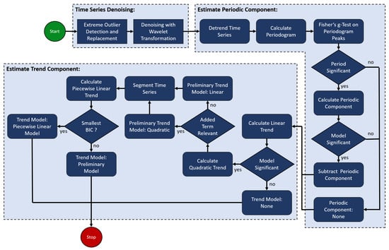
Figure 1.
Workflow of PSDefoPAT.
3.1. Theoretical Background on Time Series Analysis
3.1.1. De-Noising a Time Series
A time series can also be viewed as a combination of noise and a wanted signal. The wanted signal represents any pattern caused by the intrinsic dynamics of the observed process. The time series may additionally be affected by outliers. Outliers are unusual data points in the time series representing possible recording or processing errors. They can have a disruptive effect on time series model selection. PSDefoPAT considers any data point that deviates more than three times the scaled median absolute deviation from the median of the time series to be an extreme outlier. Extreme outliers are replaced using linear interpolation.
Smoothing or de-noising refers to the process of separating the wanted signal in the given time series from noise to reveal patterns previously obscured. An option to smooth the time series is the simple moving average, which replaces the data point recorded at time point T with an average of and J previous data points or an average of and previous and subsequent data points . Similarly, the median could also be used instead of the average. However, a crucial point is to select the right size J of the window, in which the average or median is calculated. The size of the window determines how sensitively the moving average or median reacts to changes in the wanted signal. If the underlying pattern of the wanted signal remains unchanged, a large window is preferred, while a small window is preferable if the underlying pattern changes rapidly over time [31]. Thus, J would need to be selected with a priori knowledge of the time series. An alternative approach to extracting the wanted signal from the provided time series is de-noising using wavelet transformation (WT).
The key factor is that WT can be used to represent any signal. As with any transformation, WT shifts the time series from its original domain into another, possibly making operations such as signal compression or noise reduction easier to conduct [33]. The basic concept of WT is that piecewise regular signals can be described by base wavelet functions, similarly to how Fourier transformation is used to describe a periodic signal as a sum of sine and cosine functions [34].
The basic building block, also referred to as the mother wavelet , of a wavelet basis is a wave-like function that oscillates around zero for a limited time. All other wavelets are generated by dilating or translating the mother wavelet.
The width of the wavelet non-zero part and its position in time are determined by the scaling parameter a and the translation parameter b [33,35].
Noise reduction with WT requires wavelet coefficients derived with discrete wavelet transformation (DWT). The wavelet transform of signal with N data points can be written in vector–matrix form as
where is a vector consisting of N wavelet coefficients and W is an orthogonal matrix containing the wavelet-base vectors. The wavelet base is defined by wavelet filtering coefficients . The number of coefficients varies depending on the wavelet base used. The Daubechies wavelet family, for example, is defined by coefficients. In the case of the second-order Daubechies wavelet, n is 2. The coefficients are used to generate two filters: (1) a scaling filter H, which resembles a low-pass filter, and (2) a wavelet filter G, which is similar to a high-pass filter. The same coefficients define the filters, only in reversed order and with alternating signs. The filter matrices can be written as follows [33]:
and
The filters are used like a recursive pyramid decomposition algorithm, which provides a hierarchical multi-resolution representation of the analyzed signal [36]. At level 1, the scaling and wavelet filters are applied to a signal with N data points, producing detailed coefficients and approximation coefficients . The application of the filters at resolution level m can be written as
and
where denotes the approximation coefficients at a previous resolution level. The original signal can be considered .
At level 2, the filters are applied to the approximation coefficients from level 1, resulting in detailed coefficients and approximation coefficients. The process is repeated until the desired level is reached. The wavelet coefficients consist of both the approximation and detailed coefficients at each resolution level. Thresholding is carried out after applying the filters to the desired resolution level. Since approximation coefficients contain the low-frequency part of the signal, which is usually less affected by noise, thresholding is only applied to detailed coefficients at each level [33,37].
For this purpose, Donoho et al. (1995) introduced the universal threshold [38].
There are two approaches: (1) hard and (2) soft thresholding. Coefficient is dismissed if its absolute value is less than and kept if it surpasses the threshold in case of hard thresholding.
If soft thresholding is applied, the coefficient is also dismissed if its absolute value is smaller than . However, if the absolute value is larger than , it is shifted towards zero by subtracting .
Following thresholding, the remaining coefficients are used to reconstruct the signal [33,37].
PSDefoPAT applies DWT to the entire times series after extreme outliers have been detected and replaced. The wavelet used for DWT is the third Daubechies wavelet. For the noise reduction step, we decided to use soft thresholding because it provides a smooth and continuous time series after signal reconstruction [39].
The effect that noise reduction has on displacement time series can be observed in Figure 2 on the example of MP F and MP G.
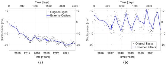
Figure 2.
Original (black) and de-noised displacement time series of (a) MP F and (b) MP G.
3.1.2. Estimation of the Seasonal Component
After reducing the noise level of the time series, the next step to establish a best-fitting time series model is to estimate the periodic component . Displacement time series with a periodic component are often related to the varying water content or temperature of a material. Sine functions are typically used to approximate such phenomena.
where t is the predictor variable, and , , and are the regression coefficients. They represent the amplitude , frequency , and temporal offset with respect to a usual sine function of the modeled time series. PSDefoPAT uses a non-linear least squares approach to fit a sine function to the data points of a given time series. However, this approach requires an initial value for the frequency of the time series.
Fisher’s test [40] is a well-known significance test designed to detect periodicities of unknown frequency in a given time series. The null hypothesis of Fisher’s test assumes that the amplitude of the time series is zero and the signal only consists of Gaussian noise.
The alternative hypothesis assumes that the time series contains a deterministic periodic component with an unknown frequency.
The g-statistic is used as a test statistic for this hypothesis. The statistic is defined by the spectral estimate evaluated at Fourier frequencies [41].
The P-value is formally defined as the probability of obtaining a value from the test statistic at least as extreme or more extreme than the one derived from the data under the assumption that the null hypothesis is true. The value indicates if the data support the null hypothesis sufficiently or not. If the P-value surpasses a predefined level of significance , the null hypothesis is accepted, and if it is smaller, the null hypothesis is rejected [42]. Typical values for are 0.1, 0.05, and 0.01. For PSDefoPAT, the threshold is set to 0.05, meaning that the likelihood of the data to support the null hypothesis is less than 5%. The probability resulting from a g-statistic for a specific peak can be calculated as follows [41]:
Before Fisher’s test is performed on the periodogram of a given time series, the time series is de-trended, i.e., a linear regression model is subtracted from the time series. This step eliminates the presence of the trend component in the periodogram. Afterward, if Fisher’s test identifies a peak in the periodogram with a P-value lower than 0.05, and the associated period is larger than the smallest possible period and smaller than the time interval the time series covers, a sine function is fitted to the de-trended time series. An additional hypothesis test is performed to evaluate if model explains the de-trended time series sufficiently.
The null hypothesis , in this case, assumes that regression model does not sufficiently describe the relationship between the data points of the de-trended time series and predictor variable t.
The test statistic is calculated to determine whether the null hypothesis is rejected or not. The sum of squares due to the regression model , the sum of squares due to the residual error , the number of data points N, the number of predictor variables , and the degree of freedom for the regression model define the -statistic.
The -statistic is used to determine the P-value, which equals the area under the curve of the F-distribution between value and infinity. If the P-value does not exceed the specified level of significance , the null hypothesis is rejected [42]. The threshold is set to 0.05 for PSDefoPAT. In the case of MP E and MP G, the significance test only confirmed a periodic component for MP G. The fitted sine function and the de-trended time series of MP G are presented in Figure 3a.
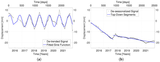
Figure 3.
(a) De-trended and de-noised displacement time series (black) and fitted sine function (blue) for MP G, and (b) de-seasonalized time series (black) and the identified segments (blue) for MP F.
If Fisher’s test identifies a significant period and the subsequent hypothesis test on the fitted sine function results in a P-value lower than 0.05, the predicted values of the periodic component are subtracted from the de-noised time series. The resulting time series is referred to as de-seasonalized.
3.1.3. Estimation of the Trend Component
The last step in determining the best-fitting model for any time series in PSDefoPAT is estimating the trend component. This component describes the long-term evolution of a time series. Three different regression models are considered: (1) linear, (2) quadratic, and (3) piecewise linear trend models.
Linear or quadratic regression models can also be referred to as first- and second-degree polynomial regression models. In general, a k-degree polynomial model can be written as follows:
where denote the regression coefficients; t, the predictor variable; and , the predicted data points. The number of regression coefficients is set to two for a linear regression model. Thus, the equation can be written as follows:
The first- and second-degree polynomial regression models are fitted to the presented data points using ordinary least squares (OLS). The idea is to minimize the squared difference between the measured data points and the data points predicted by the regression model [42].
The procedure is to first estimate a linear regression model, test for its significance, and only estimate the other regression models if a linear relationship between the data points and the predictor variable t could be established. The significance test is performed with an -statistic. The level of significance is set to 0.05, meaning that the likelihood for the data to support the null hypothesis is less than 5%.
A quadratic regression model is fitted to the collected data points only if the linear regression significantly explains the relationship between the data points and the predictor variable. In order to determine if the additional term of the quadratic regression model contributes significantly to the explanation of the collected data points, another hypothesis test is performed. In this case, the null hypothesis assumes that the contribution of the term in question is not significant and can be removed from the regression model.
Student’s t-statistic is used as the test statistic for this hypothesis test instead of the -statistic. The t-statistic is defined by the ratio of the regression coefficient and the associated diagonal element of the variance–covariance matrix .
The contribution of the term in question is considered significant if the associated P-value of the -test statistic is lower than a predefined level of significance . Here, the P-value is defined as the sum of the area underneath the curve of the t-distribution between and infinity, and and negative infinity [31]. The procedure for PSDefoPAT is to accept the quadratic regression model as the preliminary trend model if the P-value is less than 0.05. If not, the linear regression model is accepted as the preliminary trend model.
The last regression model to be estimated is a piecewise linear model, also referred to as piecewise linear representation (PLR). A PLR represents a given time series with N data points as a sequence of K straight lines [43]. The transition point between the two segments is referred to as a change point (CP). A PLR with only one CP can be written as follows [44]:
In order to estimate the PLR of a given time series using a non-linear least squares approach, the number of segments and the location of the associated CPs need to be determined beforehand. Both can be determined using a time series segmentation algorithm. In the literature, a distinction is made between online and offline algorithms. Online algorithms do not have access to the entire time series to produce the best PLR, because they allow data points to be added to the time series in parallel to the execution of the algorithm. On the other hand, for offline algorithms, the time series remains unchanged during the execution of the algorithm, and all data points are taken into consideration to find the best PLR [45].
Keogh et al. (2004) [43] sorts online and offline algorithms in three categories: (1) sliding-window, (2) top-down, and (3) bottom-up algorithms. Algorithms that fall in the category sliding window are considered online algorithms because they do not factor in all the data points of the time series while determining the boundaries of the segments of the PLR. sliding-window algorithms start with the first couple of data points of the time series as the first segment and keep adding data points until the deviation of the approximated segment from the time series exceeds a user-specified threshold. The last added data point is removed and used to form a new segment.
In contrast, top-down and bottom-up algorithms are offline algorithms. Both require the entire time series to determine the boundaries of the segments. A top-down algorithm starts with the assumption that the entire time series is one segment. If the linear approximation of the segments deviates more than the user-specified threshold from the time series, the time series is divided into two segments. Afterward, each segment is recursively tested and further divided until the PLR fulfills the user-specified criterion. bottom-up algorithms, on the other hand, start with the finest possible segmentation of the time series and then merge adjacent segments as long as the resulting PLR does not surpass a user-specified criterion.
Further, there are three different ways to formulate the concrete task of all segmentation algorithms:
- (1)
- Generating the best PLR for the given time series with K segments.
- (2)
- Generating the best PLR of the given time series so that the maximum error of each approximated segment does not exceed a user-specified threshold.
- (3)
- Generating the best PLR of the given time series so that the maximum combined error of all approximated segments does not exceed a user-specified threshold.
We implemented all three types of time series segmentation algorithms with a combination of the first and third formulations of the problem in mind. The first formulation of the task was used so that the number of segments used for the PLR could be limited. Additionally, the choice to use the third instead of the second formulation of the problem in combination with the first one was derived from the goal of PSDefoPAT to find the best-fitting model of the entire time series and not individual segments. The tool uses the mean squared error to evaluate the segmentation. In Figure 3b, the estimated segments of the time series of MP F are marked with blue lines. The procedure for PSDefoPAT is to compare the PLR of the given time series to the previously estimated preliminary trend model. For this reason, the Schwarz–Bayesian Information Criterion (BIC), which is a parameter that evaluates the goodness-of-fit of the regression model in question, is calculated. It is based on the sum of squared residuals or errors, which tends to minimize for more complex models. However, in contrast to criteria such as the adjusted coefficient of determination or the Akaike Information Criterion, it penalizes severely for adding complexity to the regression model and thus avoids over-fitting. The BIC can be calculated as follows [31]:
where N is the number of data points and is the number of predictor variables. The regression model with the lowest value for the BIC is selected as the final trend model.
3.1.4. Evaluation of the Best-Fitting Model and the Residual Component
After estimating the best-fitting model, the sum of the trend and periodic components, it is necessary to evaluate the quality of the selected model. How well the model reproduces the data points of the given time series is referred to as the goodness-of-fit. Two common parameters for the goodness-of-fit are the root mean squared error (RMSE) and the mean absolute error (MAE). The parameters can be calculated as follows:
where N is the number of data points of the given time series and represents the data points predicted by the selected model. Minimizing either parameter yields the best-fitting model in case of normally distributed errors. In the case of a Laplacian-like error, minimizing the MAE provides the best results. Thus, both parameters are reasonable first choices to evaluate the selected model [46].
Another parameter that describes the goodness-of-fit of a time series model is the already mentioned parameter adjusted coefficient of determination . Earlier in this section, it was stated that using leads to over-fitting, which is why it is not used in the context of model selection within PSDefoPAT. However, its typical range, between 0 and 1, caters to an intuitive analysis of the goodness-of-fit of the estimated models in a spatial context. The closer the value is to 1, the better the fit. The parameter is calculated as follows:
where denotes the number of predictor variables in the time series model, N is the number of data points, and SST is the total sum of squares [47]. The estimated best-fitting models of MP E and MP G are presented in Figure 4 with the associated RMSE as upper and lower error margins. Their values are 0.997 and 0.828, respectively.
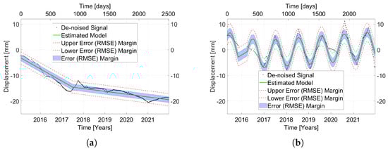
Figure 4.
De-noised time series (black), estimated best-fitting model (green), and associated error margins (blue) for (a) MP F and (b) MP G.
3.2. User Interface
Figure 5 shows the user interface of PSDefoPAT. Both the manual and automated versions of the tool can be operated with the interface. It is structured into three areas. The first area is located in the upper left corner of the interface. The output area is used to display the mean deformation velocity of the MPs in the data set. The second area, in the lower left corner, provides the user with a number of different functions, e.g., selecting an MP to analyze or starting the automated processing of the entire data set. The user has the opportunity to conduct the time series analysis of selected MPs themselves in the area of the interface located on its right side. Input on, e.g., outlier detection or change point detection for a PLR of the time series can be provided. More information on the manual processing of selected MPs can be found in Evers et al. (2021) [14]. In case the automated processing of the entire data set is selected, the user has to provide initial input on the following:
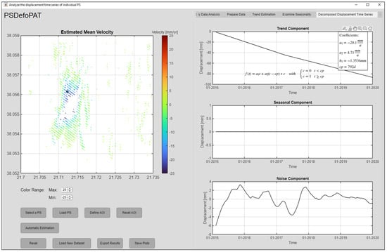
Figure 5.
The user interface of PSDefoPAT showing the components of a fully processed displacement time series.
- (1)
- The maximum number of segments to be used in the PLR of the time series.
- (2)
- The maximum error used to estimate the segments of a PLR.
- (3)
- The type of segmentation algorithm to be used.
Once the parameters are set, they are valid for the entire data set. For the case studies presented in Section 4, we opted for the top-down segmentation algorithm and a maximum number of segments of three. The error threshold for time series segmentation was set to the standard deviation of the de-seasonalized time series.
As for the computational time needed, using the automated process, a small data set, such as the one covering Fehmarnsund Bridge with 9447 MPs, takes roughly a few minutes to be processed. A larger data set, on the other hand, such as the one covering the area of Campi Flegrei with 324,228 MPs, needs a few days to be processed.
4. Demonstration Cases
In this section, we will demonstrate the capabilities of PSDefoPAT with the help of four exemplary case studies:
- (1)
- Campi Flegrei.
- (2)
- Volturno Coastal River Basin.
- (3)
- Parapeiros-Peiros Dam.
- (4)
- Fehmarnsund Bridge.
Each case study was chosen to incorporate a different mechanism driving the observed ground surface deformation. Additionally, attention was paid to selecting areas of different extent and with varying types of land use, which can result in various MP densities.
The region of Campi Flegrei is a densely populated area affected by volcanic activity, alternating phases of inflation and deflation [48,49]. The associated ground surface deformation can be observed over an area of roughly 224.9 km2. The second case study is the Volturno Coastal River Basin. The area is characterized by smaller settlements and agriculture. The surface deformation, subsidence, and possibly a periodic deformation are linked to the consolidation of deposits, urbanization, and groundwater extraction in this area [50]. The affected area extends over roughly 39.2 km2. While the first and second examples cover larger areas, the third and fourth examples deal with smaller areas. The third example is the recently finished Parapeiros–Peiros Dam. The area under observation amounts to roughly 1.1 km2. Here, consolidation of the building and foundation material is expected. However, since the dam body is not homogeneously built, deformation rates may vary greatly [51]. The last example is Fehmarnsund Bridge. The bridge was selected because we expected to observe a periodic deformation signal associated with temperature variations over the course of the year.
The displacement time series for each case study were obtained from the EGMS as their Basic products and cover the time between February 2015 and December 2021. However, the specific time period may vary depending on the orbit of the S1 SAR images used to derive the advanced DInSAR products. All displacement rates are measured in the LOS of the sensor; i.e., a negative displacement represents a movement away from the sensor, and a positive displacement indicates a movement towards the sensor.
4.1. Campi Flegrei
Campi Flegrei is an active volcanic caldera in South Italy, west of Naples. Historical evidence indicates volcanic activity in the area for the past 50,000 years, with the last eruption in 1538. Geodetic measurements, however, to monitor ground surface deformation associated with volcanic activity have only been conducted since 1905. The measurements document a period of deflation until 1950, followed by three episodes of uplift: (1) 1950–1952, (2) 1969–1972, and (3) 1982–1985. GNSS and DInSAR campaigns in recent years revealed that after a period of no significant ground surface deformation, the area has been subject to uplift again since 2011. In the 1950s, the period of unrest was not accompanied by felt seismicity. However, in more recent episodes, the magnitude of seismic events has progressively increased. The ground surface deformation and seismic events were also accompanied by other indicators of volcanic activity, such as degassing. It is unclear if the current unrest is a precursor for an eruption and, if so, when the eruption will take place [48,49].
Figure 6a shows the area as an optical image from 2019 obtained by Google Earth. Figure 6b presents the mean deformation velocities of 324,228 MPs in the area. The mean deformation velocity is given in the LOS, i.e., a negative (dark blue) velocity indicates a movement away from the sensor, and a positive (dark red) is a movement towards the sensor. Here, the limits of the color bar are set to −20 to 20 , some measurements of individual MPs may be larger. Notably, there is a movement towards the sensor depicted at the center of the map with a circular form. The mean velocity at the coastline is at least 20 and lessens inland with a minimum velocity of 0 .
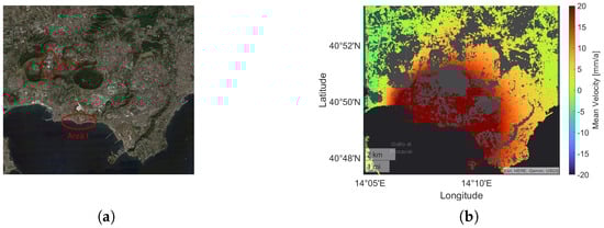
Figure 6.
Area of Campi Flegrei as (a) an optical image obtained from Google Earth and with (b) its mean deformation velocity in the LOS provided by the EGMS.
Since the mean deformation velocity neglects the temporal behavior of the deformation and assumes a linear movement, we further analyzed the data with PSDefoPAT. Our tool assigns each MP in the AOI a best-fitting time series model based on its displacement time series. Selected features of the estimated models are visualized in Figure 7 and Figure 8. Figure 7a indicates if the selected time series models include a periodic component (magenta) or not (cyan). In the case of Campi Flegrei, most MPs in the active deformation area (see Figure 6b) possess time series models that include a periodic component. This varies for MPs located outside of or at the active deformation area’s edge. The amplitude of the periodic component is presented in Figure 7b. The largest amplitudes are observed at the coastline and then decrease inland.
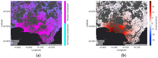
Figure 7.
Visualization of the best-fitting time series model, selected by PSDefoPAT, for each MP at Campi Flegrei showing (a) whether or not the time series model has a periodic component and (b) the amplitude of said periodic component.
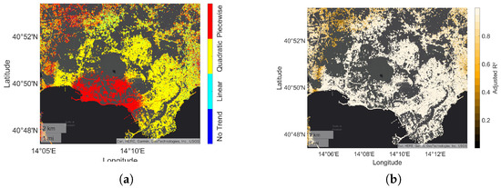
Figure 8.
Visualization of the best-fitting time series model, selected by PSDefoPAT, for each MP at Campi Flegrei depicting (a) the model type of the trend component and (b) the adjusted R value as a measure of the goodness-of-fit.
The type of regression model selected for the trend component is displayed in Figure 8a. A distinction is made between linear (cyan), quadratic (yellow), and piecewise linear (red) regression models. MPs with no trend are colored in dark blue. Figure 8a indicates that the overall deformation pattern of Campi Flegrei can be split into two distinct clusters. The first cluster concentrates on the coastline and exhibits a piecewise linear long-term trend. The second cluster forms a semi-circle around the first cluster and extends more inland. Most MPs located in the area of the second cluster follow a quadratic long-term trend. For MPs outside the active deformation area (see Figure 6b), the choice of the regression model for the trend component varies with no apparent pattern. A look at the adjusted R value depicted in Figure 8b shows that this area is associated with lower adjusted R values, indicating a not sufficiently good fit of the model to the data. Two MPs were chosen to illustrate the compliance of the selected models with the given displacement time series. MP A is located in Area I (marked in Figure 6a) on the coastline, while MP B is located in Area II. The de-noised time series and the selected model of both MPs are presented in Figure 9. MP A follows a piecewise linear trend with a change point after 1038 days. The deformation velocity increases from 68.03 to 92.75 . In addition, the time series of MP A contains a periodic component with an amplitude of 22.14 mm and a period of 1952 days, i.e., roughly five years. However, the proportion of the slopes of the piecewise linear trend to the amplitude of the periodic component begs the question of the geophysical relevance of the periodic component. Even though the results of Fisher’s g-test and the following hypothesis test on the significance of the fitted sine function show that the periodic component is relevant from a time series analysis point of view, Fisher’s g-test resulted in a P-value of 5.42 for the significance of the period, and the likeliness that the periodic component holds no significance to the data points was estimated to be less than 1% P-value = 1.08 ).
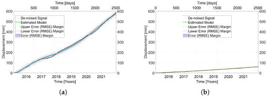
Figure 9.
De-noised displacement time series (black) and estimated best-fitting model (green) with the RMSE as the error margin (blue/red) for (a) MP A in Area I and (b) MP B in Area II.
The time series of MP B has a quadratic long-term trend and no seasonal component. Their displacement time series models are listed in Table 1. They are in good agreement with the measured time series provided by the EGMS. Their R values are 0.996 and 0.998, respectively.

Table 1.
Time series models for the displacement time series of MPs A–H.
The two MPs have in common that their deformation velocity increases during the observation period, which is information not depicted in the mean deformation velocity map (Figure 6b). In addition, PSDefoPAT revealed that the active deformation area (see Figure 6b) can be split into two distinct clusters that follow different trends. The difference in the type of trend indicates that the acceleration of the surface deformation happens more abruptly for the MPs in the first cluster at the coastline compared with those in the second cluster.
4.2. Volturno River Coastal Plain
The Volturno River Coastal Plain is located in the Italian Region Campania north of Naples. It is one of the largest alluvial plains of the Italian peninsula and is subject to subsidence. The deformation is mainly associated with the consolidation of the fluvial and palustrine deposits forming the alluvial plain due to the lithostatic load. Human activities such as water exploitation and urbanization are additional factors that may locally influence the deformation. Both tourist and residential housing experienced a severe increase over the last three decades, affecting both the load due to construction and water-pumping activities. Additionally, a slight uplift can be observed in the east of the area, which relates to tectonic activities [50].
Figure 10a depicts the area as an optical image acquired in 2019 and obtained from Google Earth. Figure 10b shows the mean deformation velocities of 40,279 MPs located in the area in the LOS of the sensor. The range of the color bar is again set to (dark blue) to 20 (dark red). The area at the center of the map in Figure 10b is subject to a movement away from the sensor with a mean velocity of at least .
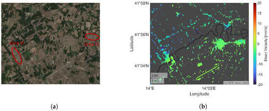
Figure 10.
Area of the Volturno River Coastal Plain as (a) an optical image obtained from Google Earth and with (b) its mean deformation velocity in the LOS provided by the EGMS.
Since the mean deformation velocities do not provide any information on the temporal deformation pattern of the region, we further analyzed the data set with PSDefoPAT. Selected features of the estimated time series displacement models are visualized in Figure 11 and Figure 12. Figure 11a shows if the selected regression models include (magenta) a periodic component or not (cyan). Figure 10b and Figure 11a indicate that most MPs in Area III (marked in Figure 10a) have a periodic and a trend component. MPs in Area IV (marked in Figure 10a) do not seem to have a significant long-term trend component since their mean velocity in Figure 10b depicts them in green, indicating no or only small movements. Figure 11a, however, reveals that MPs located in Area IV have a periodic component, and consideration of Figure 11b shows that the associated amplitude ranges from 1 mm to 5 mm.
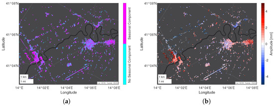
Figure 11.
Visualization of the best-fitting time series model, selected by PSDefoPAT, for each MP at the Volturno River Coastal Plain showing (a) whether or not the time series model has a periodic component and (b) the amplitude of said seasonal component.
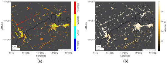
Figure 12.
Visualization of the best-fitting time series model, selected by PSDefoPAT, for each MP at the Volturno River Coastal Plain depicting (a) the model type of the trend component and (b) the adjusted R value as a measure for the goodness-of-fit.
The regression model of the trend component is presented in Figure 12a. Our tool mainly selected, in the case of the Volturno River Coastal Plain, a quadratic trend. Only the north-western corner of the region is characterized by piecewise linear trends. Figure 12b shows that this region is also characterized by lower adjusted R values, indicating a lower goodness-of-fit for the selected time series models.
Two exemplary MPs were selected to highlight specific features revealed by PSDefoPAT. MP C is in Area III, and MP D is in Area IV. Both areas are marked in Figure 10a. Their displacement time series and estimated time series model are shown in Figure 13. Both MPs follow a long-term quadratic trend and have a periodic component. The amplitude of the periodic component of MP C is 7.93 mm, while the amplitude of MP D amounts to 4.75 mm. The goodness-of-fit values for the selected models are 0.982 and 0.979, respectively. Their displacement time series models are listed in Table 1.
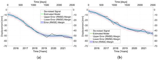
Figure 13.
De-noised displacement time series (black) and estimated best-fitting model (green) with the RMSE as the error margin (blue/red) for (a) MP C in Area III and (b) MP D in Area IV.
This case study illustrates that our tool is capable of revealing active deformation areas, e.g., Area IV, previously not noticeable in the mean deformation velocity map, since it also considers a periodic component for the time series model.
4.3. Parapeiros–Peiros Dam
The third example is a recently finished infrastructure element whose functionality and structural health is crucial for its region. Parapeiros–Peiros Dam, also called Asteri Dam, is located south-west of Patras on the Peloponnese Peninsula in Greece. The dam body is a 75 m high and 760 m long earth-fill embankment dam that impounds the water of the Parapeiros and Peiros Rivers to supply the region with fresh water. The reservoir was designed to store up to 44 m water. The construction of the dam started in mid-2008 and, after some construction freezes, was finished in 2017. The first filling of its reservoir started in September 2019. The dam body was expected to settle after the construction period and during the first filling of the reservoir. The foundation and building material of the dam was expected to consolidate due to its own weight but also due to the increasing load of stored water [51].
Figure 14a depicts the building site, while Figure 14b shows the mean deformation velocities in the LOS for 1251 MPs at the building site during the time from February 2015 to December 2021. The mean deformation velocities on top of the dam body in Figure 14b show a movement away from the sensor at or more. The documented deformation is in good agreement with the expectation that the dam body was to settle after the construction period and during the filling of its reservoir. However, the mean deformation velocities are averaged values and do not provide any information on the temporal progression of the settlement processes. For this reason, we analyzed the data set with PSDefoPAT. Selected features of the resulting best-fitting models and the overall goodness-of-fit are visualized in Figure 15 and Figure 16.
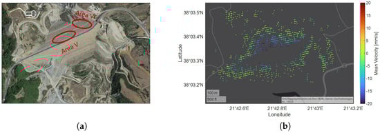
Figure 14.
Building site of Parapeiros-Peiros Dam as (a) an optical image obtained from Google Earth and with (b) its mean deformation velocity in the LOS provided by the EGMS.
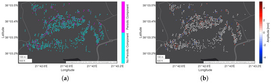
Figure 15.
Visualization of the best-fitting time series model, selected by PSDefoPAT, for each MP at the building site of Parapeiros-Peiros Dam showing (a) whether or not the time series model has a periodic component and (b) the amplitude of said seasonal component.
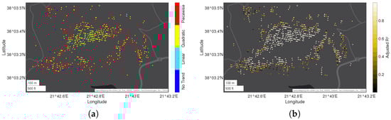
Figure 16.
Visualization of the best-fitting time series model, selected by PSDefoPAT, for each MP at the building site of Parapeiros-Peiros Dam depicting (a) the model type of the trend component and (b) the adjusted R value as a measure for the goodness-of-fit.
Figure 15a shows whether or not the selected model has a periodic component. Cyan denotes that no periodic component is present, while magenta signals the existence of a periodic component. In the case of Parapeiros–Peiros Dam, only a few MPs have a time series model with a periodic component, mostly located at the edges of the dam body. Figure 15b displays the amplitude of the periodic component. Here, most MPs are colored in white, indicating an amplitude of 0 mm.
Figure 16a shows the different regression model types selected for the trend component of the displacement time series of each MP on the dam body. PSDefoPAT picks among a linear model (cyan), a quadratic model (yellow), and piecewise linear model (red). Blue indicates that no trend model was selected. The displacement of the MPs at the center of the dam body close to the crest mostly follows a quadratic model, while a piecewise linear model was selected for MPs at the edges of the dam body. Figure 16b presents the value as an indication of the goodness-of-fit. Notably, the models for the MPs at the center of the downstream shoulder explain the observed displacement rates well. The goodness-of-fit for MPs near the edges of the dam body, however, decreases. For a more detailed view, we selected an MP at the center of the dam body and one closer to the edges to compare their displacement time series. MP E is located in Area V, close to the center of the crest, and MP F is located in Area VI; both are marked in Figure 14a. Their displacement time series and the associated time series model are presented in Figure 17. MP E follows a quadratic trend, while MP F follows a piecewise linear model. Neither one of the models have a periodic component. The goodness-of-fit values are estimated to be 0.997 and 0.903, respectively. Their displacement time series models are listed in Table 1.
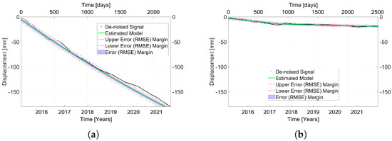
Figure 17.
De-noised displacement time series (black) and estimated best-fitting model (green) with the RMSE as the error margin (blue/red) for (a) MP E in Area V and (b) MP F in Area VI.
Both MPs are also examples of the clusters of MPs they are associated with. Figure 16a reveals that the active deformation area (see Figure 14b) of the dam body can be split into two distinct clusters. The first cluster, at the center of the downstream shoulder, follows a quadratic model, and the second cluster follows a piecewise linear model. The distinction between these clusters indicates that the consolidation of the building and foundation material accelerates differently over time. This might be related to the distribution and processing of the building material, since the dam was not homogeneously built and was subject to construction freezes, which is information that is not apparent in the mean deformation velocity map presented in Figure 14b.
4.4. Fehmarnsund Bridge
The last example is also an infrastructure element, but in contrast to the third example, it has already been in use for several years. Fehmarnsund Bridge, located in North Germany, has been in use since 1963. The bridge connects the German mainland and the German island of Fehmarn over the 1.3 km wide Fehmarnsund. The bridge accommodates both road and rail traffic. It was designed as a high bridge with a 248 m long arched supporting structure [52]. As with many infrastructure elements, we expected the bridge to be sensitive to the ambient temperature and exhibit periodical deformation.
Figure 18a shows the bridge in an optical image obtained from Google Earth, while Figure 18b presents the mean deformation velocity for 9447 MPs located on and close to the bridge. In contrast to the previous examples, the mean velocities range from (dark blue) to 5 (dark red). The coloration of Figure 18b indicates that no significant movements at the bridge could be recorded.
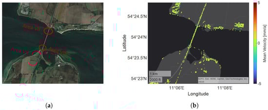
Figure 18.
Building site of Fehmarnsund Bridge as (a) an optical image obtained from Google Earth and with (b) its mean deformation velocity in the LOS provided by the EGMS.
Figure 19 and Figure 20 depict selected features of the time series model assigned to each MP based on their displacement time series utilizing PSDefoPAT. Figure 19 reveals two distinct clusters, Area VII and Area VIII (marked in Figure 18a), on the bridge where most MPs have a seasonal component. Fehmarnsund Bridge is subject to thermal expansion due to environmental influences. However, it is unclear whether the MPs between those two areas are more likely to have a periodic component or not since they do not form a coherent cluster. Taking into account Figure 19b, which presents the amplitude of the periodic component, it is noticeable that the periodic components for MPs of Area VII and those of Area VIII proceed inversely to each other. The reason for this is that the displacement of the MPs is measured in the LOS of the sensor; therefore, one side of the bridge moves towards the sensor, and the other, away from it, leading to inverse amplitudes for the cyclic component. The displacement time series of MP G and MP H from both areas are presented in Figure 21, illustrating the phase shift between the periodic components. The time series models are listed in Table 1.
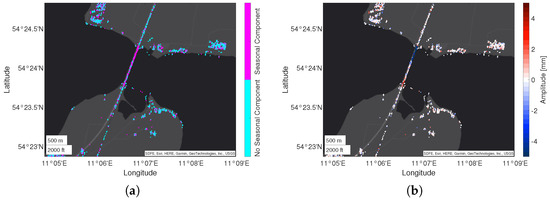
Figure 19.
Visualization of the best-fitting time series model, selected by PSDefoPAT, for each MP at the building site of Fehmarnsund Bridge showing (a) whether or not the time series model has a periodic component and (b) the amplitude of said seasonal component.
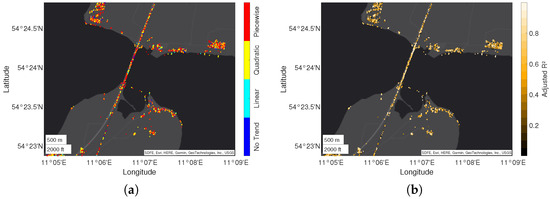
Figure 20.
Visualization of the best-fitting time series model, selected by PSDefoPAT, for each MP at the building site of Fehmarnsund Bridge depicting (a) the model type of the trend component and (b) the adjusted R value as a measure for the goodness-of-fit.
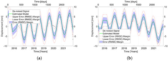
Figure 21.
De-noised displacement time series (black) and estimated best-fitting model (green) with the RMSE as the error margin (blue/red) for (a) MP G in Area VII and (b) MP H in Area VIII.
The regression model for the trend component is presented in Figure 20a. A distinction is made among linear (cyan), quadratic (yellow), and piecewise linear (red) models. MPs with no trend component are marked in dark blue. Most MPs on and close to the bridge have a piecewise linear trend model. However, it is worth mentioning that the slopes of the segments only range between 2 and −2.5 and thus might not be relevant.
In addition, Figure 20b shows the adjusted R value for each regression model as an indication of the goodness-of-fit. Notably, the MPs between Area VII and Area VIII have a lower R value than those associated with Areas VII and VIII. The cause could be a missed periodic component.
Overall, it can be said that the last example illustrates that PSDefoPAT can be used to reveal relevant active deformation areas not apparent in mean deformation velocity maps.
5. Discussion
In the previous section, we demonstrated the capabilities of PSDefoPAT based on four different case studies:
- (1)
- Campi Flegrei.
- (2)
- Volturno Coastal River Basin.
- (3)
- Parapeiros–Peiros Dam.
- (4)
- Fehmarnsund Bridge.
The examples included small- and large-scale deformation patterns, and rural and urban areas. During the selection of the case studies, attention was also paid to the underlying mechanism resulting in the observed ground surface deformation. Campi Flegrei is subject to volcanic activity, alternating phases of inflation and deflation [48,49]. The Volturno Coastal River Basin is affected by both naturally occurring processes, i.e., the consolidation of fluvial and palustrine deposits, and human activity in the form of water exploration and urbanization [50]. The last two examples are infrastructure elements affected by post-building deformation in the form of settlement and thermal expansion due to temperature variation over the course of the year.
In all cases, PSDefoPAT could reveal information on the temporal behavior of the MPs previously not apparent in the presented mean deformation velocity maps. The estimated displacement time series models, their values, and the previously estimated mean deformation velocity are presented in Table 1. The example of MP A and MP B shows that only considering the mean deformation velocity deprives the analyst of the information that the ground surface deformation is accelerating, i.e., the slope of the trend component of the time series model increases, and similarly that the deformation of MP E and MP F is decelerating, i.e., the slope of the trend component of the time series model decreases. Comparing the mean deformation velocity of MP G and MP H with their estimated displacement time series models shows that our tool is also capable of revealing previously neglected active deformation areas by considering a periodic component. The mean deformation velocity of MP G was estimated to be 0.6 , while the displacement time series has a periodic component with an amplitude of −5.35 mm. Similarly, MP H has a periodic component with an amplitude of 3.93 mm, and its mean deformation velocity was estimated to be −0.9 .
Notably, presenting selected features of the estimated time series models in a spatial context showed that PSDefoPAT can be used to divide active deformation areas into multiple clusters of MPs that follow different time series models. This became particularly evident in the example of the region of Campi Flegrei in South Italy and Parapeiros–Peiros Dam in Greece. The active deformation area of Campi Flegrei was decomposed into one area close to the shoreline that follows a piecewise linear trend and a second cluster further inland that follows a quadratic trend. Similarly, PSDefoPAT revealed that the dam body of Parapeiros–Peiros Dam does not deform uniformly. MPs located close to the crest of the downstream shoulder follow a quadratic trend, while MPs closer to the edges of the construction follow a piecewise linear trend. This might be linked to the heterogeneous distribution of building materials and several construction freezes the dam was subject to [51].
Overall, it can be said that PSDefoPAT can be used to reveal information relevant to assessing the temporal behavior of numerous MPs, which would otherwise only be performed for selected MPs and thus not allow for the interpreting of different displacement time series models in a spatial context.
6. Conclusions and Outlook
In this paper, we outlined the operating principle of the Persistent Scatterer Deformation Pattern Analysis Tool, for short PSDefoPAT. The tool was designed to assign each MP of an advanced DInSAR data set a best-fitting time series model based on its displacement time series. It separately estimates a periodic component and a trend component based on hypothesis tests. The periodic component is determined with Fisher’s test on the periodogram of a given time series and fitted as a sine function. For the trend component, the tool selects a model among the linear, quadratic, and piecewise linear regression models. Additionally, the tool assesses the goodness-of-fit for each model in the form of the adjusted coefficient of determination value. PSDefoPAT can be used manually or in a fully automatized fashion. The automatized use of the tool facilitates the analysis of large data sets, which are becoming more available to the public due to services such as the EGMS.
Additionally, we demonstrated the capabilities of PSDefoPAT using four case studies: (1) Campi Flegrei, (2) Volturno Coastal River Basin, (3) Parapeiros–Peiros Dam, and (4) Fehmarnsund Bridge. During the selection of the case studies, special attention was paid to the different underlying mechanisms resulting in the observed ground surface deformation. While Campi Flegrei is subject to a naturally occurring process, i.e., volcanic activity, the Volturno Coastal River Basin is affected by both naturally occurring processes, i.e., the consolidation of fluvial and palustrine deposits, and human activity in the form of water exploration and urbanization. The other two examples are infrastructure elements mainly affected by post-building deformation in the form of settlement and thermal expansion due to temperature variation over the course of the year. The extent of the active deformation area and the density of MPs covering it also vary.
Nevertheless, all case studies showed that PSDefoPAT can reveal information not apparent in the typically presented mean deformation velocity maps. We demonstrated that the tool can reveal active deformation areas previously missed due to their periodic nature. Additionally, the tool can also decompose an active deformation area, apparent in the mean deformation velocity map, into multiple clusters with different temporal deformation patterns.
Based on our findings, we want to further develop ways to display the gained information on observed ground surface deformation in ways that facilitate an intuitive interpretation of the data for users with different scientific backgrounds. For example, one field of application might be the study of landslides. Displaying the different features of the estimated time series model, such as the dates of change points, can help understand how different parts of the landslide react to environmental factors, such as rainfall.
Author Contributions
Conceptualization, M.E., A.T., H.H. and S.H.; Methodology, M.E.; Software, M.E.; Data curation, M.E.; Writing—original draft, M.E.; Writing—review & editing, M.E. and A.T.; Visualization, M.E. and A.T.; Supervision, A.T., H.H. and S.H.; Funding acquisition, A.T. All authors have read and agreed to the published version of the manuscript.
Funding
This research received no external funding.
Data Availability Statement
Publicly available datasets were analyzed in this study. This data can be found here: https://egms.land.copernicus.eu/, accessed on 3 May 2023.
Conflicts of Interest
The authors declare no conflict of interest.
References
- Massonnet, D.; Rossi, M.; Carmona, C.; Adragna, F.; Peltzer, G.; Feigl, K.; Rabaute, T. The displacement field of the Landers earthquake mapped by radar interferometry. Nature 1993, 364, 138–142. [Google Scholar] [CrossRef]
- Bürgmann, R.; Thatcher, W.; Bickford, M. Space geodesy: A revolution in crustal deformation measurements of tectonic processes. Geol. Soc. Am. Spec. Pap. 2013, 500, 397–430. [Google Scholar]
- Tomás, R.; Romero, R.; Mulas, J.; Marturià, J.J.; Mallorquí, J.J.; López-Sánchez, J.M.; Herrera, G.; Gutiérrez, F.; González, P.J.; Fernández, J.; et al. Radar interferometry techniques for the study of ground subsidence phenomena: A review of practical issues through cases in Spain. Environ. Earth Sci. 2014, 71, 163–181. [Google Scholar] [CrossRef]
- Ferretti, A.; Prati, C.; Rocca, F. Permanent scatterers in SAR interferometry. IEEE Trans. Geosci. Remote. Sens. 2001, 39, 8–20. [Google Scholar] [CrossRef]
- Berardino, P.; Fornaro, G.; Lanari, R.; Sansosti, E. A new algorithm for surface deformation monitoring based on small baseline differential SAR interferograms. IEEE Trans. Geosci. Remote. Sens. 2002, 40, 2375–2383. [Google Scholar] [CrossRef]
- Ferretti, A.; Fumagalli, A.; Novali, F.; Prati, C.; Rocca, F.; Rucci, A. A new algorithm for processing interferometric data-stacks: SqueeSAR. IEEE Trans. Geosci. Remote. Sens. 2011, 49, 3460–3470. [Google Scholar] [CrossRef]
- Adam, N.; Parizzi, A.; Eineder, M.; Crosetto, M. Practical persistent scatterer processing validation in the course of the Terrafirma project. J. Appl. Geophys. 2009, 69, 59–65. [Google Scholar] [CrossRef]
- Alberti, S.; Ferretti, A.; Leoni, G.; Margottini, C.; Spizzichino, D. Surface deformation data in the archaeological site of Petra from medium-resolution satellite radar images and SqueeSAR™ algorithm. J. Cult. Herit. 2017, 25, 10–20. [Google Scholar] [CrossRef]
- Casu, F.; Manzo, M.; Lanari, R. A quantitative assessment of the SBAS algorithm performance for surface deformation retrieval from DInSAR data. Remote Sens. Environ. 2006, 102, 195–210. [Google Scholar] [CrossRef]
- Crosetto, M.; Solari, L.; Mróz, M.; Balasis-Levinsen, J.; Casagli, N.; Frei, M.; Oyen, A.; Moldestad, D.A.; Bateson, L.; Guerrieri, L.; et al. The evolution of wide-area DInSAR: From regional and national services to the European Ground Motion Service. Remote Sens. 2020, 12, 2043. [Google Scholar] [CrossRef]
- Costantini, M.; Minati, F.; Trillo, F.; Ferretti, A.; Passera, E.; Rucci, A.; Dehls, J.; Larsen, Y.; Marinkovic, P.; Eineder, M.; et al. EGMS: Europe-wide ground motion monitoring based on full resolution InSAR processing of all Sentinel-1 acquisitions. In Proceedings of the IGARSS 2022–2022 IEEE International Geoscience and Remote Sensing Symposium, Kuala Lumpur, Malaysia, 17–22 July 2022; pp. 5093–5096. [Google Scholar]
- Berti, M.; Corsini, A.; Franceschini, S.; Iannacone, J. Automated classification of Persistent Scatterers Interferometry time series. Nat. Hazards Earth Syst. Sci. 2013, 13, 1945–1958. [Google Scholar] [CrossRef]
- Costantini, M.; Zhu, M.; Huang, S.; Bai, S.; Cui, J.; Minati, F.; Vecchioli, F.; Jin, D.; Hu, Q. Automatic detection of building and infrastructure instabilities by spatial and temporal analysis of InSAR measurements. In Proceedings of the IGARSS 2018–2018 IEEE International Geoscience and Remote Sensing Symposium, Valencia, Spain, 22–27 July 2018; pp. 2224–2227. [Google Scholar]
- Evers, M.; Thiele, A.; Hammer, H.; Cadario, E.; Schulz, K.; Hinz, S. Concept to Analyze the Displacement Time Series of Individual Persistent Scatterers. Int. Arch. Photogramm. Remote. Sens. Spat. Inf. Sci. 2021, 43, 147–154. [Google Scholar] [CrossRef]
- Evers, M.; Thiele, A.; Hammer, H.; Hinz, S. Psdefopat–Towards automatic model based psi post-processing. ISPRS Ann. Photogramm. Remote Sens. Spat. Inf. Sci. 2022, 3, 107–114. [Google Scholar] [CrossRef]
- Gabriel, A.K.; Goldstein, R.M.; Zebker, H.A. Mapping small elevation changes over large areas: Differential radar interferometry. J. Geophys. Res. Solid Earth 1989, 94, 9183–9191. [Google Scholar] [CrossRef]
- Hanssen, R.F. Radar Interferometry: Data Interpretation and Error Analysis; Springer Science & Business Media: Berlin/Heidelberg, Germany, 2001; Volume 2. [Google Scholar]
- Zebker, H.A.; Rosen, P.A.; Hensley, S. Atmospheric effects in interferometric synthetic aperture radar surface deformation and topographic maps. J. Geophys. Res. Solid Earth 1997, 102, 7547–7563. [Google Scholar] [CrossRef]
- Ferretti, A.; Prati, C.; Rocca, F. Nonlinear subsidence rate estimation using permanent scatterers in differential SAR interferometry. IEEE Trans. Geosci. Remote. Sens. 2000, 38, 2202–2212. [Google Scholar] [CrossRef]
- Hooper, A.J. Persistent Scatter Radar Interferometry for Crustal Deformation Studies and Modeling of Volcanic Deformation. Ph.D. Thesis, Stanford University, Stanford, CA, USA, 2006. [Google Scholar]
- Werner, C.; Wegmuller, U.; Strozzi, T.; Wiesmann, A. Interferometric point target analysis for deformation mapping. In Proceedings of the IGARSS 2003, 2003 IEEE International Geoscience and Remote Sensing Symposium, Toulouse, France, 21–25 July 2003; Proceedings (IEEE Cat. No. 03CH37477). Volume 7, pp. 4362–4364. [Google Scholar]
- Kampes, B.M.; Hanssen, R.F. Ambiguity resolution for permanent scatterer interferometry. IEEE Trans. Geosci. Remote. Sens. 2004, 42, 2446–2453. [Google Scholar] [CrossRef]
- Kampes, B.M. Radar Interferometry: Persistent Scatterer Technique; Springer Science & Business Media: Berlin/Heidelberg, Germany, 2006; Volume 12. [Google Scholar]
- Crosetto, M.; Monserrat, O.; Cuevas-González, M.; Devanthéry, N.; Crippa, B. Persistent scatterer interferometry: A review. ISPRS J. Photogramm. Remote. Sens. 2016, 115, 78–89. [Google Scholar] [CrossRef]
- Ferretti, A.; Savio, G.; Barzaghi, R.; Borghi, A.; Musazzi, S.; Novali, F.; Prati, C.; Rocca, F. Submillimeter accuracy of InSAR time series: Experimental validation. IEEE Trans. Geosci. Remote. Sens. 2007, 45, 1142–1153. [Google Scholar] [CrossRef]
- Kalia, A.C. Classification of landslide activity on a regional scale using persistent scatterer interferometry at the moselle valley (Germany). Remote Sens. 2018, 10, 1880. [Google Scholar] [CrossRef]
- Cetin, E.; Cakir, Z.; Meghraoui, M.; Ergintav, S.; Akoglu, A.M. Extent and distribution of aseismic slip on the Ismetpaşa segment of the North Anatolian Fault (Turkey) from Persistent Scatterer InSAR. Geochem. Geophys. Geosyst. 2014, 15, 2883–2894. [Google Scholar] [CrossRef]
- Solari, L.; Ciampalini, A.; Raspini, F.; Bianchini, S.; Moretti, S. PSInSAR analysis in the Pisa urban area (Italy): A case study of subsidence related to stratigraphical factors and urbanization. Remote Sens. 2016, 8, 120. [Google Scholar] [CrossRef]
- Tomás, R.; Cano, M.; Garcia-Barba, J.; Vicente, F.; Herrera, G.; Lopez-Sanchez, J.M.; Mallorquí, J. Monitoring an earthfill dam using differential SAR interferometry: La Pedrera dam, Alicante, Spain. Eng. Geol. 2013, 157, 21–32. [Google Scholar] [CrossRef]
- Sousa, J.; Bastos, L. Multi-temporal SAR interferometry reveals acceleration of bridge sinking before collapse. Nat. Hazards Earth Syst. Sci. 2013, 13, 659–667. [Google Scholar] [CrossRef]
- Montgomery, D.C.; Jennings, C.L.; Kulahci, M. Introduction to Time Series Analysis and Forecasting; John Wiley & Sons: Hoboken, NJ, USA, 2015. [Google Scholar]
- Neusser, K. Time Series Econometrics; Springer: Berlin/Heidelberg, Germany, 2016. [Google Scholar]
- Walczak, B.; Massart, D. Noise suppression and signal compression using the wavelet packet transform. Chemom. Intell. Lab. Syst. 1997, 36, 81–94. [Google Scholar] [CrossRef]
- Mallat, S. A Wavelet Tour of Signal Processing; Elsevier: Amsterdam, The Netherlands, 1999. [Google Scholar]
- Motard, R.L.; Joseph, B. Wavelet Applications in Chemical Engineering; Springer Science & Business Media: Berlin/Heidelberg, Germany, 2013; Volume 272. [Google Scholar]
- Mallat, S.G. Multifrequency channel decompositions of images and wavelet models. IEEE Trans. Acoust. Speech, Signal Process. 1989, 37, 2091–2110. [Google Scholar] [CrossRef]
- Cohen, R. Signal denoising using wavelets. Proj. Rep. Dep. Electr. Eng. Tech. Isr. Inst. Technol. Haifa 2012, 890, 1–27. [Google Scholar]
- Donoho, D.L.; Johnstone, I.M. Adapting to unknown smoothness via wavelet shrinkage. J. Am. Stat. Assoc. 1995, 90, 1200–1224. [Google Scholar] [CrossRef]
- Donoho, D.L. De-noising by soft-thresholding. IEEE Trans. Inf. Theory 1995, 41, 613–627. [Google Scholar] [CrossRef]
- Fisher, R.A. Tests of significance in harmonic analysis. Proc. R. Soc. Lond. Ser. A Contain. Pap. Math. Phys. Character 1929, 125, 54–59. [Google Scholar]
- Ahdesmaki, M.; Lahdesmaki, H.; Yli-Harja, O. Robust Fisher’s test for periodicity detection in noisy biological time series. In Proceedings of the 2007 IEEE International Workshop on Genomic Signal Processing and Statistics, Tuusula, Finland, 10–12 June 2007; pp. 1–4. [Google Scholar]
- Ott, R.L.; Longnecker, M.T. An Introduction to Statistical Methods and Data Analysis; Cengage Learning: Boston, MA, USA, 2015. [Google Scholar]
- Keogh, E.; Chu, S.; Hart, D.; Pazzani, M. Segmenting time series: A survey and novel approach. In Data Mining in Time Series Databases; World Scientific: Singapore, 2004; pp. 1–21. [Google Scholar]
- Malash, G.F.; El-Khaiary, M.I. Piecewise linear regression: A statistical method for the analysis of experimental adsorption data by the intraparticle-diffusion models. Chem. Eng. J. 2010, 163, 256–263. [Google Scholar] [CrossRef]
- Lovrić, M.; Milanović, M.; Stamenković, M. Algoritmic methods for segmentation of time series: An overview. J. Contemp. Econ. Bus. Issues 2014, 1, 31–53. [Google Scholar]
- Hodson, T.O. Root-mean-square error (RMSE) or mean absolute error (MAE): When to use them or not. Geosci. Model Dev. 2022, 15, 5481–5487. [Google Scholar] [CrossRef]
- Johnson, J.B.; Omland, K.S. Model selection in ecology and evolution. Trends Ecol. Evol. 2004, 19, 101–108. [Google Scholar] [CrossRef] [PubMed]
- Del Gaudio, C.; Aquino, I.; Ricciardi, G.; Ricco, C.; Scandone, R. Unrest episodes at Campi Flegrei: A reconstruction of vertical ground movements during 1905–2009. J. Volcanol. Geotherm. Res. 2010, 195, 48–56. [Google Scholar] [CrossRef]
- Polcari, M.; Borgstrom, S.; Del Gaudio, C.; De Martino, P.; Ricco, C.; Siniscalchi, V.; Trasatti, E. Thirty years of volcano geodesy from space at Campi Flegrei caldera (Italy). Sci. Data 2022, 9, 728. [Google Scholar] [CrossRef]
- Matano, F.; Sacchi, M.; Vigliotti, M.; Ruberti, D. Subsidence trends of volturno river coastal plain (northern campania, southern italy) inferred by sar interferometry data. Geosciences 2018, 8, 8. [Google Scholar] [CrossRef]
- Dounias, G.; Lazaridou, S.; Sakellariou, S.; Somakos, L.; Skourlis, K.; Mihas, S. The behavior of Asteri Dam on Parapeiros River during first filling, Greece. In Proceedings of the 91st International Commission of Large Dams Annual Meeting, International Commission of Large Dams, Gothenburg, Sweden, 20 June 2023; pp. 1–10. [Google Scholar]
- Teich, S. Die Netzwerkbogenbrücke, ein überaus effizientes Brückentragwerk–tragwirkung und Konstruktion. Stahlbau 2005, 74, 596–605. [Google Scholar] [CrossRef]
Disclaimer/Publisher’s Note: The statements, opinions and data contained in all publications are solely those of the individual author(s) and contributor(s) and not of MDPI and/or the editor(s). MDPI and/or the editor(s) disclaim responsibility for any injury to people or property resulting from any ideas, methods, instructions or products referred to in the content. |
© 2023 by the authors. Licensee MDPI, Basel, Switzerland. This article is an open access article distributed under the terms and conditions of the Creative Commons Attribution (CC BY) license (https://creativecommons.org/licenses/by/4.0/).