3.1. Problem Formulation
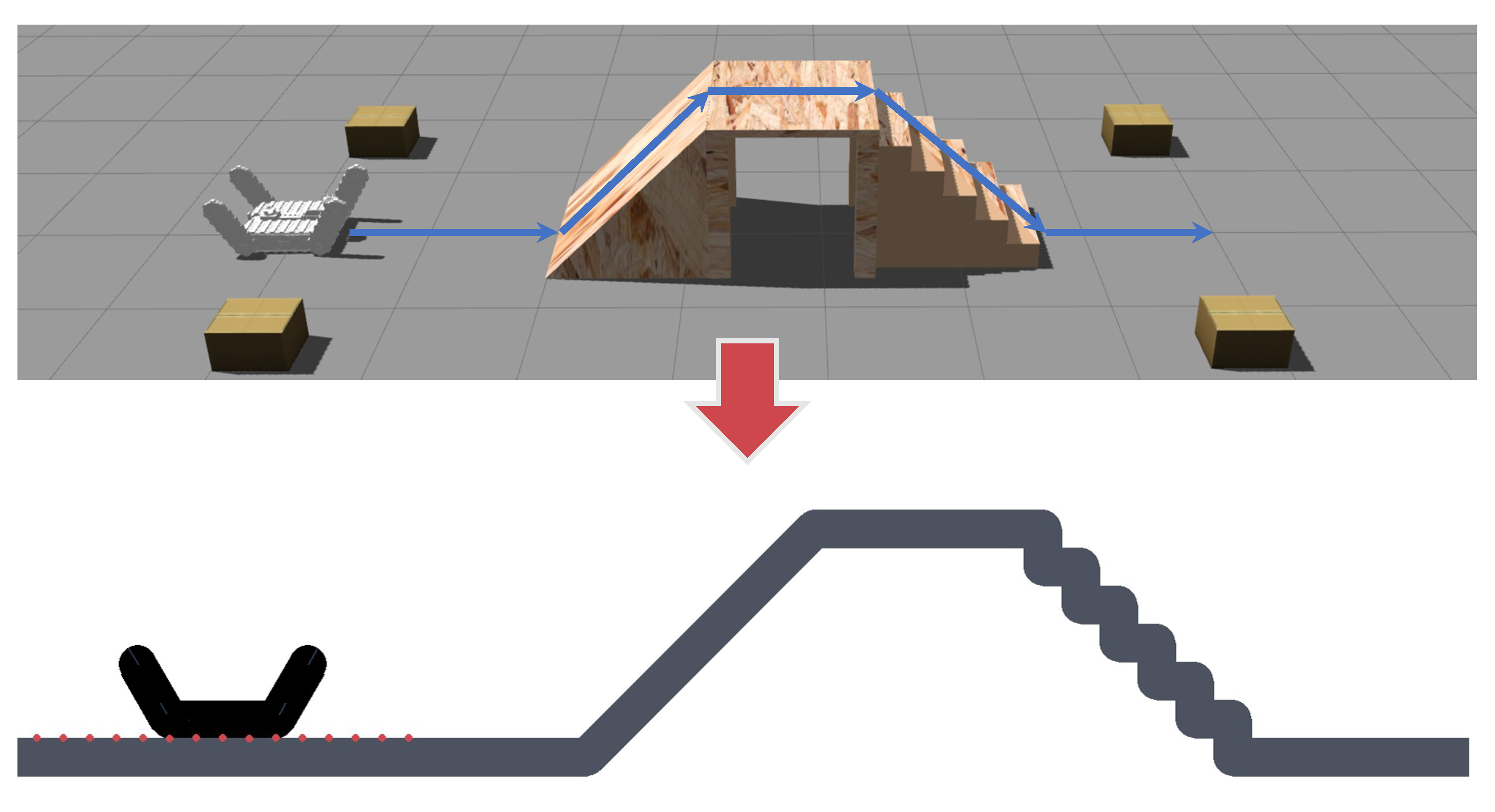
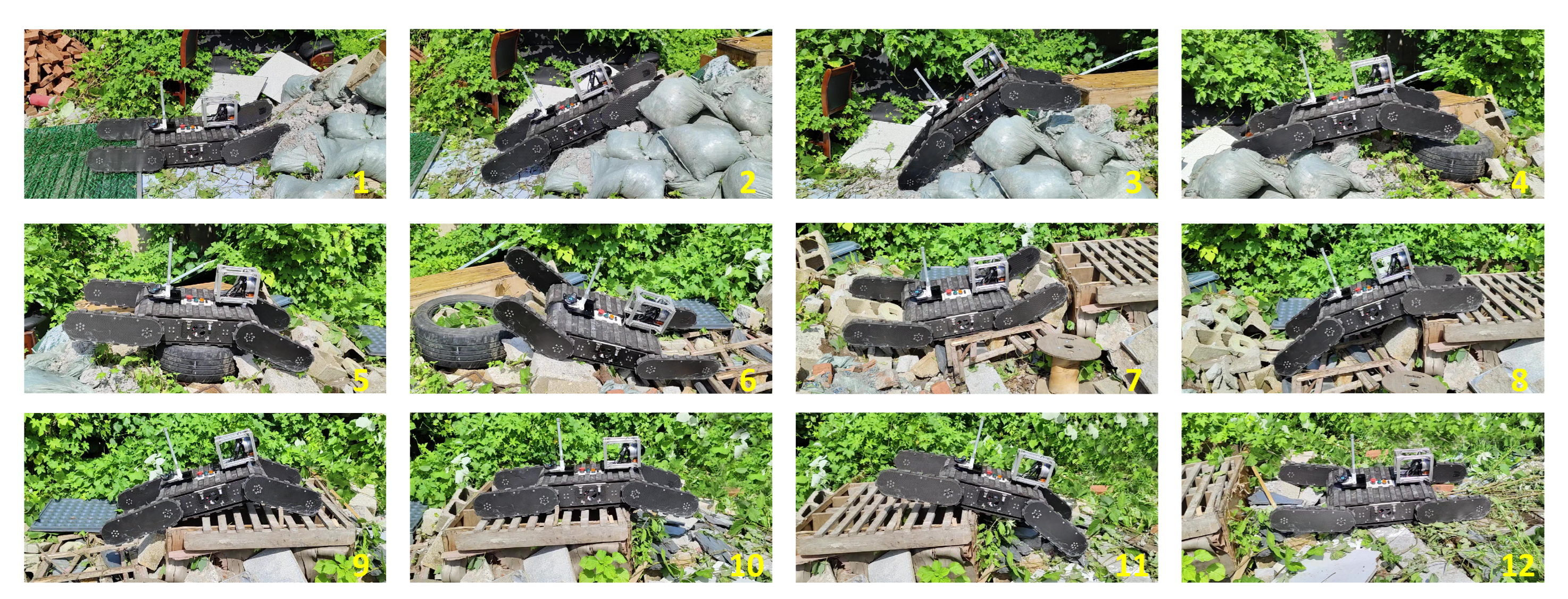
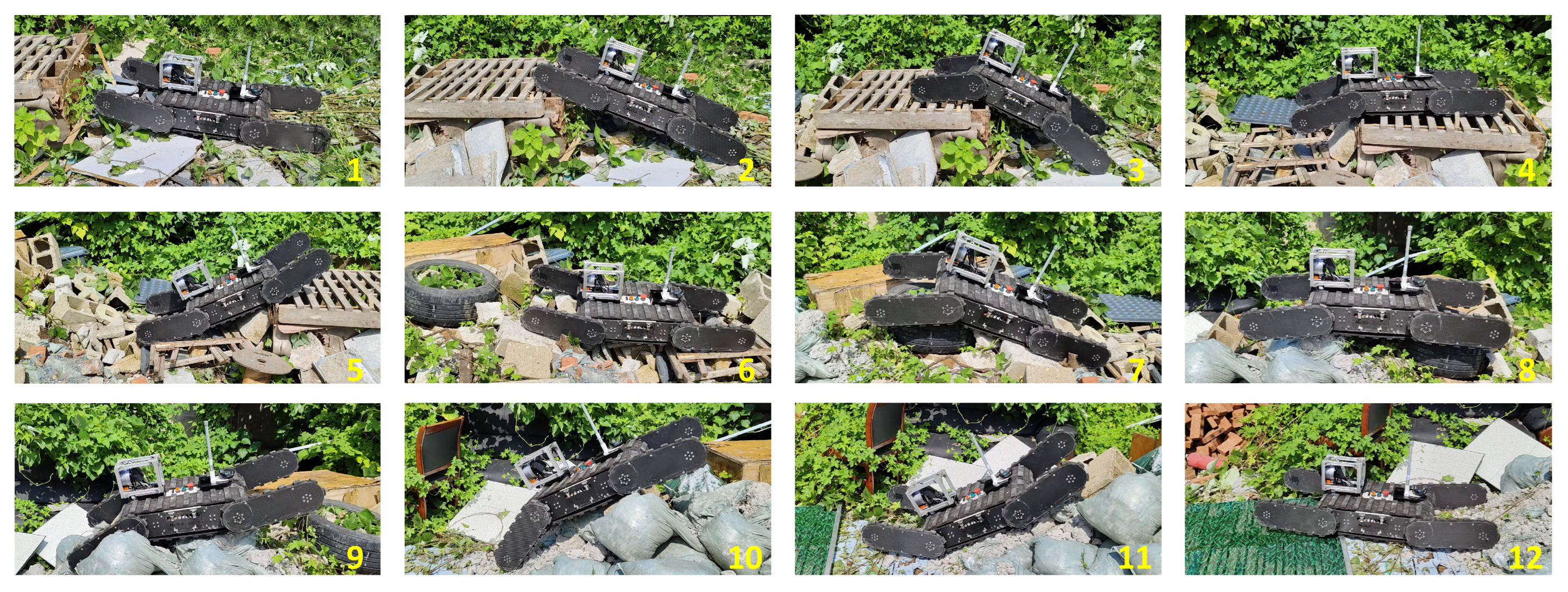
We employ our self-designed NuBot-Rescue robot as the experimental platform, as shown in
Figure 1. This platform offers advantageous central symmetry properties, and its components, namely the tracks and flippers, can be controlled independently. In this study, we assume that human operators or path-planning algorithms are responsible for controlling the rotation of the robot tracks, while the developed autonomous flipper algorithm governs the motion of the flippers.
In real-world scenarios involving traversing complex terrains, minimizing robot instability, such as side-slipping, is important. To achieve this, human operators typically align the robot’s forward direction with the undulating terrain of obstacles [
27], employing similar measures for both the left and right flippers. Building upon this premise, we project the terrain outline and robot shape onto the robot’s lateral side. An example of the robot’s and terrain interaction is shown in
Figure 2. Our approach suits environments with minor left-to-right fluctuations and significant up-and-down fluctuations.
In this article, we use DRL to develop an autonomous control system for the flippers of a tracked robot. Specifically, we formulate the problem as a Markov Decision Processes (MDP) model that leverages the robot’s current pose and surrounding terrain data as the state space (see
Section 3.2) and the front and rear flipper angles as the action space (see
Section 3.3). A reward function is established to meet the task’s particular requirements (see
Section 3.4), and subsequently, the ICM algorithm (see
Section 3.5) and a novel DRL network are introduced into the MDP model (see
Section 3.6).
3.2. State Space
Local Terrain Information H: The reference coordinate system for local terrain information
H is denoted as
. In this coordinate, the center of the robot chassis serves as the origin, with the X-axis representing the robot’s forward direction and the Z-axis indicating the opposite direction of gravity. To effectively express the Robot Terrain Interaction (RTI), we divide the point set
consisting of terrain point clouds
in front of, behind, and below the robot into N equally spaced subpoint sets
, and obtain N average heights
as local terrain information representation by downsampling (as shown by the red dots in the
Figure 3):
where
and
represent the horizontal and vertical coordinates of terrain points in the coordinate system
.
and
represent the boundaries of the perception domain along the X-axis and cover a range of
.
Figure 3 depicts the average height
within subpoint set
.
Robot State E: The coordinate system for the rescue robot is defined as an
coordinate system with the center of the robot chassis as the origin, the X-axis facing the chassis, and the Z-axis perpendicular to the chassis facing upward, as shown in
Figure 3 denoted as blue. The robot state
E consists of the angle of the robot’s front flipper
, the angle of the robot’s rear flipper
, and the chassis pitch angle
. The angle of the flipper is the X-axis angle between the flipper and the robot
coordinate system, which is positive if the flipper is above the chassis. The elevation angle of the chassis is the angle between the
coordinate system and the X-axis of the
coordinate system, which is positive if the chassis is above the X-axis of the
coordinate system.
3.4. Reward Function
A well-designed reward function is crucial in accomplishing specific tasks for robots [
28], as it encourages learning efficient control strategies for the flippers. We merge prior knowledge from human operational experts with quantitative metrics to design reward functions for RTI that satisfy the requirements for smooth and safe obstacle crossing. Specifically, a front flipper motion reward
, a smoothness reward
, and a contact stability reward
are included.
Reward of flipper : The front flipper of the robot plays a crucial role in adjusting its posture while enabling the main track to conform to the terrain as much as possible, and it needs to anticipate upcoming obstacles. We refined the practical flipper strategy based on the manual teleoperation experience introduced by Okada et al. [
8] and designed a motion-based reward function specifically for the front flipper. We denote the reward of front flippers as
.
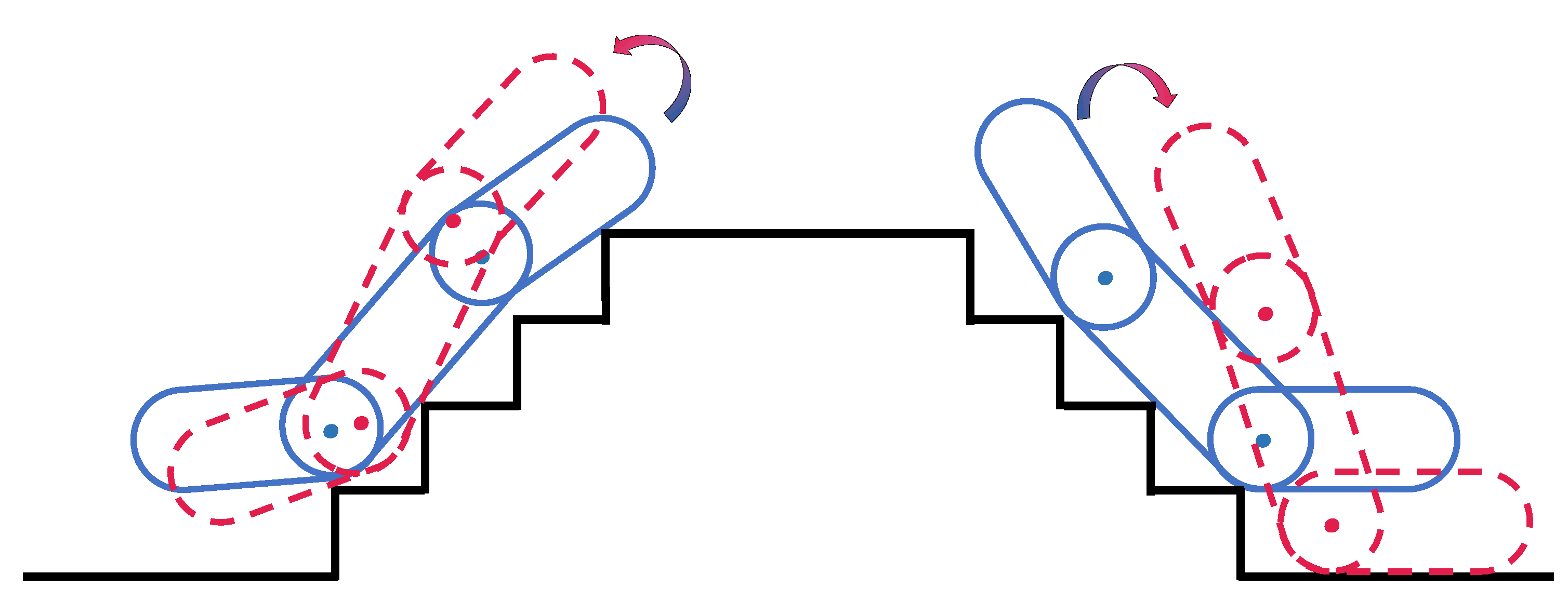
Figure 4a,b are schematic diagrams of the reward design of the front flipper when the robot goes up and down obstacles, respectively. In this section, the hinge point
between the front flipper and the chassis is selected as the reference point, which is connected with the expanded terrain point (obtained by the original terrain point expanding the half of thickness
B of the robot, shown as the red triangle) in the point set
as the vector
(shown as the green vector), and the angle between
and the X-axis of robot coordinate system are calculated. The one with the largest angle value is selected as the candidate angle of the front flipper (shown by the yellow vector). The
is mainly responsible for guiding the robot to change its posture to adapt to the terrain actively. A proper reward value is conducive to reducing the little and meaningless action exploration of the robot during training and guiding the robot to explore the reasonable front flipper action more efficiently. The absolute difference
between the robot’s front flipper angle
and the candidate angle
is taken as the reward index, and
is defined as
where
is the threshold coefficient of
.
Reward of Smoothness : Terrain traversal smoothness is an important evaluation standard, and the pitch angle of the robot chassis changes as gently as possible through the cooperation of the rear and front flippers. We propose to use the relevant indicators of the robot chassis pitch angle as a reward to optimize the robot’s terrain traversal stability, denoted as .
The absolute change in pitch angle is
, and the average change in pitch angle in
k time steps is defined as
:
where
t represents the number of steps the robot performs in a single terrain traversal episode, as shown in
Figure 5; the absolute change in pitch angle
reflects that the pitch change trend of the robot chassis is rising (
), and we limit the situation that the robot is near the overturning boundary, hoping that the pitching trend of the robot will not rise further when it is in high overturning risk. The average change in pitch angle within
k step
reflects the stability of the robot’s terrain traversal. According to the two related indexes of pitch angle mentioned above, the reward of terrain traversal smoothness is designed as
, which is defined as
where
is the threshold coefficient of
.
Reward of Contact : Under the guidance of
and
rewards, the robot can learn smooth obstacle-crossing maneuvers, but the robot’s interaction with the terrain still suffers from some implausible morphology, such as the front and rear flippers supporting the chassis off the ground. This morphology meets the smoothness constraints, but the driving force could be utilized more efficiently, and the torque applied to the flippers needs to be bigger. The contact between the tracks and the terrain is the medium of the robot’s driving force. The robot’s chassis and flippers are equipped with main and subtracks, respectively, and the size of their contact area with the terrain determines the robot’s driving ability, especially the main tracks. Therefore, the
reward needs to guide the robot to contact the terrain as much as possible with the chassis tracks to provide sufficient driving force, and there must be contact points at the front and back of the robot’s center of mass at the same time.
among them,
and
are the farthest contact points between the robot and the terrain; the partitions of
,
,
,
are shown in
Figure 4a.
Reward of Terminate : In the training process of the RL algorithm, the process from the starting point until the robot meets the end condition is called a terrain traversal episode, and a settlement reward will be given at the end of each episode. When the robot reaches the finish line smoothly, and the chassis is close to the ground, it is regarded as a successful obstacle crossing in this episode, and a big positive reward is obtained. It is necessary to design negative rewards according to the task scene’s specific situation to restrain the robot’s dangerous or inappropriate behavior. Thus, when the robot meets the following conditions, it obtains a larger settlement reward and ends the current episode:
among them,
represents the maximum number of steps the robot performs in a single terrain traversal episode, and
R represents the value of the settlement reward.
In summary, the sum of rewards
earned by the robot at each obstacle-crossing time
t is expressed as Equation (
10), where
is the weight of each reward term and
.
3.5. ICM Algorithm
To improve the robot’s exploration of obstacle-crossing action and state, ICM is designed to encourage the robot to try new actions and move to a new state so that it is possible to explore higher-reward obstacle-crossing performance. For the single-step trajectory
of MDP, ICM is used to evaluate the curiosity level of the robot in the current state. The specific structure is shown in
Figure 6, including the Encoder model, Forward prediction model, and Inverse prediction model.
Encoder model : Responsible for coding the original state space into a feature space with stronger representation ability. As the key feature state of the obstacle-crossing problem, this feature space should fully contain all the information robots use for decision making. The state space of the traversal MDP model is composed of robot state and terrain information, which fully represents the process of RTI. Encoder model is used to encode current state and transition state into feature vectors and .
Forward prediction model F: The
F simulates the operation mode of the environmental model and is used to estimate and predict the transfer characteristic state of the robot after acting. Its inputs are robot action
and characteristic state vector
, and the predicted transferred characteristic state vector
is the output. The difference between the
output by the
F and the characteristic state
encoded by the encoder
indicates the curiosity level of the robot. We introduce the curiosity level as the intrinsic reward
into the reward function of Reinforcement Learning to encourage robots to explore more unknown states. Thus, the loss function
of the
F, the intrinsic curiosity reward
, and the reward sum of each obstacle-crossing time step
can be defined as
where
,
is the scaling factor of intrinsic curiosity reward, and
M is the characteristic state vector
.
Inverse prediction model I: The core of the
I is to infer what actions the robot has taken to cause this transfer through the current and transfer states. Its inputs are the current feature state
and the transition feature state
, and the goal is to output the reasoning action
, which is as small as possible from the action
executed by the robot. Under the constraint of the backward inference model, the encoder
learns how to extract the accurate feature state space when the network is updated, thus predicting the forward inference model more accurately. The cross-entropy loss function is used to describe the loss of the
I, which can be expressed as
where
;
and
represent the probability, receptively, that the front flipper samples the
i action and the rear flipper samples the
j action in the vector
and
.
At the beginning of the algorithm, the feature extraction ability of the encoder and the prediction ability of the
F are weak; so, the curiosity value will be large, which drives the robot to explore more. With the progress of obstacle-crossing training, the state of the robot is being explored more and more, and the role of curiosity mechanisms in encouraging exploration will gradually decrease, making the robot make more use of learned action strategies. To sum up, the overall loss function of the ICM algorithm is expressed as follows:
where
and
are the coefficients of forward prediction model loss and backward inference model loss, and
and
are the network parameters of ICM.
3.6. Algorithm and Network
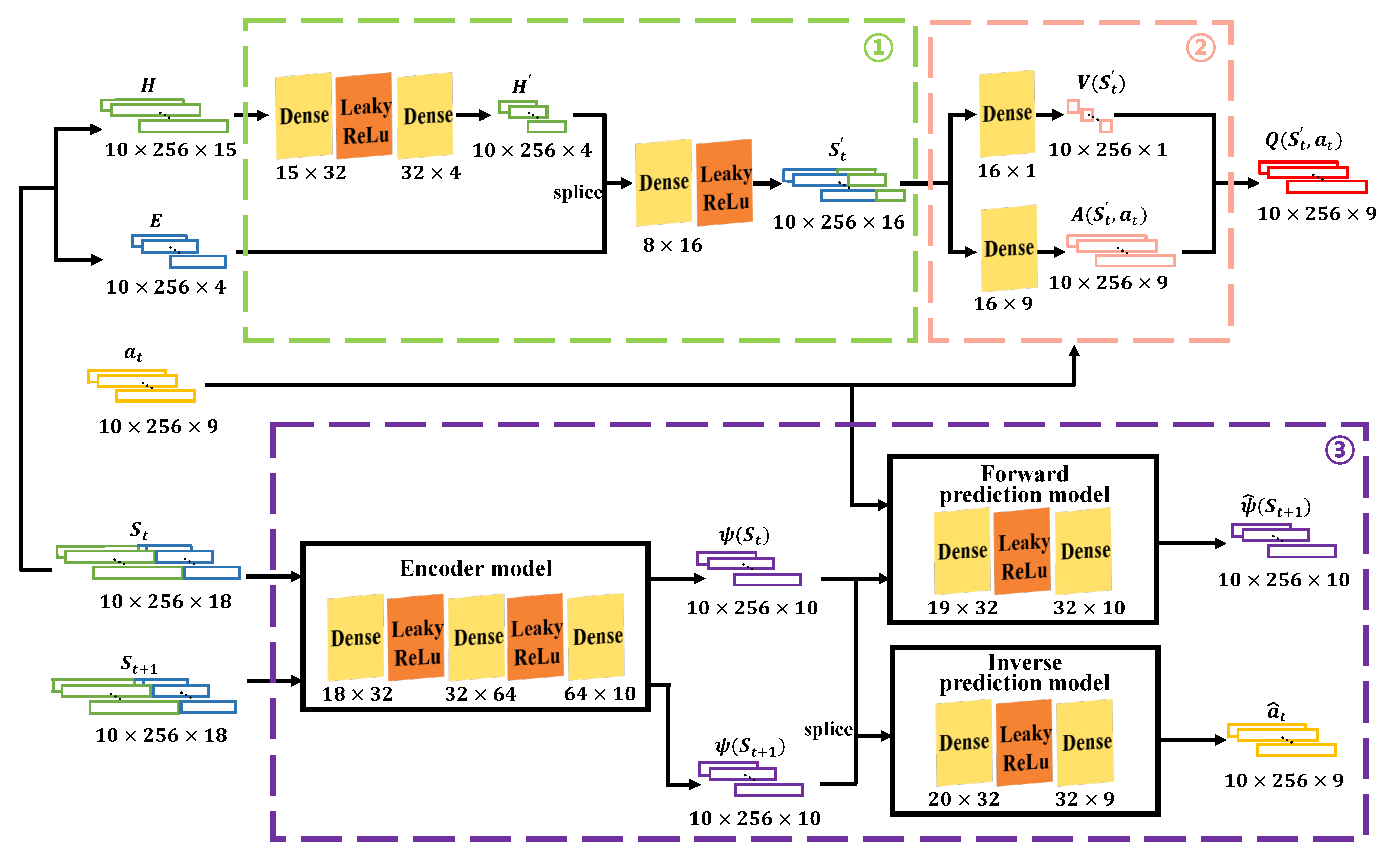
We show our DRL network architecture in
Figure 7, which consists of three main blocks. The block ① highlighted in green is the RTI feature extraction module, which is responsible for generating the interaction features during the terrain traversal process. Terrain data
H (green vector) and robot information
E (blue vector) are fed into the network to produce the interaction feature vector
via the front-end feature extraction module. Due to the relatively small size of the estimated motion vectors, robot state, and terrain information, there is no requirement for designing complex networks similar to those used for images or 3D point clouds [
29]. The network mainly consists of fully connected layers (yellow) and LeakyReLu nonlinear activation layers (orange). Multilayer Perceptron (MLP) is employed to extract features from terrain information
, incorporating them with robot state information
E to create a new interactive feature vector
through single-layer MLP.
The block ② highlighted in orange is the D3QN module, which combines the advantages of Double DQN [
30] and Dueling DQN [
31]. D3QN uses the advantage function
to evaluate the relative value of each action in the current state to help the robot make more informed decisions. The
is calculated by subtracting the state value function
from the action value function
(the output of the Q network). Specifically, the
is used to estimate the expected return in a given state, which is to evaluate the value of the
. The
is used to estimate the expected return of taking a specific action in a given state, which is to evaluate the value of action
. By calculating the
, we can obtain the potential of each action relative to the average level in the current state, and the robot can choose the action with the greatest advantage to execute, thus improving the accuracy and effect of decision making.
The block ③ highlighted in purple is the ICM network, which is responsible for outputting the intrinsic reward. The network structure of its Encoder model , Forward prediction model F, and Inverse prediction model I consists of 3, 2, and 2 MLP layers, respectively.

