Article

Multi-Factor Collaborative Analysis of Conservation Effectiveness of Nature Reserves Based on Remote Sensing Data and Google Earth Engine

1
School of Forestry, Northeast Forestry University, Harbin 150040, China
2
Key Laboratory of Sustainable Forest Ecosystem Management-Ministry of Education, Northeast Forestry University, Harbin 150040, China
3
College of Geomatics, Xi’an University of Science and Technology, Xi’an 710054, China
*
Author to whom correspondence should be addressed.
Remote Sens. 2023, 15(18), 4594; https://doi.org/10.3390/rs15184594
Submission received: 27 July 2023 / Revised: 16 September 2023 / Accepted: 17 September 2023 / Published: 18 September 2023

Abstract

:
Protected areas (PAs) play a crucial role in safeguarding biological resources and preserving ecosystems. However, the lack of standardized and highly operational criteria for evaluating their conservation effectiveness, particularly across different ecological types, remains a significant gap in the literature. This study aims to address this gap by constructing a conservation effectiveness evaluation model for two distinct types of PAs in Heilongjiang Province, China: the Zhalong National Nature Reserve (ZlNNR), a wetland ecological reserve; and the Mudanfeng National Nature Reserve (MdfNNR), a forest ecological reserve. We employed various methods, including land use dynamic index, visual analysis of landscape patterns, remote sensing inversion, and a multi-factor comprehensive assessment model, to assess changes in conservation effectiveness from 2000 to 2020. Our findings reveal a contrast between the two PAs. In the ZlNNR, croplands and water bodies increased significantly by 4069.4 ha (K = 1.5820%) and 2541.58 ha (K = 3.2692%). In the MdfNNR, impervious lands increased greatly by 65.35 ha (K = 7.4021%), whereas forest lands decreased by 125 ha (K = −0.067%). The core area of the two PAs displayed increased landscape regularity, whereas the experimental area showed heightened landscape diversity. In ZlNNR, the MPSL value increased by 134.91%, whereas the PDL value decreased by 57.43%, indicating a more regular landscape pattern. In MdfNNR, the SHDIL value decreased by 110.7%, whereas the PDL value increased by 52.55%, indicating a more fragmented landscape pattern. The area with improved vegetation trends in ZlNNR was 8.59% larger than in MdfNNR, whereas the area with degraded vegetation trends was 4.86% smaller than in MdfNNR. In all years, the high effectiveness area was larger in ZlNNR than in MdfNNR, whereas the medium and low effectiveness areas were smaller in ZlNNR compared to MdfNNR. This study provides a scientifically rigorous assessment method for evaluating the conservation effectiveness of different types of PAs, laying a solid theoretical foundation and practical guidance for future conservation strategies.

Graphical Abstract

1. Introduction

Protected areas (PAs), as delineated in scholarly literature, are unique geographical zones that are not only legally recognized and managed, but are also committed to the enduring preservation of nature, inclusive of the associated ecosystem services and cultural values [1]. At present, the establishment of PAs is a pivotal global strategy for biodiversity conservation, climate change mitigation, and the reduction of human impact [2,3,4,5,6,7]. It also serves as a significant policy instrument for the protection of natural resources and the promotion of sustainable development [1,8,9]. China, being one of the countries with the most diverse ecosystems globally, has instituted more than ten categories of PAs, which encompass 18% of its terrestrial area and 4.1% of its marine area [10,11,12]. However, numerous PAs are still under considerable pressure, confronting challenges such as the exploitation of agricultural and forestry products, illegal hunting, and infrastructure development [13]. In essence, merely augmenting the quantity and size of PAs is no longer adequate to cater to the present and future requirements of biodiversity conservation [12,14]. The most pressing concern at this juncture is to amplify the effectiveness of existing PAs to ensure their preservation [15].
The effectiveness of PAs is contingent on a multitude of political, economic, and local environmental factors. There are authoritative domestic and international assessment standards for PAs, such as the Standard for Conservation Effectiveness Assessment of Ecology and Environment in Nature Reserves, promulgated by the Ministry of Ecology and Environment of China, and Evaluating Effectiveness: A Framework for Assessing Management Effectiveness of Protected Areas, published by the International Union for Conservation of Nature (IUCN), Gland, Switzerland. In practice, the assessment criteria are relatively sophisticated, necessitating specialized technical expertise, rendering implementation challenging. Furthermore, numerous studies have utilized multi-temporal historical land use data to appraise the land use/land cover changes and landscape pattern dynamics within PAs [16,17,18]. Indexes such as the landscape development intensity index and landscape pressure index have been employed by academics to assess the effectiveness of safeguarding marine PAs [19]. In addition, alterations in ecosystems, as well as the distribution and abundance of key species, also serve as indicators of conservation effectiveness [20,21,22]. Nevertheless, these existing evaluation techniques are often labor-intensive and time-consuming [23,24], or necessitate plenty of field investigations [21].
Remote Sensing (RS) is an advanced data acquisition technology that can swiftly, comprehensively, and accurately generate thematic data. It facilitates repeated observations of large territories and inaccessible areas, proving to be more cost-effective than field observations [25,26]. In recent years, research using satellite imagery to predict sustainable development outcomes has achieved rapid growth, especially studies employing machine learning methods. Satellite data with greatly improved spatial, temporal, and spectral resolutions have provided richer information on the Earth’s surface. RS meets the needs for monitoring sustainable development outcomes, with the advantages of mature technology, rapid data updates, and extensive coverage, which can satisfy the requirements of large-scale, high-precision effectiveness monitoring in PAs [27]. The Geographic Information System (GIS), with its robust information extraction technology and spatial analysis capabilities, can accurately and efficiently address geographic issues related to resources and the environment [28]. The significance of this technology continues to escalate, with ongoing enhancements to its role and functionality. Consequently, the integration of RS and GIS has emerged as the preferred methodology for evaluating the conservation effectiveness of PAs.
From our perspective of PAs as habitats for various species, the quality trends, whether improving or deteriorating, are an important reflection of the changing effectiveness of conservation efforts. We utilize an integrated approach of RS and GIS techniques to conduct monitoring of PA quality changes. This allows for more cost-effective and extensive spatio-temporal analyses compared to conventional methods based on localized ground surveys. Furthermore, our multi-factorial integrated assessment model employs a weighted summation method, which can effectively mitigate the limitations of single-factor evaluation lacking accuracy. This represents a methodological innovation in our research. These represent the innovations in our research ideology and analytical methodology. Thus far, many appraisals of conservation effectiveness have focused solely on either a single category of PA [21,29] or involved a plethora of disparate PA categories [19,30,31,32,33,34]. Therefore, our study aims to analyze differences in the effects of various PA types through a comparative analysis of two major types (forest and wetland PAs). By concentrating the analysis on these two predominant habitat types, we can gain deeper insights into the relative performance of PAs designated for forests versus wetlands in terms of conservation outcomes and effectiveness.
Land use change is a pivotal factor driving global environmental change [35,36]. It provides a direct perspective on the impact of human activities on surface ecosystems [37], effectively mirroring the ecosystem status of PAs [38]. Landscape pattern serves as a vital means to depict landscape structure [39]. Landscape indexes encapsulate essential information about landscape patterns, and can serve as macro-scale surrogate indicators to perceive and comprehend changes in species and their habitats [21]. Landscape indexes have been extensively employed to assess the effectiveness of PAs [40,41,42]. The spatial and temporal variation of the Normalized Difference Vegetation Index (NDVI) is one of the most cost-effective methods for assessing ecological effectiveness [34,43,44,45]. The Google Earth Engine (GEE) Cloud Platform can swiftly and accurately process remote sensing images using its robust data calculation function. It can also obtain the best-quality images through minimum cloud amount screening for research [46,47,48], thereby yielding the results of time series changes of NDVI. Consequently, employing the aforementioned factors to evaluate the effectiveness of PAs in a more systematic manner holds significant guiding implications.
Frequently, forests are often referred to as the “lungs of the earth”, playing a pivotal role in the global carbon cycle, regulating the climate system, and protecting biodiversity [49,50,51,52]. Wetlands, on the other hand, are commonly referred to as the “kidney of the earth”, providing a habitat for a vast array of species [53], maintaining the ecological balance [54,55,56], and mitigating the impact of extreme weather and other outside destructive forces on surrounding areas [57]. Both ecosystems are critically important, yet are under severe threat [51,53]. The establishment of forest ecosystem PAs and wetland ecosystem PAs is a key approach to protecting forests and wetlands, and a universally powerful tool to reverse the rapid imbalance and degradation of these two ecosystems [58]. Given disparities in the developmental status and geographic contexts of these two PA types, they may encounter differing degrees of threat and exhibit variations in biodiversity composition and structure [30]. Consequently, their responses and outcomes regarding conservation management could diverge as well. Therefore, to what extent do differences exist in the conservation effectiveness between these two types of PAs? What are the driving factors contributing to these differences? Through comparison, we can ascertain relative superiority in habitat quality conservation outcomes, elucidate the adaptive propriety of conservation management across contrasting ecosystems, and evaluate the necessity of establishing specialized PAs grounded in particular ecological systems.
In light of the above, the objectives of this study are delineated into the following components: (1) the development of a conservation effectiveness evaluation model that incorporates parameters such as land use, landscape pattern, and NDVI; (2) the exploration of the differences in conservation effectiveness between Zhalong National Nature Reserve (ZlNNR), Qiqihaer, China and Mudanfeng National Nature Reserve (MdfNNR), Mudanjiang, China from the period of 2000 to 2020; (3) the identification of the primary driving factors influencing the conservation effectiveness of each PA, and the provision of scientifically sound and reasonable suggestions for the effective management of PAs.

2. Materials and Methods

2.1. Study Areas

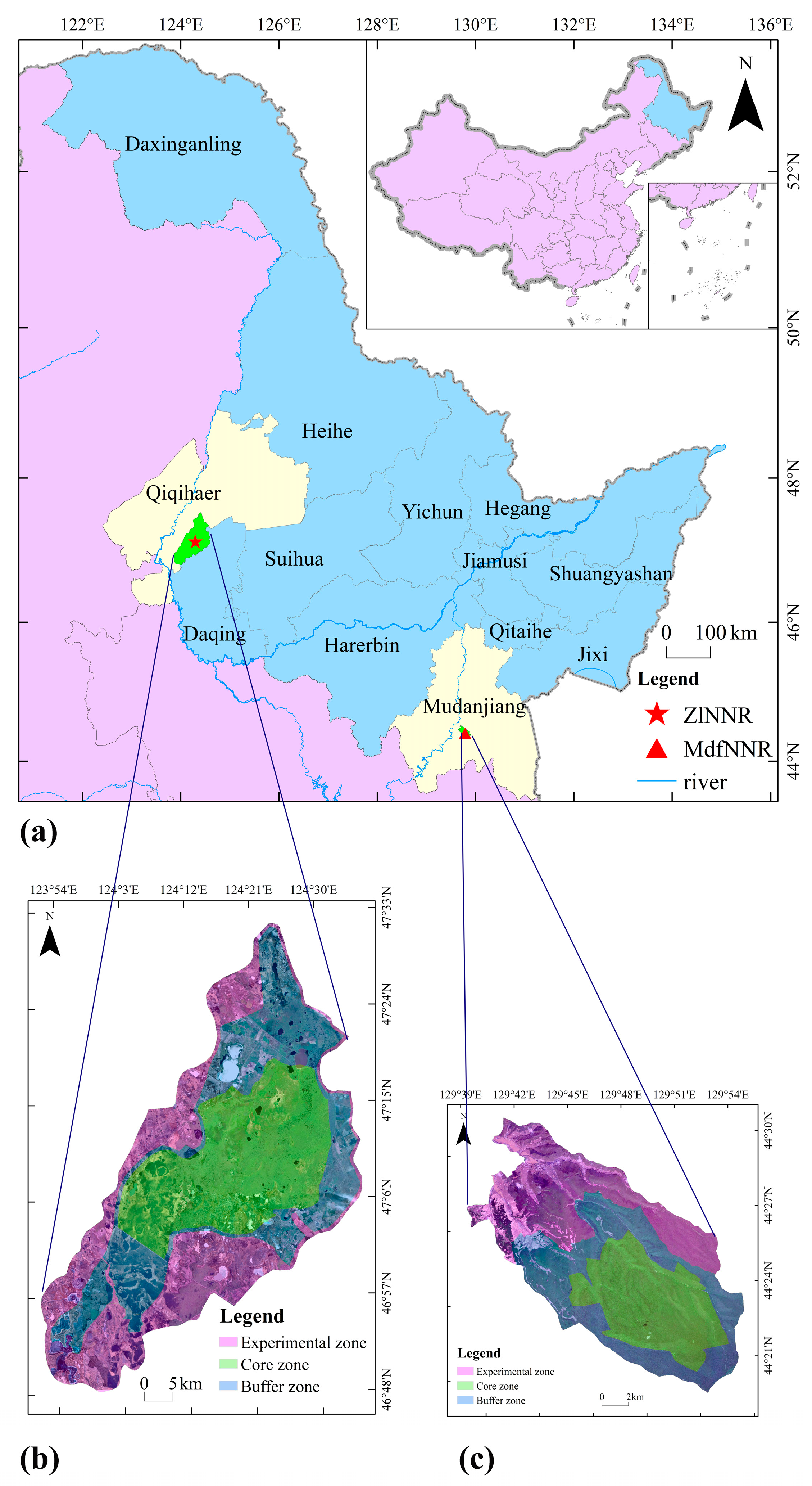
The ZlNNR study area is situated in the Songnen Plain in the west of Heilongjiang Province, southeast of Qiqihar City (Figure 1), within the reed marsh belt in the lower reaches of the Wuyuer River. It belongs to the wetland ecosystem type, and focuses on protecting rare bird species such as red-crowned cranes and wetland ecosystems [59,60]. It is the most complete, primitive, and open wetland ecosystem in the same latitude area of northern China [61]. The reserve, irregularly shaped like an olive and stretching from northeast to southwest, spans a total area of 2100 km2. Its geographical coordinates are 123°47′~124°37′E and 46°52′~47°32′N. The region experiences a temperate continental monsoon climate, with an annual average temperature of 2~4 °C, annual precipitation of approximately 426 mm, and annual evaporation of 1307.7 mm [61,62].
The MdfNNR study area is located in the low-altitude Laoyeling mountains, southeast of Mudanjiang City (Figure 1), and is 15 km away from the city center [63]. It is a forest ecosystem, covering a total area of 210 km2, with geographical coordinates of 129°40′~129°53′E and 44°20′~44°30′N. The region is characterized by a temperate continental monsoon climate, featuring dry and windy springs, followed by warm and wet summers. The average annual temperature is a moderate 3.6 °C, whereas the annual precipitation averages at 550 mm. The majority of this precipitation occurs during the growing season, which typically spans from June to August [64].
Both the NNR and buffer (ZlNNR: 10-km-wide, MdfNNR: 3-km-wide) around them are the concerned areas in this paper.

2.2. Data Sources

In this study, land cover/land use data were derived from the GlobeLand30 data platform [65,66,67]. These maps have recently been considered useful references for land use studies and have been used to classify land use [68]. The remote sensing image data use the GEE platform programming (JavaScript API) [69] to call the Landsat-5 TM, Landsat-7 ETM+, and Landsat-8 OLI surface reflection data set to screen the cloud amount of the whole year’s image. A total of 2012 available Landsat images were obtained across the two PAs and their surroundings. The images are then mosaicked to find the minimum cloud cover image of the research area from 2000 to 2020. Notably, since the Landsat-5 data set only contains the images from 2003 to 2011, and the Landsat-7 satellite failed in 2003, images after that year cannot be used and the images from 2012 are discarded during the analysis.

2.3. Method

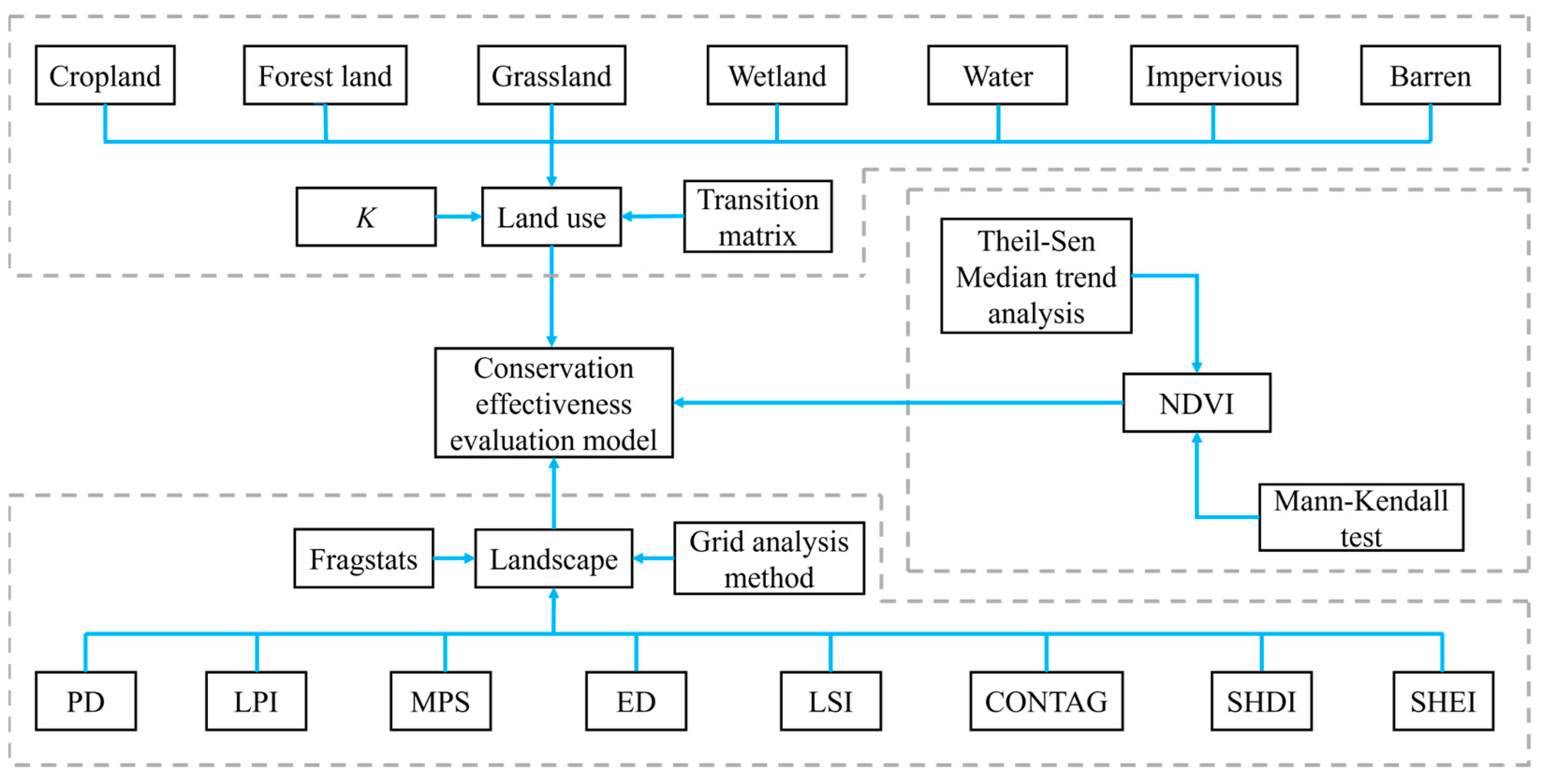
Figure 2 shows the specific processes of assessing the conservation effectiveness and the included indexes.

2.3.1. Land Use Change

The analysis of land use change is conducted from two perspectives: temporal series variation and differences inside and outside PAs. The ArcGIS 10.8 software (ESRI (Environmental Systems Research Institute). 2018. ArcGIS Desktop: Release 10.8. Redlands, CA, USA: Environmental Systems Research Institute. https://www.esri.com/en-us/arcgis/products/arcgis-desktop/overview, accessed on 9 April 2023) is used to make statistics on the land use area and transfer matrix characteristics to analyze the process and degree of change among different land use types in the study areas. The dynamic degree model of land use is used to analyze the change degree of various types of land use [21,70,71]. The dynamic degree index (K) is calculated as follows:
K = U a U b U b × 1 T × 100 %
where, K refers to the dynamic degree of a certain land use type during the study period; Ub and Ua are the areas of a certain land use type before and after the study period, respectively (unit: ha); and T is the number of years between the study period.

2.3.2. Landscape Pattern

The landscape pattern index value can effectively encapsulate information pertaining to landscape development. It can accurately reflect the composition and dynamic changes of the landscape structure, and closely aligns spatial changes of the landscape with the temporal process [72]. In this study, eight indexes were selected from the patch level and landscape level to analyze the changes in landscape pattern, referencing previous studies. Additionally, these indexes at the patch level were categorized into two groups: patch characteristics and patch shape. At the landscape level, they were divided into three categories: landscape characteristics, landscape shape, and landscape diversity [73]. The calculation formula for each index is presented in Table 1. The grid analysis method was employed to visually analyze the landscape level of the landscape pattern indexes of both NNRs. Primarily, referring to the relevant literature [74,75,76,77], considering the area and scale of each study area, ZlNNR and MdfNNR were divided into 2 km × 2 km and 0.5 km × 0.5 km grid cells, respectively. Furthermore, the landscape indexes of each study area were interpolated and analyzed using the Kriging interpolation method.

2.3.3. Trend Analysis of NDVI

NDVI is suitable for characterizing the growth and spatial distribution of vegetation within our study area [82,83]. We extracted the annual average NDVI value for each pixel within the study areas through the GEE platform [84,85]. However, when conducting a univariate analysis of NDVI, there are several considerations that must be taken into account. NDVI may exhibit anomalous values in non-vegetated regions. Furthermore, water bodies result in negative NDVI values. Therefore, when performing an isolated NDVI analysis, croplands, water bodies, barren areas, and impervious areas were excluded from the study areas. This was done to avoid potentially skewed results arising from these land cover types which do not accurately represent vegetation dynamics. The time series analysis of NDVI was conducted pixel by pixel using the Theil–Sen median trend analysis [86,87] and Mann–Kendall trend test [88,89]. The Theil–Sen Median method is a robust non-parametric statistical trend calculation method. This method boasts high computational efficiency, is insensitive to measurement errors and clustered data, and is apt for the trend analysis of long-term series data. The Mann–Kendall test is a non-parametric time series trend test method, which does not require measurement values to conform to a normal distribution and is unaffected by missing values and outliers. It is suitable for the trend significance test of long-time series data. Both methods are vital for determining the trend of long-time series data and can be effectively combined. This combination has gradually been used to analyze and reflect the trend change of each pixel in the long-time series [84,90,91,92,93].
The calculation formula of NDVI is:
N D V I = N I R R N I R + R
where NIR refers to near-infrared band value. R represents red band value.
The calculation formula of the Theil–Sen median method is:
β = M e d i a n ( N D V I j N D V I i j i ) , j > i
where Median() represents the median value, and NDVIi and NDVIj represent the NDVI values in years i and j. If β > 0, the NDVI is on an upward trend; otherwise, it is a downward trend.
The calculation formula of the Mann–Kendall test is as follows. The calculation formula of test statistic S is:
S = i = 1 n 1 j = i + 1 n s g n ( N D V I j N D V I i )
where sgn() is a symbolic function, and the calculation formula is:
s g n ( N D V I j N D V I i ) = { + 1   N D V I j N D V I i > 0     0     N D V I j N D V I i = 0 1   N D V I j N D V I i < 0
The calculation formula of test statistic Z is:
Z = { S V a r ( S ) ( S > 0 )                 0               ( S = 0 ) S + 1 V a r ( S ) ( S < 0 )
where the formula for calculating Var is:
V a r ( S ) = n ( n 1 ) ( 2 n + 15 ) 18
where n is the length of data in the sequence.

2.3.4. Evaluation and Analysis of Conservation Effectiveness

The evaluation indicator system is presented in Table 2. We selected evaluation indicator data for the years 2000, 2010, and 2020 to conduct a comprehensive evaluation of conservation effectiveness. The weight of the secondary evaluation index was calculated first, followed by the weight of the primary evaluation index using the coefficient of variation results of the secondary evaluation index. The coefficient of variation method [93,94] was employed to determine the weight of each indicator. The formula for calculating the coefficient of variation method is:
v i = σ i / x i ¯
W i = v i / i = 1 n v i
where Wi refers to the weight of index i; vi represents the coefficient of variation of index i; σi represents the standard deviation of index i; x i ¯ is the average of index i.
We then standardized the evaluation factors between [0–10] and used the relative evaluation method to evaluate the conservation effectiveness of the NNRs [95]. The indicator data of the NNRs were collated into a database for use. According to the weight of each evaluation indicator, all evaluation indexes were spatially superimposed by the method of weighted summation to calculate the conservation effectiveness indicator of the NNRs. Subsequently, we employed an equal spacing segmentation method and divided the NNRs into three level intervals, high effectiveness (HE), medium effectiveness (ME), and low effectiveness (LE), to realize the comprehensive evaluation of the conservation effectiveness of the NNRs [96]. The model calculation formula is as follows [97]:
E = i = 1 n W i × X i
where E is the conservation effectiveness index of the study area; Xi refers to the quantitative expression value of the evaluation index i element after standardization; and n is the number of thematic index elements participating in the evaluation.

3. Results

3.1. Land Use

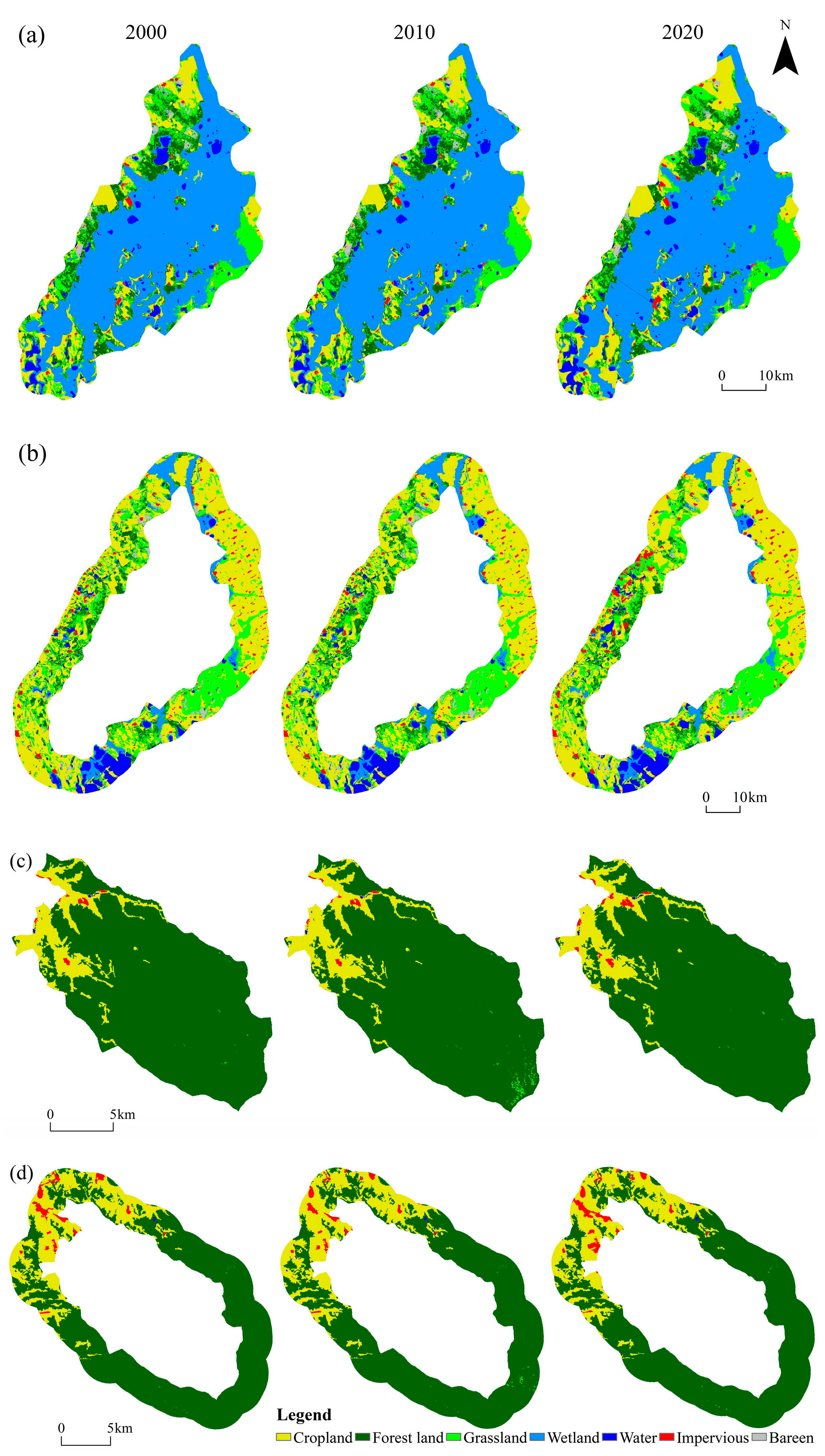
Wetland constitutes the primary land use type in ZlNNR, accounting for approximately 50% of the total area (Figure 3a and Table 3). Over the span of twenty-one years, the wetlands experienced a reduction of 5115 ha (K = −0.3998%). However, the areas of croplands and water bodies significantly increased, by 4069.4 ha (K = 1.5820%) and 2541.58 ha (K = 3.2692%), respectively. The change in grasslands was the least significant (K = 0.2296%). Outside the NNR (Figure 3b), impervious lands (K = 5.6867%) underwent the largest change, whereas the croplands, being the primary land use type outside of ZlNNR, exhibited the smallest change range (K = 0.0036%).
A total of 25,481.16 ha and 43,366.68 ha of land underwent transformation inside and outside ZlNNR, accounting for approximately 11.94% and 17.01% of their respective total areas (Figure 4a,b). Among these, inside the ZlNNR, the area of grasslands experienced the largest transformation, with 8115.78 ha transferred out, accounting for 30.60% of the total area of grasslands, primarily converted into forest lands (3410.08 ha) and croplands (2894.82 ha). The area transferred from impervious lands was the smallest, with 285.76 ha transferred out, accounting for 16.51% of the total area of impervious lands, mainly converted into croplands (177.65 ha). Outside the ZlNNR, the area of grasslands transferred out was the largest (14,932.17 ha), accounting for 24.23% of the total grasslands area, and primarily converted into croplands (6615.25 ha). The area transferred from impervious lands was the smallest (877.59 ha), accounting for 12.98% of the total area of impervious lands, and mainly converted to croplands (577.69 ha). The area of wetlands both inside and outside of ZlNNR has declined.
Forest lands constitute the primary land use type both inside and outside of MdfNNR, covering 86.98% of the total area inside the reserve (Figure 3c,d and Table 4). Inside the MdfNNR, the area of impervious lands exhibited the largest increase of 65.35 ha (K = 7.4021%). Conversely, the area of grasslands showed the smallest increase, expanding by a mere 1.4 ha (K = 2.0871%). However, forest lands were the only land type that decreased in size, with a total reduction of 125 ha (K = −0.067%). Outside the MdfNNR, only forest lands decreased in area, with a total reduction of 232.1 ha (K = −0.1351%). The area of croplands underwent the most significant change, 138.28 ha (K = 0.2532%). The most substantial change was observed in grasslands (K = 15.8699%).
In total, 761.04 ha and 1582.36 ha of land inside and outside of MdfNNR underwent changes, accounting for approximately 3.58% and 6.85% of the total area inside and outside of the NNR, respectively (Figure 4c,d). Among these, the largest transfer inside the MdfNNR was observed in forest lands, with an area of 392.26 ha and a ratio of 2.11% of the total forest lands area, primarily converted into croplands (382.24 ha). The area of grasslands transferred was the least (5.96 ha), with a ratio of 88.54% of the total grasslands area, all of which were converted into forest lands. Outside the MdfNNR, the area of forest lands transfer was the largest (740.58 ha), with a ratio of 4.33%, which was mainly converted into croplands (690.47 ha). The grasslands contributed the smallest area change of 9.25 ha, but the largest conversion ratio of 91.03% of its total area, mainly transformed into forest lands (8.13 ha).

3.2. Landscape Pattern

The patch level of the landscape pattern indexes of both NNRs are presented in Table 5 and Table 6. There was a negligible difference in the average values of PDP inside and outside ZlNNR. Notably, the LPIP and MPSP of inside wetland patches were much larger than those of outside wetland patches. Over the past 21 years, the change extents of the three indexes were larger outside wetland patches than those of the inside wetland. Conversely, the average values of LPIP and MPSP outside were generally more dwarf than those inside, especially for forest land types, and the average value of PDP outside MdfNNR was also generally larger than that inside. The change extent of PDP and LPIP values was generally greater outside than inside in MdfNNR, whereas the change extent of MPSP value shows the opposite trend, with the extent of change in outside indexes being smaller than that of the inside. Whether in ZlNNR or MdfNNR, in terms of patch shape, the average values of EDP and LSIP are generally higher outside than inside, and the variation ranges of the two indexes were the same.
The landscape level of the landscape pattern indexes for each study area are presented in Table 7 and Table 8. Regarding the landscape characteristics, the change extent of the PDL and MPSL values was larger outside ZlNNR than inside, with the LPIL value being greater inside ZlNNR than outside. The change extent of the PDL and LPIL values outside MdfNNR was larger than inside, whereas the three-year mean of LPIL and MPSL values was smaller outside compared to inside, with PDL showing the opposite trend. As for changes in landscape shape, the four indexes demonstrate greater fluctuation outside the ZlNNR than inside, whereas the three-year mean of EDL and LSIL values was higher outside than inside, and CONTAGL was similar between inside and outside. Additionally, the change extent of the EDL and LSIL values was smaller inside MdfNNR than outside, and the three-year mean of EDL and LSIL values was higher outside than inside. Regarding landscape diversity, the change extent of the SHDIL and SHEIL values was smaller inside ZlNNR than outside, and the average values of both indexes were larger inside ZlNNR than outside, but vice versa for MdfNNR.
Comparing the patch indexes between the two PAs, we found that from 2000–2020, the PDP, LPIP, and EDP values increased in MdfNNR, with water bodies increasing the most (65.74%, 53.09%, and 53.34%, respectively). The MPSP value only increased for cropland, but the increase was small, at just 1.74%, whereas other patch types decreased. Water bodies decreased the most (56.20%). The LSIP value change was negligible. In ZlNNR, both LPIP and EDP value increased, with the LPIP value of cropland increasing the most (54.95%) and the EDP value of barren land increasing the most (62.52%). The PDP value of wetlands decreased the most (63.33%), whereas MPSP increased the most for wetlands (72.32%). The LSIP value change was also negligible. Overall, wetland and impervious surface patches became more regular in shape in ZlNNR, whereas patch types became increasingly fragmented. In MdfNNR, all patch types became increasingly fragmented, especially forest, grassland, and water body patches. For landscape index, the MPSL, CONTAGL, and SHDIL values of ZlNNR increased by 134.91%, 6.93%, and 2.76% respectively, whereas the rest of the index values decreased. Notably, the PDL value decreased by 57.43%. For MdfNNR, the MPSL, SHDIL, and SHEIL values decreased by 110.7%, 124.43%, and 101.61%, respectively, whereas the other index values increased. Notably, the PDL value increased by 52.55%. This indicates that the MdfNNR landscape became increasingly fragmented with weaker connectivity, reduced diversity, and irregularity. In contrast, the ZlNNR landscape showed smaller distribution evenness changes, enhanced connectivity, increased aggregation, and more regular shapes.
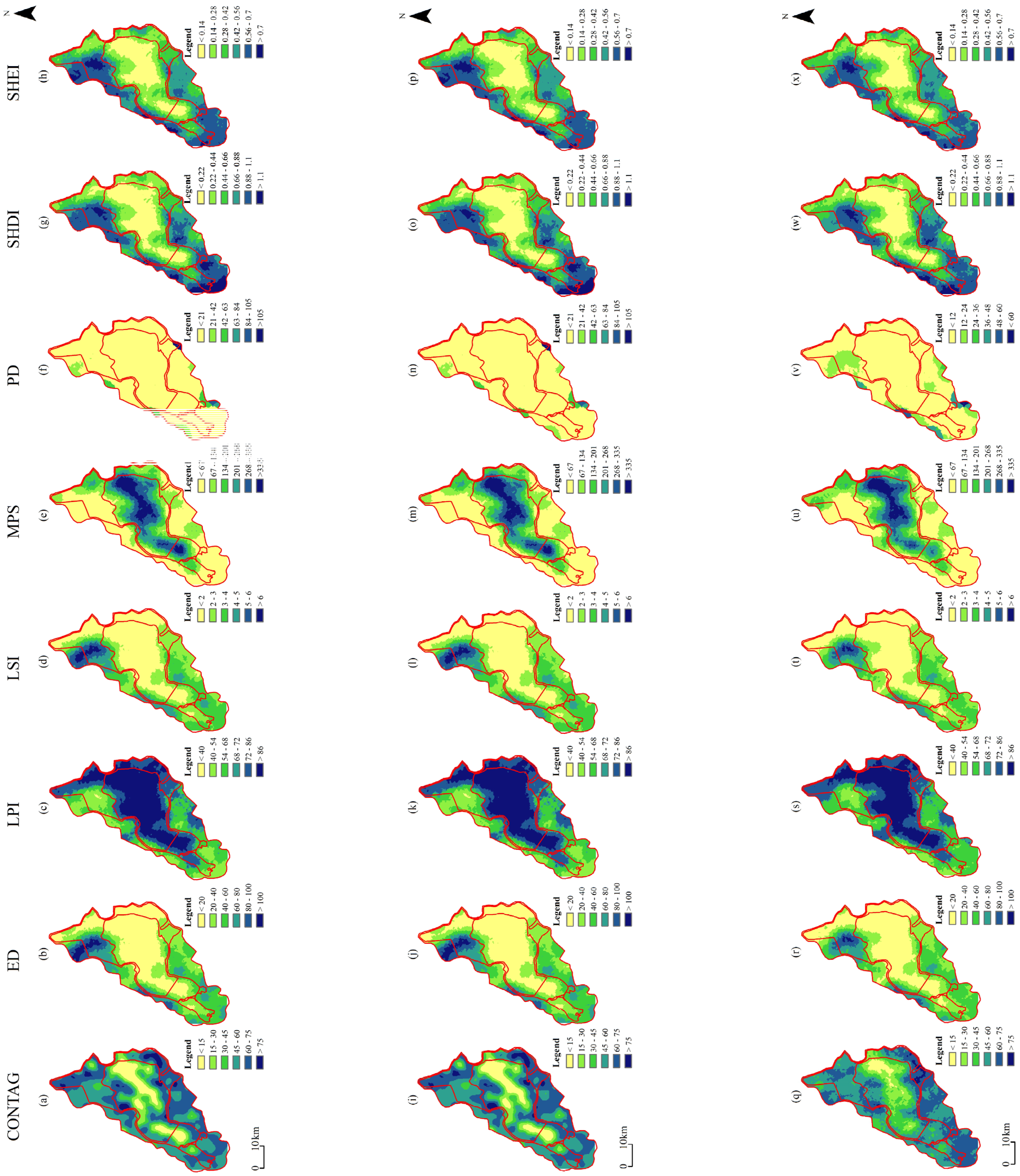
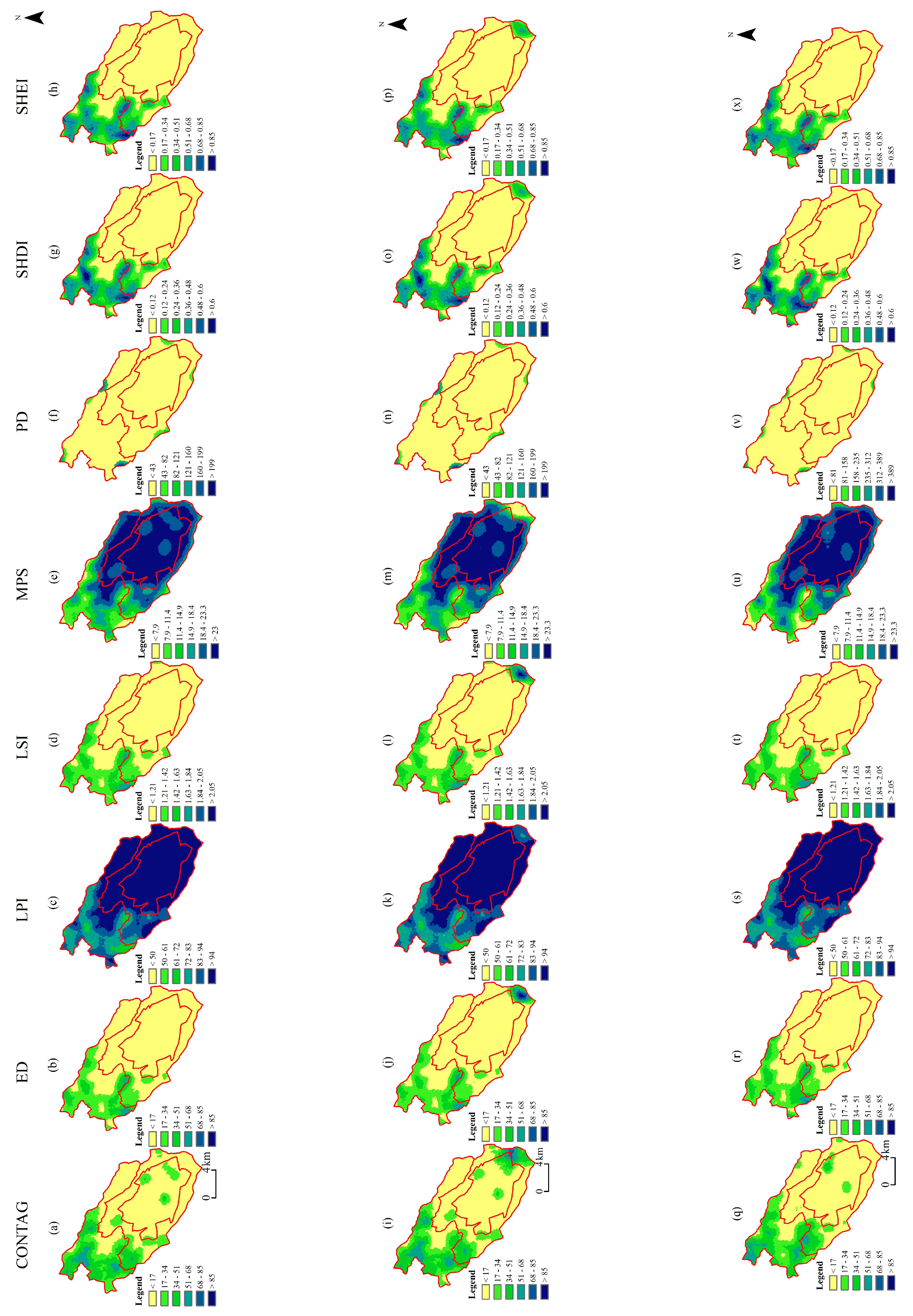
The landscape-level landscape pattern indexes for both NNRs are visualized in Figure 5 and Figure 6. Figure 5 reveals that the CONTAG and MPS indexes in ZlNNR exhibit a noticeable increasing trend, whereas the other indexes show no significant changes. The gap between the experimental zone and the core zone is prominent, with the extreme values of each landscape index observed in these areas. For instance, the ED and LSI of the core zone are lower, whereas the LPI is larger. Additionally, the PDs of the core zone and experimental zone are both lower, suggesting that the closer to the edge of ZlNNR, the higher the fragmentation of the landscape. However, SHDI and SHEI follow the pattern of experimental zone > buffer zone > core zone, indicating greater landscape diversity in the experimental zone. Figure 6 shows that the indexes inside MdfNNR have changed significantly in the southeast, displaying an increasing trend from 2000 to 2010 and a decreasing trend from 2010 to 2020. Among them, CONTAG, ED, LSI, SHDI, and SHEI all exhibit a pattern of experimental zone > buffer zone > core zone, whereas LPI and MPS follow the pattern of core zone > buffer zone > experimental zone. This suggests greater landscape diversity in the experimental zone and a less fragmented and more regular landscape in the core zone. Comparing the landscape indexes of the two NNRs reveals that MdfNNR experiences greater landscape fragmentation, whereas ZlNNR exhibits a more regular landscape shape.

3.3. NDVI

3.3.1. The Temporal Variation Characteristics

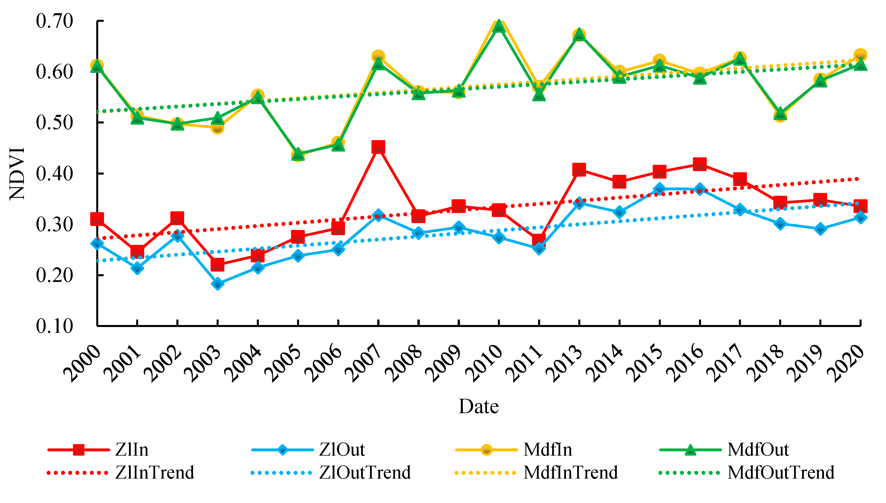
The interannual variation of the NDVI, as depicted in Figure 7, demonstrates that the annual average NDVI for each study area oscillated within a specific range and exhibited consistent temporal trends. The average annual NDVI inside and outside MdfNNR and ZlNNR ranged from 0.436–0.712, 0.439–0.690, 0.221–0.452, and 0.183–0.370, respectively. The annual average NDVI has been higher inside ZlNNR than outside over a period of nineteen years. The difference in NDVI between the inside and outside of MdfNNR is relatively small, but, overall, the inside has slightly higher NDVI values. The annual average NDVI of the MdfNNR was higher than that of the ZlNNR, primarily due to the predominance of forest land inside the MdfNNR. More specifically, the annual average NDVI of the MdfNNR experienced a steady decline from 2000 to 2003, although the rate of decline diminished each year. In 2010, the MdfNNR’s annual average NDVI peaked. From 2018 to 2020, the annual average NDVI of the MdfNNR consistently increased, with a more rapid increase observed inside than outside MdfNNR. The annual average NDVI of the ZlNNR consistently increased from 2003 to 2007, with a more rapid increase observed inside than outside ZlNNR. In 2007, the ZlNNR’s annual average NDVI reached its peak. Overall, both NNRs exhibited an upward trend in their annual average NDVI.

3.3.2. The Spatial Variation Characteristics

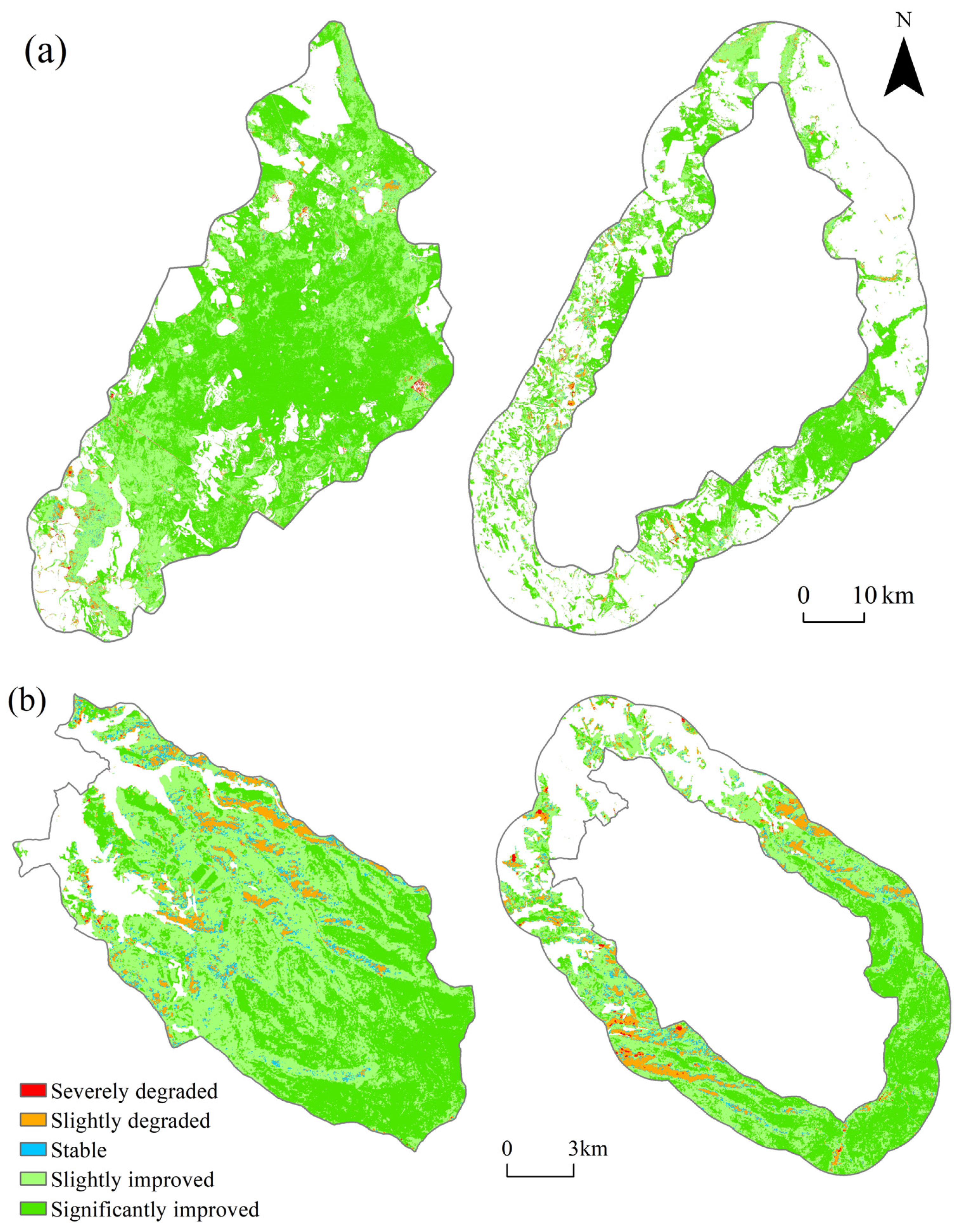
The distribution of improved, stable, and degraded vegetation inside ZlNNR accounted for 96.93%, 1.11%, and 1.96%, respectively (Table 9). In contrast, outside ZlNNR, they are 93.31%, 2.10%, and 4.59%. The vegetation improvement area was 3.62% greater inside than outside, and the vegetation degradation area was 2.63% less inside than outside. As shown in Figure 8a, the area of vegetation improvement in the ZlNNR was far greater than the area of vegetation degradation inside and outside. The areas with improved vegetation were predominantly located in the central region of the NNR and the southeast outside the NNR. Areas with slight vegetation improvement were predominantly distributed in the northeast and southwest regions of the NNR and various regions outside the NNR. Areas with stable vegetation were mainly found in the southwest region. In contrast, areas with slight and significant vegetation degradation were primarily located near water bodies and impervious lands.
The areas with improved vegetation, stable vegetation, and degraded vegetation in MdfNNR account for 88.35%, 4.84%, and 6.82%, respectively (Table 9). Conversely, outside MdfNNR, they are 82.96%, 5.55%, and 11.49%. The improved vegetation area was 5.39% greater inside than outside, and the degraded vegetation area was 4.68% less inside than outside. As shown in Figure 8b, the area of vegetation improvement was far greater than the area of vegetation degradation, whether inside MdfNNR or outside. Areas of notable vegetation improvement were predominantly situated in the southwest, whereas areas of slight improvement and stable vegetation were more dispersed. Regions with minor vegetation degradation were primarily found near roads, and areas with severe vegetation degradation were chiefly located near impervious land.
The time series analysis comparing the two PAs shows that ZlNNR has a higher percentage of areas with improving NDVI trends than MdfNNR. Specifically, the percentage is 8.59% higher in ZlNNR. For significantly improving trends, ZlNNR has 24.46% more area than MdfNNR. For slightly improving trends, ZlNNR has 15.88% less area than MdfNNR. On the other hand, the percentage of areas with degrading NDVI trends is 4.86% lower in ZlNNR than in MdfNNR. For severely degrading trends, ZlNNR has 0.06% more area than MdfNNR. For slightly degrading trends, ZlNNR has 6.96% less area than MdfNNR. However, the percentage of areas with stable NDVI is 3.45% lower in ZlNNR than in MdfNNR, indicating relatively stable NDVI in MdfNNR. In summary, the overall NDVI condition is better in ZlNNR compared to MdfNNR.

3.4. Comprehensive Analysis of Conservation Effectiveness

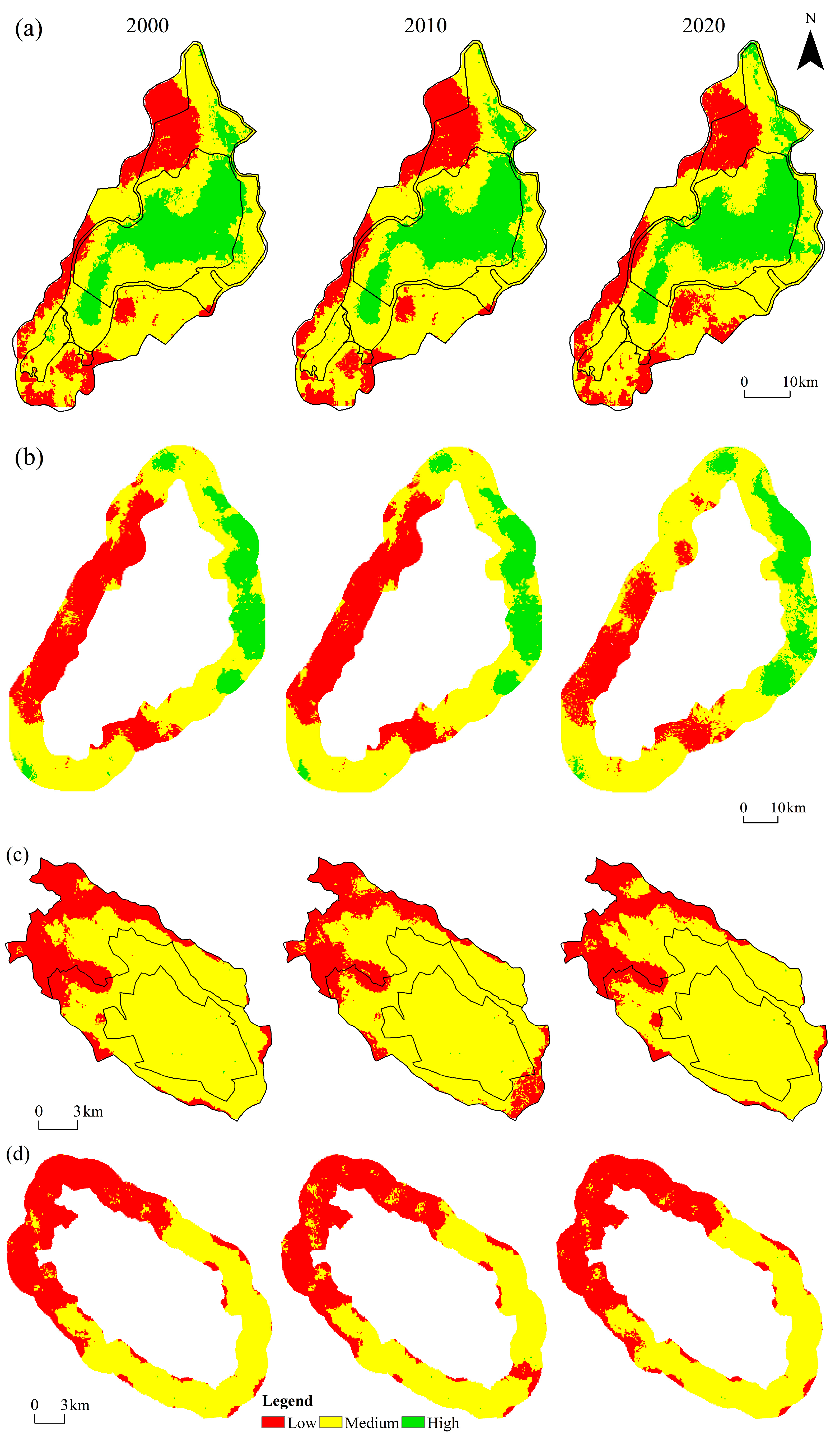
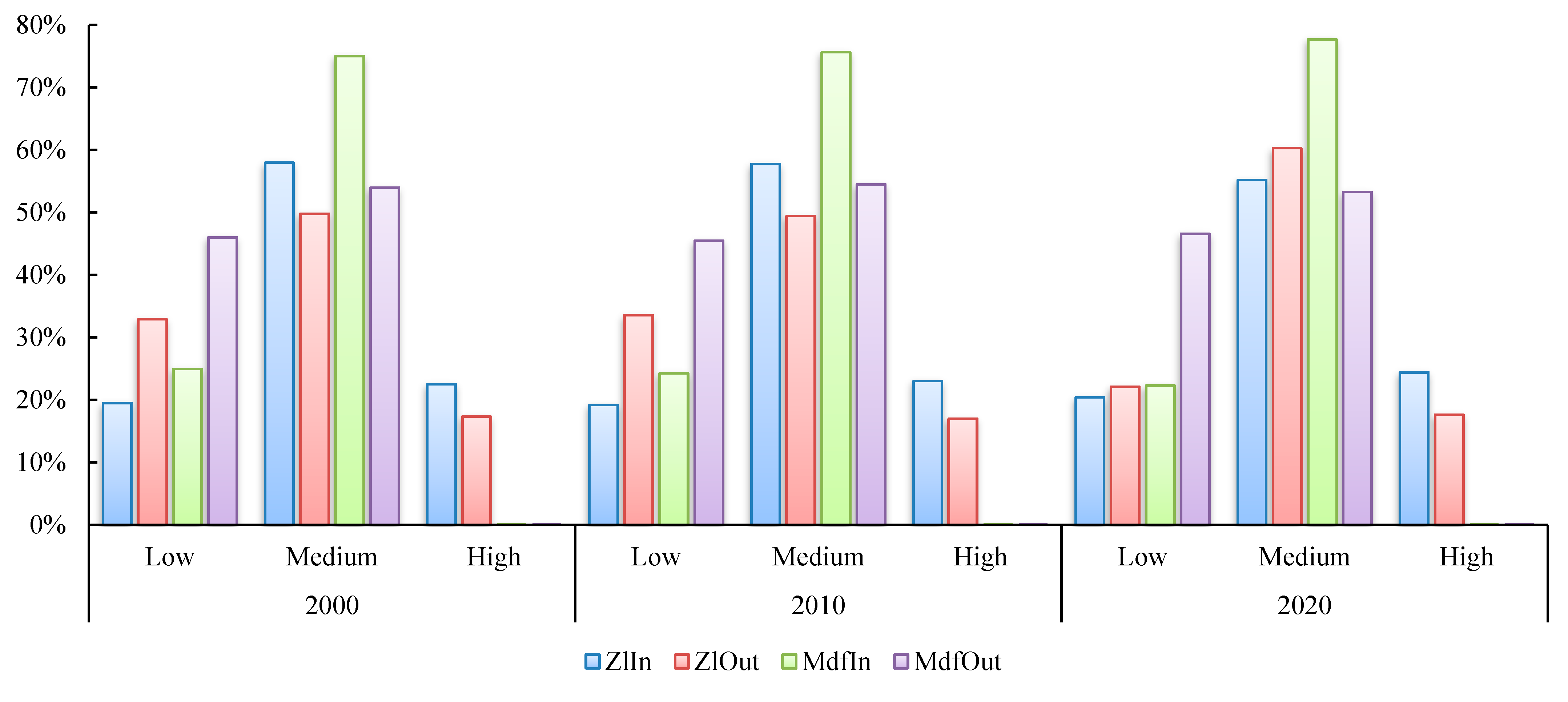
The weights assigned to each indicator in the study area were determined using the coefficient of variation method, as detailed in Table 10. Figure 9 presents the calculated results of conservation effectiveness for each study area. The proportions of the area corresponding to the three levels of conservation effectiveness in each study area were also computed, as depicted in Figure 10.
For inside ZlNNR, the area characterized by HE gradually increased, whereas the area of ME progressively decreased. The area of LE initially shrank and then increased. The relative proportions of the three conservation effectiveness levels in each period followed the pattern ME > HE > LE. Conversely, outside ZlNNR, the area of LE initially increased and then decreased, whereas the areas of both ME and HE first decreased and then increased. The relative proportions of the three conservation effectiveness levels in each period followed the pattern ME > LE > HE. Moreover, the inside had a higher area proportion of HE and ME than the outside each period, whereas LE was the opposite.
For inside MdfNNR, the area of LE continues to decrease, whereas the area of ME continues to increase, and the area of HE initially increased and then decreased. The relationship between the areas occupied by the three conservation effectiveness levels in each period was ME > LE > HE. Conversely, for outside MdfNNR, the area occupied by LE initially decreased and then increased, whereas the areas occupied by both ME and HE increased and then decreased. The relationship between the areas occupied by the three conservation effectiveness levels in each period was ME > HE > LE. LE areas inside MdfNNR were less than those outside each period, and the ME areas were higher than those outside each period. For HE areas, the difference between the inside and outside of the PAs was minimal.
Both ZlNNR and MdfNNR have served their purpose of protecting vegetation and landscape to a certain extent. As expected, the core zones offer the highest conservation effectiveness, followed by buffer and experimental zones. The areas of HE in ZlNNR were more significant than those in MdfNNR in each period, and the areas of ME and LE in ZlNNR were smaller than those in MdfNNR in each period. Therefore, the conservation effectiveness of ZlNNR was superior to that of MdfNNR.
4. Discussions

Our research contributes to the assessment of conservation effectiveness, to quantify the differences in conservation effectiveness across various types of PAs. We found that the conservation effectiveness of ZlNNR surpassed that of MdfNNR. This discrepancy could be attributed to a multitude of factors, including the size and location of the PAs, the level of economic development in the surrounding areas, and local population density. Future studies could delve deeper into these factors, providing valuable insights that could inform the creation of more effective conservation strategies and policies.

4.1. Analysis of Changes in Conservation Effectiveness and Their Driving Forces

Our research findings reveal that the degree of land use change in ZlNNR was relatively less than that observed in MdfNNR. This disparity can be attributed to the unique geographical locations and climatic characteristics of the two NNRs. ZlNNR, situated in a water-abundant environment, has limited human activity, and the implementation of green policies has further mitigated damage to wetlands. Consequently, changes in land use are primarily driven by climatic factors. Conversely, MdfNNR is an urbanized area with extensive transport networks and a high rate of economic growth. Here, societal and economic factors primarily shape land use transformations. Numerous studies have suggested that intense human intervention often leads to significant land degradation [21,71,84].
Our research indicates that MdfNNR experienced a higher degree of landscape fragmentation, largely due to its extensive transport infrastructure and dense network of roads [39]. This fragmentation of the internal landscape hinders species movement, thereby obstructing the effective preservation of biodiversity. Conversely, ZlNNR also saw a surge in road construction during the 1990s, primarily due to the development of highways and railways, which influenced landscape fragmentation [98,99]. However, the linear characteristics of highways and railways facilitate ecotourism growth and make it easier to mitigate their adverse impacts on the ecosystem. Moreover, ZlNNR’s diverse land use types and robust ecological features enhance its resilience to landscape fragmentation. Since the implementation of various protective measures in 2005 [61], the degree of landscape fragmentation in ZlNNR has significantly decreased, and the landscape diversity and connectivity have improved. This improvement can be attributed to the enhanced interconnectivity between the core area, buffer zone, and external environment, achieved through the construction and restoration of ecological corridors, the building of ecological bridges, and the implementation of slope greening measures. These initiatives have effectively mitigated the negative impacts of previous road construction, thereby establishing a solid foundation for the sustainable conservation of regional biodiversity.
Our NDVI study results indicate that the percentage of areas exhibiting an improving trend is higher for ZlNNR than for MdfNNR, whereas the percentage of areas exhibiting a degrading trend is lower for ZlNNR compared to MdfNNR. Overall, the NDVI conservation effectiveness of MdfNNR was inferior to that of ZlNNR. This slightly lower conservation performance of MdfNNR could be attributed to the greater impact of human activities and a prolonged drought from 1999 to 2002 [100,101]. Although ZlNNR also experienced this concurrent drought, a long-term water replenishment mechanism implemented since 2005 contributed to the earlier recovery of the NDVI [60,61].
The core area of NNRs typically serves a pivotal role in safeguarding biodiversity, ecosystems, and other related aspects [12]. This protective function facilitates the congregation and survival of various species, thereby enhancing the effectiveness of biodiversity and ecosystem conservation within the area. In our study, the core area, experiencing minimal external interference, presented a relatively stable and intact ecological environment, leading to a concentration of HE regions. The overall conservation effectiveness of ZlNNR surpassed that of MdfNNR, a finding that is consistent with our observations on land use, landscape patterns, and NDVI in the two NNRs. This superior performance can be attributed to ZlNNR’s robust natural attributes, more comprehensive ecological environment, and higher landscape connectivity. In contrast, MdfNNR faced significant ecological and environmental disturbances due to human activities, which inevitably curtailed its conservation effectiveness, leading to differential impacts between the two regions. To enhance the conservation effectiveness of MdfNNR, it is imperative to minimize the damage inflicted on its ecological environment by human activities [102]. The implementation of practical measures such as controlling unreasonable development and usage, restoring ecological corridors, and improving landscape connectivity could significantly bolster the ecological security and biodiversity conservation effectiveness of MdfNNR. Climate change, as a natural factor, can also exert substantial impacts on biodiversity and ecosystems in different regions [103]. For the effective and long-term protection of biodiversity in PAs, it is necessary to mitigate both the negative impacts of human activities and natural factors concurrently.
Holistic, multi-scale, and interconnected contemplation, strategizing, and management are important, yet still relatively lacking, aspects of current PA management [32]. The results of this study emphasize the necessity of adaptive management tailored to different ecosystem types. The studied wetland PA and forest PA require different management measures. Wetlands have higher sensitivity and require strict protection measures and proposing ecological restoration projects [33], while also needing more proactive restoration measures to improve degraded forests. Comparative results show management plans must consider the unique ecological characteristics, species compositions, and ecological functions of each ecosystem. The inherent complexities and incompatibilities between systems imply specialized PAs for particular ecosystems may allow more customized and effective protection. Establishing ecosystem PAs, safeguarding the unique attributes of habitats such as wetlands, forests, and grasslands, maintains their integrity. It enables tailored monitoring, restoration projects, and policy fine-tuning to local ecology. However, we still know little about future habitat suitability in PAs for colonization by alien species. Under climate change, predicting and assessing the receptivity of different ecosystems to alien organisms provides a basis for vulnerability assessments and adaptive strategy development. Additionally, concrete assessments of native species in PAs of varying ecosystems are needed to identify highly vulnerable species within different PA types, enabling timely targeted translocation [33]. Furthermore, our research found that both core and buffer zones of both PAs also experienced varying degrees of anthropogenic disturbance, although impacts were smaller in core zones. This illustrated that the core and buffer zones of different types of PAs had not been completely free from disturbance. In the future, the administration of PAs and higher-level departments will need to invest more manpower and material resources, increase patrol efforts, ensure the safety of protected objects, and achieve the purpose of on-site protection. Therefore, while establishing multifunctional PAs, developing specialized PAs based on specific ecosystems remains an important strategy for comprehensive and adaptive protection management.

4.2. Evaluation on Research Method Selection and Application

Land use serves as a significant indicator of the interaction between human activities and ecosystems [104], with extensive cropland areas serving as a stark testament to human influence. The transfer matrix of land use reveals the trends and principles of land use changes by examining the exchanges among various land use categories at different time points. The land use dynamic index is a comprehensive metric that encapsulates the direction, pace, and intensity of land use changes, offering superior practicality and advantages [70]. These two methods have been widely utilized in land use studies within PAs. Yan [71] and Mu [21] employed the land use dynamic index to monitor and evaluate the spatiotemporal changes of wetlands, revealing a lack of effectiveness in wetland conservation, a finding that contrasts with our results. Using a transition matrix from a different land use classification system, which subdivides forests into three categories, Bonilla observed increases in forest cover of 5% and 3% inside and outside PAs, respectively [105]. In contrast to previous research [73,105,106], we utilized the aforementioned two methods to conduct a comprehensive and accurate analysis of land use variation. In our study, forests both inside and outside the MdfNNR exhibited a decreasing trend. However, the declining trend inside the reserve was less pronounced than outside, which, to some extent, underscores the effectiveness of conservation efforts.
We used the GlobeLand30 data, which has emerged as a widely accepted resource for analyzing land use patterns [8,67], to investigate land use changes. In contrast, the previous research [61] conducted relied on the China Multi-temporal Land Use Remote Sensing Monitoring Dataset of the Resource and Environmental Science and Data Center, whereas other scholars opted for Landsat and Sentinel images for land use classification [107,108]. Though each of these data sources have their unique advantages, they vary in their estimations of the extent of different land use types, primarily due to differences in data quality and classification methods. Our investigation indicates that the degree of land use changes in ZlNNR was minimal between 2000 and 2010, with more noticeable variations emerging between 2010 and 2020. This sudden shift between these two periods differs from the findings of previous research [61,107,108]. This discrepancy is primarily due to inconsistencies in small-scale land use classification across different datasets. Therefore, we propose that future research should more effectively consider the scale and location of the study area when selecting data sources. This approach will enable a more accurate analysis of land use patterns.
In contrast to previous studies, the landscape index chosen for this research is distinguished by its comprehensive scope and systematic approach. Earlier studies, such as Mu [21], evaluated the conservation effectiveness of wetland conservation areas based solely on landscape fragmentation, whereas Lu [38] relied exclusively on the Landscape Development Intensity Index for their assessments. In this study, we utilized ten landscape indexes spanning five different aspects, including patch characteristics, patch shape, landscape characteristics, landscape shape, and landscape diversity. This approach allowed us to create a comprehensive quantitative characterization of spatial and shape characteristics across patches and landscapes. This methodology enabled us to accurately analyze the landscape patterns of PAs within a scientific and comprehensive framework. Moreover, we also adopted a visual analysis of landscape indexes, which offers superior analytical efficiency compared to previous studies [109,110,111,112], benefiting both researchers and readers. We deviated from the traditional moving window method [76,113] and instead embraced a combination of grid analysis and Kriging interpolation to provide accurate landscape boundary analyses. This approach aligns more closely with the latest trends in research.
The combination of the Theil–Sen median trend analysis and the Mann–Kendall test has proven to be a reliable approach for time series analysis. This method offers several advantages over univariate linear regression analysis, including the lack of requirement for data to follow a normal distribution, reduced sensitivity to outliers and extreme values, the effective detection of sequence trends and change points, and lower susceptibility to errors. Furthermore, this method is relatively straightforward to calculate, enhancing its practical applicability [84,114]. In their research on vegetation coverage in the Yellow River Basin, Jiang [84] also employed the Hurst index. We attempted to use this method as well, but found that the Hurst index is more suitable for studies involving large-scale research areas.
To provide a comprehensive and accurate assessment of ecological environment changes within the PA, this study utilized the NDVI as the primary remote sensing evaluation indicator. NDVI is recognized for its ability to quantitatively characterize the growth status and distribution changes of vegetation. Its widespread application in the scientific community also enhances the comparability and credibility of research results [34,45,84]. Though the Fraction of Vegetation Cover (FVC) and Remote Sensing Ecological Index (RSEI) were initially tested for their applicability in detecting ecological environment changes, NDVI proved to be more effective. This was due to its superior ability to filter out external environmental interference and accurately extract vegetation information. Conversely, FVC and RSEI were found to be more susceptible to significant errors caused by other environmental factors, making it difficult to extract useful data related to the research objectives. Consequently, NDVI was chosen as the sole remote sensing indicator to detect spatiotemporal changes in the ecological environment of the PA and evaluate the effectiveness of its protection. Our research findings indicated that a higher percentage of vegetation exhibited an improvement trend inside the PA than outside, suggesting that the PA has a certain degree of effectiveness. This conclusion aligns with previous studies, which demonstrated that nature reserves contribute to the improvement of sustainable and stable geographical spaces [34].
In addition, this study leveraged the GEE platform, which has gained prominence in the realm of remote sensing image processing, thanks to the rapid advancement of computer technology. The datasets within the platform require no preprocessing, thereby enhancing research efficiency [47,115]. Our study highlights the efficacy of remote sensing as a tool for evaluating the conservation effectiveness of PAs. Interestingly, the results derived from remote sensing were found to be almost identical to those obtained through traditional ground-based methods. This congruence underscores the validity and reliability of remote sensing as a method for conservation assessment. However, the advantage of remote sensing over ground-based methods lies in its timeliness and convenience. Remote sensing allows for real-time data collection and analysis, which can significantly enhance the effectiveness of conservation efforts. Furthermore, it provides a convenient and less intrusive means of monitoring PAs, reducing the need for physical intrusion that could potentially disrupt the ecosystems under protection.
In this study, we developed a generalizable framework for assessing the conservation effectiveness of PAs by evaluating three key factors: land use, landscape pattern, and NDVI. These three factors apply to various types of PAs and can be visualized to improve the clarity and intuitiveness of the analysis. The framework can effectively compare the conservation effectiveness of different types of PAs, such as forest and wetland types. We objectively determined the weight of each factor using the coefficient of variation method and constructed a conservation effectiveness assessment model using weighted summation, making the assessment results more scientific and convincing. This highly operable model provides a standardized analytical framework and assessment method for evaluating the conservation effectiveness of different types of PAs. The assessment model established in this study possesses expansive applicability for appraising conservation effectiveness in extant PAs of all typologies, and proffers references for prospective PA planning, hence possessing salient practical value.

4.3. Limitations and Future Trends

NDVI can become saturated in areas of high-density green biomass, making it challenging to detect changes in regions with 100% vegetation coverage. Additionally, NDVI may not accurately reflect critical vegetation characteristics during seasonal peaks [48,116,117]. Furthermore, within the ZlNNR, when wetlands transitioned to grasslands, the NDVI may exhibit an increasing trend, which is a false indication of effectiveness. This is a limitation of NDVI as a single assessing index. Nevertheless, we used a multi-factor collaborative framework to diminish or compensate for such deficiencies in this study. Other factors capturing changes in land use type and habitat fragmentation could reveal when apparent “improvements” in vegetation greenness may counter-intuitively signal deteriorating conditions in PAs. Our study underscores the importance of examining conservation outcomes through diverse lenses to obtain a comprehensive perspective. Therefore, in our future work, it will be necessary to corroborate the results obtained using NDVI with other data sources, such as high-resolution imagery and field survey data. To achieve more precise NDVI results and research conclusions, it is crucial to select appropriate observation periods to minimize the impact of seasonal changes in spectral signals on a temporal scale. High-resolution data can enhance the discernibility of various vegetation and ecological features within pixels at the spatial scale, partially compensating for the limitations of NDVI data in areas of high vegetation coverage. However, achieving high temporal and spatial resolutions simultaneously presents a challenge. Moreover, existing spectral indicators have limitations in accurately inverting vegetation feature parameters [117]. Therefore, we strongly recommend that future research employs advanced remote sensing methods, such as microwave remote sensing, to monitor and evaluate the vegetation dynamics in PAs more accurately and comprehensively.
Apart from the types of PAs analyzed in this study, there are other important ecosystems such as wildlife and grasslands that merit attention. However, our current conservation effectiveness evaluation system does not encompass all types of PAs, presenting a challenge for future research. We aim to direct future research efforts towards addressing this limitation. To develop a comprehensive conservation effectiveness evaluation system, it is necessary to conduct extensive and in-depth studies on methodologies, indicators, and management techniques. This endeavor requires not only building upon existing research findings, but also collaborating with experts from various fields to establish a more comprehensive and scientifically rigorous evaluation framework and research paradigm. We are committed to achieving these objectives to provide increasingly accurate, comprehensive, and advanced scientific support for PA management. Furthermore, it is crucial to pay close attention to minimizing the spillover effects of PAs [118,119,120], an issue that will be a key focus of our future research endeavors.

5. Conclusions

The quantitative evaluation model established in this study utilizes technologies including land use dynamic index, transition matrix, landscape pattern analysis, and NDVI time series to accurately measure changes in ecological quality and conservation effectiveness across PAs with varying ecosystems. By comparing reserves protecting different ecosystems, this research validates the methodological approach of using multiple quantitative techniques to comprehensively evaluate indicators of conservation effectiveness. The novel ecological and technological methodologies introduced establish a scientific system to assess conservation effectiveness. We found that significant disparities were observed in land use changes between the two PAs. ZlNNR experienced a substantial impact from wetland reduction, whereas MdfNNR was predominantly affected by forest reduction. The landscape patterns inside and outside PAs exhibited notable differences, characterized by higher internal landscape quality and reduced fragmentation. Both reserves exhibited smaller internal fluctuations in landscape pattern indexes compared to external fluctuations, indicating relative ecological stability. However, ZlNNR demonstrated higher landscape quality and stability compared to MdfNNR. Additionally, the percentage area of NDVI in ZlNNR exhibited a more pronounced increasing trend versus MdfNNR. Our evaluation method holds substantial theoretical and practical value, enriching the foundation and techniques for evaluating nature reserve efficacy and offering innovation for ecology and environmental management fields.

Author Contributions

J.Z. wrote the manuscript. C.J. conceived the idea and framework of the study. T.C. reviewed and provided critical feedback. H.S. and X.J. analyzed data. All authors contributed to the manuscript. All authors have read and agreed to the published version of the manuscript.

Funding

The work was supported by the Natural Science Foundation of Heilongjiang Province of China (Fund number: LH2020C032, funder: Heilongjiang Provincial Department of Science and Technology).

Data Availability Statement

The GlobeLand30 is available at http://globallandcover.com/ (accessed on 10 April 2023). The remote sensing image data are available at https://code.earthengine.google.com/ (accessed on 29 June 2023).

Acknowledgments

We appreciate the Institute of Remote Sensing and Digital Earth for providing the GlobeLand30 dataset, as well as the Google Earth Engine platform for offering remote sensing datasets and cloud computing services. We also thank the Natural Science Foundation of Heilongjiang Province of China (LH2020C032).

Conflicts of Interest

The authors declare no conflict of interest.

References

  1. Dudley, N. Guidelines for Applying Protected Area Management Categories; IUCN: Gland, Switzerland, 2008; Volume 3. [Google Scholar]
  2. Dureuil, M.; Boerder, K.; Burnett, K.A.; Froese, R.; Worm, B. Elevated Trawling Inside Protected Areas Undermines Conservation Outcomes in a Global Fishing Hotspot. Science 2018, 362, 1403–1407. [Google Scholar] [CrossRef] [PubMed]
  3. Feng, C.T.; Cao, M.; Liu, F.Z.; Zhou, Y.; Du, J.H.; Zhang, L.B.; Huang, W.J.; Luo, J.W.; Li, J.S.; Wang, W. Improving Protected Area Effectiveness through Consideration of Different Human Pressure Baselines. Conserv. Biol. 2022, 36, e13887. [Google Scholar] [CrossRef]
  4. Hoffmann, S.; Irl, S.D.H.; Beierkuhnlein, C. Predicted Climate Shifts within Terrestrial Protected Areas Worldwide. Nat. Commun. 2019, 10, 4787. [Google Scholar] [CrossRef] [PubMed]
  5. Pack, S.M.; Ferreira, M.N.; Krithivasan, R.; Murrow, J.; Bernard, E.; Mascia, M.B. Protected Area Downgrading, Downsizing, and Degazettement (PADDD) in the Amazon. Biol. Conserv. 2016, 197, 32–39. [Google Scholar] [CrossRef]
  6. Pringle, R.M. Upgrading Protected Areas to Conserve Wild Biodiversity. Nature 2017, 546, 91–99. [Google Scholar] [CrossRef]
  7. Schulze, K.; Knights, K.; Coad, L.; Geldmann, J.; Leverington, F.; Eassom, A.; Marr, M.; Butchart, S.H.M.; Hockings, M.; Burgess, N.D. An Assessment of Threats to Terrestrial Protected Areas. Conserv. Lett. 2018, 11, e12435. [Google Scholar] [CrossRef]
  8. Meng, Z.Q.; Dong, J.W.; Ellis, E.C.; Metternicht, G.; Qin, Y.W.; Song, X.P.; Löfqvist, S.; Garrett, R.D.; Jia, X.P.; Xiao, X.M. Post-2020 Biodiversity Framework Challenged by Cropland Expansion in Protected Areas. Nat. Sustain. 2023, 6, 758–768. [Google Scholar] [CrossRef]
  9. Kelboro, G.; Stellmacher, T. Contesting the National Park Theorem? Governance and Land Use in Nech Sar National Park, Ethiopia; ZEF Working Paper Series; ZFF: Bonn, Germany, 2012; p. 104. [Google Scholar]
  10. Tang, X.P.; Jiang, Y.F.; Liu, Z.L.; Chen, J.Z.; Liang, B.K.; Lin, C. Top-Level Design of the Natural Protected Area System in China. For. Resour. Manag. 2019, 1, 1–7. [Google Scholar] [CrossRef]
  11. Wang, W.; Feng, C.T.; Liu, F.Z.; Li, J.S. Biodiversity Conservation in China: A Review of Recent Studies and Practices. Environ. Sci. Ecotechnol. 2020, 2, 100025. [Google Scholar] [CrossRef]
  12. Zhuang, H.F.; Xia, W.C.; Zhang, C.; Yang, L.; Wanghe, K.Y.; Chen, J.Z.; Luan, X.F.; Wang, W. Functional Zoning of China’s Protected Area Needs to be Optimized for Protecting Giant Panda. Glob. Ecol. Conserv. 2021, 25, e01392. [Google Scholar] [CrossRef]
  13. Achiso, Z. Biodiversity and Human Livelihoods in Protected Areas: Worldwide Perspective—A Review. SSR Inst. Int. J. Life Sci 2020, 6, 2565–2578. [Google Scholar] [CrossRef]
  14. Barnes, M. Aichi Targets: Protect Biodiversity, Not Just Area. Nature 2015, 526, 195. [Google Scholar] [CrossRef] [PubMed]
  15. Le Saout, S.; Hoffmann, M.; Shi, Y.; Hughes, A.; Bernard, C.; Brooks, T.M.; Bertzky, B.; Butchart, S.H.; Stuart, S.N.; Badman, T.; et al. Conservation. Protected Areas and Effective Biodiversity Conservation. Science 2013, 342, 803–805. [Google Scholar] [CrossRef] [PubMed]
  16. Bai, X.Y.; Du, P.J.; Guo, S.C.; Zhang, P.; Lin, C.; Tang, P.F.; Zhang, C. Monitoring Land Cover Change and Disturbance of the Mount Wutai World Cultural Landscape Heritage Protected Area, Based on Remote Sensing Time-Series Images from 1987 to 2018. Remote Sens. 2019, 11, 1332. [Google Scholar] [CrossRef]
  17. Scharsich, V.; Mtata, K.; Hauhs, M.; Lange, H.; Bogner, C. Analysing Land Cover and Land Use Change in the Matobo National Park and Surroundings in Zimbabwe. Remote Sens. Environ. 2017, 194, 278–286. [Google Scholar] [CrossRef]
  18. Wade, C.M.; Austin, K.G.; Cajka, J.; Lapidus, D.; Everett, K.H.; Galperin, D.; Maynard, R.; Sobel, A. What Is Threatening Forests in Protected Areas? A Global Assessment of Deforestation in Protected Areas, 2001–2018. Forests 2020, 11, 539. [Google Scholar] [CrossRef]
  19. Guo, Z.L.; Zhang, M.Y. The Conservation Efficacy of Coastal Wetlands in China Based on Landscape Development and Stress. Ocean Coast. Manag. 2019, 175, 70–78. [Google Scholar] [CrossRef]
  20. Bazelet, C.S.; Thompson, A.C.; Naskrecki, P. Testing the Efficacy of Global Biodiversity Hotspots for Insect Conservation: The Case of South African Katydids. PLoS ONE 2016, 11, e0160630. [Google Scholar] [CrossRef]
  21. Mu, Y.L.; Li, X.W.; Liang, C.; Li, P.; Guo, Y.; Liang, F.Y.; Bai, J.H.; Cui, B.S.; Bilal, H. Rapid Landscape Assessment for Conservation Effectiveness of Wetland National Nature Reserves across the Chinese Mainland. Glob. Ecol. Conserv. 2021, 31, e01842. [Google Scholar] [CrossRef]
  22. Simaika, J.P.; Samways, M.J. An Easy-to-Use Index of Ecological Integrity for Prioritizing Freshwater Sites and for Assessing Habitat Quality. Biodivers. Conserv. 2009, 18, 1171–1185. [Google Scholar] [CrossRef]
  23. Brown, C.J.; Bode, M.; Venter, O.; Barnes, M.D.; McGowan, J.; Runge, C.A.; Watson, J.E.; Possingham, H.P. Effective Conservation Requires Clear Objectives and Prioritizing Actions, Not Places or Species. Proc. Nat. Acad. Sci. USA 2015, 112, E4342. [Google Scholar] [CrossRef]
  24. Jenkins, C.N.; Van Houtan, K.S.; Pimm, S.L.; Sexton, J.O. US Protected Lands Mismatch Biodiversity Priorities. Proc. Nat. Acad. Sci. USA 2015, 112, 5081–5086. [Google Scholar] [CrossRef] [PubMed]
  25. Jia, M.M.; Wang, Z.M.; Zhang, Y.Z.; Mao, D.H.; Wang, C. Monitoring Loss and Recovery of Mangrove Forests During 42 Years: The Achievements of Mangrove Conservation in China. Int. J. Appl. Earth Obs. Geoinf. 2018, 73, 535–545. [Google Scholar] [CrossRef]
  26. Lu, C.Y.; Liu, J.F.; Jia, M.M.; Liu, M.Y.; Man, W.D.; Fu, W.W.; Zhong, L.X.; Lin, X.Q.; Su, Y.; Gao, Y.B. Dynamic Analysis of Mangrove Forests Based on an Optimal Segmentation Scale Model and Multi-Seasonal Images in Quanzhou Bay, China. Remote Sens. 2018, 10, 2020. [Google Scholar] [CrossRef]
  27. Burke, M.; Driscoll, A.; Lobell, D.B.; Ermon, S. Using satellite imagery to understand and promote sustainable development. Science 2021, 371, eabe8628. [Google Scholar] [CrossRef]
  28. Garg, J.K. Wetland Assessment, Monitoring and Management in India Using Geospatial Techniques. J. Environ. Manag. 2015, 148, 112–123. [Google Scholar] [CrossRef] [PubMed]
  29. Powlen, K.A.; Gavin, M.C.; Jones, K.W. Management effectiveness positively influences forest conservation outcomes in protected areas. Biol. Conserv. 2021, 260, 109192. [Google Scholar] [CrossRef]
  30. Zhu, P.; Huang, L.; Xiao, T.; Wang, J.B. Dynamic Changes of Habitats in China’s Typical National Nature Reserves on Spatial and Temporal Scales. J. Geogr. Sci. 2018, 28, 778–790. [Google Scholar] [CrossRef]
  31. Krajewski, P. Monitoring of landscape transformations within landscape parks in Poland in the 21st century. Sustainability 2019, 11, 2410. [Google Scholar] [CrossRef]
  32. Gatiso, T.T.; Kulik, L.; Bachmann, M.; Bonn, A.; Bösch, L.; Eirdosh, D.; Freytag, A.; Hanisch, S.; Heurich, M.; Sop, T. Effectiveness of protected areas influenced by socio-economic context. Nat. Sustain. 2022, 5, 861–868. [Google Scholar] [CrossRef]
  33. Xin, Y.; Yang, Z.; Du, Y.; Cui, R.; Xi, Y.; Liu, X. Vulnerability of protected areas to future climate change, land use modification, and biological invasions in China. Ecol. Appl. 2023, e2831, early view. [Google Scholar] [CrossRef] [PubMed]
  34. Zhao, S.Q.; Zhao, X.; Zhao, J.C.; Liu, N.J.; Sun, M.M.; Mu, B.H.; Sun, N.; Guo, Y.K. Grassland Conservation Effectiveness of National Nature Reserves in Northern China. Remote Sens. 2022, 14, 1760. [Google Scholar] [CrossRef]
  35. Lawler, J.J.; Lewis, D.J.; Nelson, E.; Plantinga, A.J.; Polasky, S.; Withey, J.C.; Helmers, D.P.; Martinuzzi, S.; Pennington, D.; Radeloff, V.C. Projected Land-Use Change Impacts on Ecosystem Services in the United States. Proc. Nat. Acad. Sci. USA 2014, 111, 7492–7497. [Google Scholar] [CrossRef] [PubMed]
  36. Ning, J.; Liu, J.Y.; Kuang, W.H.; Xu, X.L.; Zhang, S.W.; Yan, C.Z.; Li, R.D.; Wu, S.X.; Hu, Y.F.; Du, G.M. Spatiotemporal Patterns and Characteristics of Land-Use Change in China During 2010–2015. J. Geogr. Sci. 2018, 28, 547–562. [Google Scholar] [CrossRef]
  37. Mooney, H.A.; Duraiappah, A.; Larigauderie, A. Evolution of Natural and Social Science Interactions in Global Change Research Programs. Proc. Nat. Acad. Sci. USA 2013, 110, 3665–3672. [Google Scholar] [CrossRef]
  38. Lu, C.Y.; Wang, Z.M.; Li, L.; Wu, P.Z.; Mao, D.H.; Jia, M.M.; Dong, Z.Y. Assessing the Conservation Effectiveness of Wetland Protected Areas in Northeast China. Wetl. Ecol. Manag. 2016, 24, 381–398. [Google Scholar] [CrossRef]
  39. Hu, J.Y.; Zhang, J.X.; Li, Y.Q. Exploring the Spatial and Temporal Driving Mechanisms of Landscape Patterns on Habitat Quality in a City Undergoing Rapid Urbanization Based on GTWR and MGWR: The Case of Nanjing, China. Ecol. Indic. 2022, 143, 109333. [Google Scholar] [CrossRef]
  40. Meyer, S.R.; Beard, K.; Cronan, C.S.; Lilieholm, R.J. An Analysis of Spatio-Temporal Landscape Patterns for Protected Areas in Northern New England: 1900–2010. Landsc. Ecol. 2015, 30, 1291–1305. [Google Scholar] [CrossRef]
  41. Sowińska-Świerkosz, B.N.; Soszyński, D. Landscape Structure versus the Effectiveness of Nature Conservation: Roztocze Region Case Study (Poland). Ecol. Indic. 2014, 43, 143–153. [Google Scholar] [CrossRef]
  42. Vorovencii, I. Quantifying Landscape Pattern and Assessing the Land Cover Changes in Piatra Craiului National Park and Bucegi Natural Park, Romania, Using Satellite Imagery and Landscape Metrics. Environ. Monit. Assess. 2015, 187, 692. [Google Scholar] [CrossRef]
  43. Eckert, S.; Hüsler, F.; Liniger, H.; Hodel, E. Trend Analysis of MODIS NDVI Time Series for Detecting Land Degradation and Regeneration in Mongolia. J. Arid. Environ. 2015, 113, 16–28. [Google Scholar] [CrossRef]
  44. Hausner, M.B.; Huntington, J.L.; Nash, C.; Morton, C.; McEvoy, D.J.; Pilliod, D.S.; Hegewisch, K.C.; Daudert, B.; Abatzoglou, J.T.; Grant, G. Assessing the Effectiveness of Riparian Restoration Projects Using Landsat and Precipitation Data from the Cloud-Computing Application ClimateEngine. org. Ecol. Eng. 2018, 120, 432–440. [Google Scholar] [CrossRef]
  45. Wu, Z.T.; Wu, J.J.; He, B.; Liu, J.H.; Wang, Q.F.; Zhang, H.; Liu, Y. Drought Offset Ecological Restoration Program-Induced Increase in Vegetation Activity in the Beijing-Tianjin Sand Source Region, China. Environ. Sci. Technol. 2014, 48, 12108–12117. [Google Scholar] [CrossRef] [PubMed]
  46. Wang, Y.; Zhao, Y.H.; Wu, J.S. Dynamic Monitoring of Long Time Series of Ecological Quality in Urban Agglomerations Using Google Earth Engine Cloud Computing: A Case Study of the Guangdong-Hong Kong-Macao Greater Bay Area, China. Acta Ecol. Sin. 2020, 40, 8461–8473. [Google Scholar] [CrossRef]
  47. Xiong, Y.; Xu, W.H.; Lu, N.; Huang, S.D.; Wu, C.; Wang, L.G.; Dai, F.; Kou, W.L. Assessment of Spatial-Temporal Changes of Ecological Environment Quality Based on RSEI and GEE: A Case Study in Erhai Lake Basin, Yunnan Province, China. Ecol. Indic. 2021, 125, 107518. [Google Scholar] [CrossRef]
  48. Wang, Z.; Wei, C.Y.; Liu, X.N.; Zhu, L.H.; Yang, Q.; Wang, Q.Y.; Zhang, Q.; Meng, Y.Y. Object-Based Change Detection for Vegetation Disturbance and Recovery Using Landsat Time Series. GISci. Remote Sens. 2022, 59, 1706–1721. [Google Scholar] [CrossRef]
  49. Marshall, A.R.; Willcock, S.; Platts, P.J.; Lovett, J.C.; Balmford, A.; Burgess, N.D.; Latham, J.E.; Munishi, P.K.T.; Salter, R.; Shirima, D.D. Measuring and modelling above-ground carbon and tree allometry along a tropical elevation gradient. Biol. Conserv. 2012, 154, 20–33. [Google Scholar] [CrossRef]
  50. Taubert, F.; Fischer, R.; Groeneveld, J.; Lehmann, S.; Muller, M.S.; Rodig, E.; Wiegand, T.; Huth, A. Global Patterns of Tropical Forest Fragmentation. Nature 2018, 554, 519–522. [Google Scholar] [CrossRef]
  51. Zhao, H.W.; Wu, R.D.; Long, Y.C.; Hu, J.M.; Yang, F.L.; Jin, T.; Wang, J.J.; Hu, P.J.; Wu, W.; Diao, Y.X. Individual-Level Performance of Nature Reserves in Forest Protection and the Effects of Management Level and Establishment Age. Biol. Conserv. 2019, 233, 23–30. [Google Scholar] [CrossRef]
  52. Li, X.J.; Du, H.Q.; Mao, F.J.; Zhou, G.M.; Han, N.; Xu, X.J.; Liu, Y.L.; Zheng, J.L.; Dong, L.F.; Zhang, M. Assimilating Spatiotemporal MODIS LAI Data with a Particle Filter Algorithm for Improving Carbon Cycle Simulations for Bamboo Forest Ecosystems. Sci. Total Environ. 2019, 694, 133803. [Google Scholar] [CrossRef]
  53. Wu, Y.F.; Zhang, G.X. Review of Development, Frontiers and Prospects of Wetlands Eco-Hydrological Models. Acta Ecol. Sin. 2018, 38, 2588–2598. [Google Scholar] [CrossRef]
  54. Asselen, S.V.; Verburg, P.H.; Vermaat, J.E.; Janse, J.H. Drivers of Wetland Conversion: A Global Meta-Analysis. PLoS ONE 2013, 8, e81292. [Google Scholar] [CrossRef] [PubMed]
  55. Xiao, Y.; Zhang, L.; Zhang, L.Y.; Xiao, Y.; Zheng, H.; OuYang, Z.Y. Spatial Variation Analysis of Biodiversity in the Bohai Region Coastal Wetland. Acta Ecol. Sin. 2018, 38, 909–916. [Google Scholar] [CrossRef]
  56. Mahdianpari, M.; Jafarzadeh, H.; Granger, J.E.; Mohammadimanesh, F.; Brisco, B.; Salehi, B.; Homayouni, S.; Weng, Q.H. A Large-Scale Change Monitoring of Wetlands Using Time Series Landsat Imagery on Google Earth Engine: A Case Study in Newfoundland. Gisci. Remote Sens. 2020, 57, 1102–1124. [Google Scholar] [CrossRef]
  57. Shang, H.M.; Xi, M.; Li, Y.; Kong, F.L.; Wang, S. Evaluation of Changes in the Ecosystem Services of Jiaozhou Bay Coastal Wetland. Acta Ecol. Sin. 2018, 38, 421–431. [Google Scholar] [CrossRef]
  58. Montesino Pouzols, F.; Toivonen, T.; Di Minin, E.; Kukkala, A.S.; Kullberg, P.; Kuusterä, J.; Lehtomäki, J.; Tenkanen, H.; Verburg, P.H.; Moilanen, A. Global Protected Area Expansion Is Compromised by Projected Land-Use and Parochialism. Nature 2014, 516, 383–386. [Google Scholar] [CrossRef] [PubMed]
  59. Feng, X.; Zhang, G.; Jun Xu, Y. Simulation of hydrological processes in the Zhalong wetland within a river basin, Northeast China. Hydrol. Earth. Syst. Sci. 2013, 17, 2797–2807. [Google Scholar] [CrossRef]
  60. Chen, L.W.; Liu, S.X.; Wu, Y.F.; Xu, Y.J.; Chen, S.B.; Pang, S.L.; Gao, Z.T.; Zhang, G.X. Does ecological water replenishment help prevent a large wetland from further deterioration? Results from the zhalong nature reserve, China. Remote Sens. 2020, 12, 3449. [Google Scholar] [CrossRef]
  61. Yang, Y.Q.; Gong, A.D.; Zhang, Y.H.; Chen, Y.L. Dynamic Changes in Zhalong Wetland Landscape from 1980 to 2015. J. Beijing Norm. Univ. 2021, 57, 624–630. [Google Scholar] [CrossRef]
  62. Na, X.; Zang, S.; Wu, C.; Tian, Y.; Li, W. Hydrological regime monitoring and mapping of the Zhalong wetland through integrating time series Radarsat-2 and Landsat imagery. Remote Sens. 2018, 10, 702. [Google Scholar] [CrossRef]
  63. Gao, Z.F.; Deng, L.B.; Chen, D.L. Ecological evaluation of Mudanfeng National Nature Reserve in Heilongjiang Province. J. Cent. South Univ. 2012, 32, 106–109. [Google Scholar] [CrossRef]
  64. Yang, M.; Cai, T.; Ju, C.; Zou, H. Evaluating spatial structure of a mixed broad-leaved/Korean pine forest based on neighborhood relationships in Mudanfeng National Nature Reserve, China. J. For. Res. 2019, 30, 1375–1381. [Google Scholar] [CrossRef]
  65. Brovelli, M.A.; Molinari, M.E.; Hussein, E.; Chen, J.; Li, R. The First Comprehensive Accuracy Assessment of GlobeLand30 at a National Level: Methodology and Results. Remote Sens. 2015, 7, 4191–4212. [Google Scholar] [CrossRef]
  66. Long, L.; Chen, Y.Y.; Song, S.J.; Zhang, X.L.; Jia, X.; Lu, Y.G.; Liu, G. Remote Sensing Monitoring of Pine Wilt Disease Based on Time-Series Remote Sensing Index. Remote Sens. 2023, 15, 360. [Google Scholar] [CrossRef]
  67. Jun, C.; Ban, Y.F.; Li, S.N. Open Access to Earth Land-Cover Map. Nature 2014, 514, 434. [Google Scholar] [CrossRef]
  68. Sun, C.; Li, J.; Liu, Y.; Cao, L.; Zheng, J.; Yang, Z.; Ye, J.; Li, Y. Ecological quality assessment and monitoring using a time-series remote sensing-based ecological index (ts-RSEI). Gisci. Remote Sens. 2022, 59, 1793–1816. [Google Scholar] [CrossRef]
  69. Gorelick, N.; Hancher, M.; Dixon, M.; Ilyushchenko, S.; Thau, D.; Moore, R. Google Earth Engine: Planetary-scale geospatial analysis for everyone. Remote Sens. Environ. 2017, 202, 18–27. [Google Scholar] [CrossRef]
  70. Zhu, H.Y.; Li, X.B. Discussion on the Index Method of Regional Land Use Change. Acta Geogr. Sin. 2003, 58, 643–650. [Google Scholar] [CrossRef]
  71. Yan, F.Q.; Zhang, S.W.; Liu, X.T.; Yu, L.X.; Chen, D.; Yang, J.C.; Yang, C.B.; Bu, K.; Chang, L.P. Monitoring spatiotemporal changes of marshes in the Sanjiang Plain, China. Ecol. Eng. 2017, 104, 184–194. [Google Scholar] [CrossRef]
  72. Zhang, M.M.; Zhang, L.J.; Li, H.J.; Cai, J.Y.; Hu, C.S. Study on the Landscape Pattern Changes and the Landscape Development Intensity of Caohai National Nature Reserve, Guizhou. J. Ecol. Rural. Environ. 2019, 35, 300–306. [Google Scholar] [CrossRef]
  73. Deng, S.Y. Study on the Effectiveness Evaluation of Protection of Minjiang Estuary Wetland. Master’s Thesis, Fujian Agriculture and Forestry University, Fuzhou, China, 2020. [Google Scholar]
  74. Guo, Z.L.; Zhang, M.Y.; Liu, W.W.; Liu, Z.J.; Zhang, Y.G. Landscape Pattern and Conservation Efficacy Analysis of Hengshui Lake National Nature Reserve, Hebei during Three Periods. Wetl. Sci. 2021, 19, 170–177. [Google Scholar] [CrossRef]
  75. Liu, C.Y.; Zhang, K.; Liu, J.P. A Long-Term Site Study for the Ecological Risk Migration of Landscapes and Its Driving Forces in the Sanjiang Plain from 1976 to 2013. Acta Ecol. Sin. 2018, 38, 3729–3740. [Google Scholar] [CrossRef]
  76. Lü, L.T.; Zhang, J.; Peng, Q.Z.; Ren, F.P.; Jiang, Y. Landscape Pattern Analysis and Prediction in the Dongjiang River Basin. Acta Ecol. Sin. 2019, 39, 6850–6859. [Google Scholar] [CrossRef]
  77. Zhu, C.M.; Zhang, X.L.; Zhou, M.M.; He, S.; Gan, M.Y.; Yang, L.X.; Wang, K. Impacts of Urbanization and Landscape Pattern on Habitat Quality Using OLS and GWR Models in Hangzhou, China. Ecol. Indic. 2020, 117, 106654. [Google Scholar] [CrossRef]
  78. Zhou, J.J.; Luo, C.Y.; Ma, D.F.; Shi, W.; Wang, L.Y.; Guo, Z.N.; Tang, H.T.; Wang, X.; Wang, J.R.; Liu, C.F. The Impact of Land Use Landscape Pattern on River Hydrochemistry at Multi-Scale in an Inland River Basin, China. Ecol. Indic. 2022, 143, 109334. [Google Scholar] [CrossRef]
  79. Cui, L.J.; Li, W.; Zhang, M.Y.; Wang, Y.F. Changes in Landscape Pattern of Mangrove Wetlands and Their Driving Force in the Luoyang River Estuary, Fujian Province. J. Beijing For. Univ. 2010, 32, 106–112. [Google Scholar] [CrossRef]
  80. Townsend, C.R.; Dolédec, S.; Norris, R.; Peacock, K.; Arbuckle, C. The Influence of Scale and Geography on Relationships between Stream Community Composition and Landscape Variables: Description and Prediction. Freshw. Biol. 2003, 48, 768–785. [Google Scholar] [CrossRef]
  81. Shannon, C.E. A Mathematical Theory of Communication. ACM Sigmobile Mob. Comput. Commun. Rev. 2001, 5, 3–55. [Google Scholar] [CrossRef]
  82. Goward, S.N.; Xue, Y.K.; Czajkowski, K.P. Evaluating land surface moisture conditions from the remotely sensed temperature/vegetation index measurements: An exploration with the simplified simple biosphere model. Remote Sens. Environ. 2002, 79, 225–242. [Google Scholar] [CrossRef]
  83. Meng, Y.Y.; Hou, B.; Ding, C.; Huang, L.; Guo, Y.P.; Tang, Z.Y. Spatiotemporal patterns of planted forests on the Loess Plateau between 1986 and 2021 based on Landsat NDVI time-series analysis. Gisci. Remote Sens. 2023, 60, 2185980. [Google Scholar] [CrossRef]
  84. Jiang, W.G.; Yuan, L.H.; Wang, W.J.; Cao, R.; Zhang, Y.F.; Shen, W.M. Spatio-Temporal Analysis of Vegetation Variation in the Yellow River Basin. Ecol. Indic. 2015, 51, 117–126. [Google Scholar] [CrossRef]
  85. Sun, L. Dynamic monitoring and driving factor analysis of vegetation change in Sichuan province. Southwest China J. Agric. Sci. 2023, 36, 1082–1089. [Google Scholar] [CrossRef]
  86. Sen, P.K. Estimates of the Regression Coefficient Based on Kendall's Tau. J. Am. Stat. Assoc. 1968, 63, 1379–1389. [Google Scholar] [CrossRef]
  87. Theil, H. A Rank-Invariant Method of Linear and Polynomial Regression Analysis. Proc. K. Ned. Akad. Wet. 1950, 53, 386–392, 521–525, 1397–1412. [Google Scholar]
  88. Kendall, M.G. Rank Correlation Methods; Griffin: London, UK, 1975. [Google Scholar]
  89. Tošić, I. Spatial and Temporal Variability of Winter and Summer Precipitation over Serbia and Montenegro. Theor. Appl. Climatol. 2004, 77, 47–56. [Google Scholar] [CrossRef]
  90. Fensholt, R.; Langanke, T.; Rasmussen, K.; Reenberg, A.; Prince, S.D.; Tucker, C.; Scholes, R.J.; Le, Q.B.; Bondeau, A.; Eastman, R. Greenness in Semi-Arid Areas Across the Globe 1981–2007—An Earth Observing Satellite Based Analysis of Trends and Drivers. Remote Sens. Environ. 2012, 121, 144–158. [Google Scholar] [CrossRef]
  91. Fensholt, R.; Proud, S.R. Evaluation of Earth Observation Based Global Long Term Vegetation Trends—Comparing GIMMS and MODIS Global NDVI Time Series. Remote Sens. Environ. 2012, 119, 131–147. [Google Scholar] [CrossRef]
  92. Lunetta, R.S.; Knight, J.F.; Ediriwickrema, J.; Lyon, J.G.; Worthy, L.D. Land-Cover Change Detection Using Multi-Temporal MODIS NDVI Data. Remote Sens. Environ. 2006, 105, 142–154. [Google Scholar] [CrossRef]
  93. Milich, L.; Weiss, E. GAC NDVI Interannual Coefficient of Variation (CoV) Images: Ground Truth Sampling of the Sahel along North-South Transects. Int. J. Remote Sens. 2000, 21, 235–260. [Google Scholar] [CrossRef]
  94. Tucker, C.J.; Newcomb, W.W.; Los, S.O.; Prince, S.D. Mean and Inter-Year Variation of Growing-Season Normalized Difference Vegetation Index for the Sahel 1981–1989. Int. J. Remote Sens. 1991, 12, 1133–1135. [Google Scholar] [CrossRef]
  95. Liu, F. Research on Comprehensive Evaluation of Regional Eco-Environment based on Remote Sensing and GIS. Master’s Thesis, Huazhong University of Science & Technology, Wuhan, China, 2009. [Google Scholar]
  96. Zhang, H.J. The Conservation Effectiveness of Heilongjiang Laoyeling Siberian Tiger National Nature Reserve. Master’s Thesis, Jilin Agricultural University, Changchun, China, 2021. [Google Scholar]
  97. Meng, J.J.; Shen, W.M.; Wu, X.Q. Integrated Landscape Ecology Evaluation Based on RS/GIS of Three-Gorge Area. Acta. Sci. Nat. Univ. Pekin. 2005, 41, 295–302. [Google Scholar] [CrossRef]
  98. Hamer, A.J.; Barta, B.; Bohus, A.; Gál, B.; Schmera, D. Roads reduce amphibian abundance in ponds across a fragmented landscape. Glob. Ecol. Conserv. 2021, 28, e01663. [Google Scholar] [CrossRef]
  99. Jaeger, J.A.G.; Bertiller, R.; Schwick, C.; Müller, K.; Steinmeier, C.; Ewald, K.C.; Ghazoul, J. Implementing landscape fragmentation as an indicator in the Swiss Monitoring System of Sustainable Development (MONET). J. Environ. Manag. 2008, 88, 737–751. [Google Scholar] [CrossRef]
  100. Wolf, C.; Levi, T.; Ripple, W.J.; Zárrate-Charry, D.A.; Betts, M.G. A forest loss report card for the world’s protected areas. Nat. Ecol. Evol. 2021, 5, 520–529. [Google Scholar] [CrossRef]
  101. Haddad, N.M.; Brudvig, L.A.; Clobert, J.; Davies, K.F.; Gonzalez, A.; Holt, R.D.; Lovejoy, T.E.; Sexton, J.O.; Austin, M.P.; Collins, C.D. Habitat fragmentation and its lasting impact on Earth’s ecosystems. Sci. Adv. 2015, 1, e1500052. [Google Scholar] [CrossRef] [PubMed]
  102. Zeng, H.; Sui, D.Z.; Wu, X.B. Human disturbances on landscapes in protected areas: A case study of the Wolong Nature Reserve. Ecol. Res. 2005, 20, 487–496. [Google Scholar] [CrossRef]
  103. Qian, D.W.; Cao, G.M.; Du, Y.G.; Li, Q.; Guo, X.W. Impacts of climate change and human factors on land cover change in inland mountain protected areas: A case study of the Qilian Mountain National Nature Reserve in China. Environ. Monit. Assess. 2019, 191, 486. [Google Scholar] [CrossRef] [PubMed]
  104. Nad, C.; Roy, R.; Roy, T.B. Human Elephant Conflict in Changing Land-Use Land-Cover Scenario in and Adjoining Region of Buxa Tiger Reserve, India. Environ. Chall. 2022, 7, 100384. [Google Scholar] [CrossRef]
  105. Bonilla-Moheno, M.; Rangel Rivera, C.E.; García-Frapolli, E.; Ríos Beltrán, F.L.; Espadas-Manrique, C.; Aureli, F.; Ayala-Orozco, B.; Ramos-Fernández, G. Changes in the Socio-Ecological System of a Protected Area in the Yucatan Peninsula: A Case Study on Land-Use, Vegetation Cover, and Household Management Strategies. Land 2021, 10, 1147. [Google Scholar] [CrossRef]
  106. Asamoah, E.F.; Beaumont, L.J.; Maina, J.M. Climate and land-use changes reduce the benefits of terrestrial protected areas. Nat. Clim. Chang. 2021, 11, 1105–1110. [Google Scholar] [CrossRef]
  107. Geng, M.Y.; Ma, K.X.; Sun, Y.K.; Wo, X.T.; Wang, K. Changes of Land Use/Cover and Landscape in Zhalong Wetland as “Red-Crowned Cranes Country”, Heilongjiang Province, China. Glob. NEST J. 2020, 22, 477–483. [Google Scholar] [CrossRef]
  108. Han, M.; Sun, Y.N.; Xu, S.G. Characteristics and Driving Factors of Marsh Changes in Zhalong Wetland of China. Environ. Monit. Assess. 2007, 127, 363–381. [Google Scholar] [CrossRef] [PubMed]
  109. Xia, H.; Kong, W.; Zhou, G.; Sun, O.J. Impacts of Landscape Patterns on Water-Related Ecosystem Services Under Natural Restoration in Liaohe River Reserve, China. Sci. Total Environ. 2021, 792, 148290. [Google Scholar] [CrossRef] [PubMed]
  110. Wang, L.T.; Wang, S.X.; Zhou, Y.; Zhu, J.F.; Zhang, J.Z.; Hou, Y.F.; Liu, W.L. Landscape Pattern Variation, Protection Measures, and Land Use/Land Cover Changes in Drinking Water Source Protection Areas: A Case Study in Danjiangkou Reservoir, China. Glob. Ecol. Conserv. 2020, 21, e00827. [Google Scholar] [CrossRef]
  111. Cui, G.; Liu, Y.; Tong, S.Z. Analysis of the Causes of Wetland Landscape Patterns and Hydrological Connectivity Changes in Momoge National Nature Reserve Based on the Google Earth Engine Platform. Arab. J. Geosci. 2021, 14, 170. [Google Scholar] [CrossRef]
  112. Yu, H.Y.; Zhang, F.; Kung, H.; Johnson, V.C.; Bane, C.S.; Wang, J.; Ren, Y.; Zhang, Y. Analysis of Land Cover and Landscape Change Patterns in Ebinur Lake Wetland National Nature Reserve, China from 1972 to 2013. Wetl. Ecol. Manag. 2017, 25, 619–637. [Google Scholar] [CrossRef]
  113. An, Y.; Liu, S.L.; Hou, X.Y.; Cheng, F.Y.; Zhao, S.; Wu, X. Research on Landscape Ecological Effects of Human Activity: A Case Study of Gejiu City. Acta Ecol. Sin. 2018, 38, 8861–8872. [Google Scholar] [CrossRef]
  114. Wang, X.G.; Li, T.X.; Ikhumhen, H.O.; Sá, R.M. Spatio-Temporal Variability and Persistence of PM2.5 Concentrations in China Using Trend Analysis Methods and Hurst Exponent. Atmos. Pollut. Res. 2022, 13, 101274. [Google Scholar] [CrossRef]
  115. Parastatidis, D.; Mitraka, Z.; Chrysoulakis, N.; Abrams, M. Online Global Land Surface Temperature Estimation from Landsat. Remote Sens. 2017, 9, 1208. [Google Scholar] [CrossRef]
  116. Aklilu Tesfaye, A.; Gessesse Awoke, B. Evaluation of the saturation property of vegetation indices derived from sentinel-2 in mixed crop-forest ecosystem. Spat. Inf. Res. 2021, 29, 109–121. [Google Scholar] [CrossRef]
  117. Yang, Q.; Liu, X.N.; Huang, Z.; Guo, B.B.; Tian, L.W.; Wei, C.Y.; Meng, Y.Y.; Zhang, Y. Integrating satellite-based passive microwave and optically sensed observations to evaluating the spatio-temporal dynamics of vegetation health in the red soil regions of southern China. Gisci. Remot. Sens. 2022, 59, 215–233. [Google Scholar] [CrossRef]
  118. Ewers, R.M.; Rodrigues, A.S. Estimates of Reserve Effectiveness Are Confounded by Leakage. Trends Ecol. Evol. 2008, 23, 113–116. [Google Scholar] [CrossRef] [PubMed]
  119. Li, S.; Wu, J.; Gong, J.; Li, S. Human Footprint in Tibet: Assessing the Spatial Layout and Effectiveness of Nature Reserves. Sci. Total Environ. 2018, 621, 18–29. [Google Scholar] [CrossRef] [PubMed]
  120. Tapia-Armijos, M.F.; Homeier, J.; Munt, D.D. Spatio-Temporal Analysis of the Human Footprint in South Ecuador: Influence of Human Pressure on Ecosystems and Effectiveness of Protected Areas. Appl. Geogr. 2017, 78, 22–32. [Google Scholar] [CrossRef]
Figure 1. Location map of the study area. (a) Overview of the study area; (b) Zhalong National Nature Reserve (ZlNNR); (c) Mudanfeng National Nature Reserve (MdfNNR).
Remotesensing 15 04594 g001
Figure 2. The framework of evaluating the conservation effectiveness based on land use, remote sensing, and landscape metrics: K represents land use dynamic index, PD represents patch density, LPI represents largest patch index, MPS represents main patch size, ED represents edge density, LSI represents landscape shape index, CONTAG represents contagion, SHDI represents Shannon′s diversity index, SHEI represents Shannon′s evenness index.
Remotesensing 15 04594 g002
Figure 3. The land use map of each study area from 2000 to 2020. (a) The inside of ZlNNR, (b) the outside of ZlNNR, (c) the inside of MdfNNR, (d) the outside of MdfNNR.
Remotesensing 15 04594 g003
Figure 4. The land use change conversion situation in each study area from 2000 (left) to 2020 (right): (a) inside ZlNNR, (b) outside ZlNNR, (c) inside MdfNNR, (d) outside.
Remotesensing 15 04594 g004
Figure 5. Changes in landscape pattern in of ZlNNR (the line in each graph is the border of different functional zone, the same below). (ah): 2000 year; (ip): 2010 year; (qx): 2020 year.
Remotesensing 15 04594 g005
Figure 6. Changes in landscape pattern in MdfNNR. (ah): 2000 year; (ip): 2010 year; (qx): 2020 year.
Remotesensing 15 04594 g006
Figure 7. Inter-annual variation of NDVI in each study area during 2000–2020. ZlIn represents the inside of ZlNNR, Zlout represents the outside of ZlNNR, ZlInTrend represents the NDVI change trend line inside ZlNNR, ZlOutTrend represents the NDVI change trend line outside ZlNNR. The same goes for MdfNNR.
Remotesensing 15 04594 g007
Figure 8. Theil–Sen change trend and Mann–Kendall test of NDVI. (a): ZlNNR, (b): MdfNNR.
Remotesensing 15 04594 g008
Figure 9. The conservation effectiveness of each study area from 2000 to 2020. (a) The inside of ZlNNR; (b) the outside of ZlNNR; (c) the inside of MdfNNR; (d) the outside of MdfNNR.
Remotesensing 15 04594 g009
Figure 10. Conservation effectiveness pixel percentage in ZlNNR and MdfNNR.
Remotesensing 15 04594 g010
Table 1. The index of landscape pattern.
Landscape IndexPatch-LevelLandscape-LevelFormulaEcological Significance
Patch density (PD)patch characteristicslandscape characteristics P D = i = 1 M N i A   ( P D > 0 ) PD [78] is used to describe the fragmentation and uniformity of land use in the study area.
Largest patch index (LPI) L P I = M a x ( a 1 a 2 a n ) A × 100 LPI [78] is used to reflect the impact of the patch with the largest area on the landscape pattern in the study area.
Main patch size (MPS) M P S = A i N i × 10 6 MPS [79] is used to reflect the degree of landscape aggregation and fragmentation of various landscape types in the study area.
Edge density (ED)patch shapelandscape shape E D = L i A i × 10 6 ED [73] is used to reflect the complexity of plaque boundary in the study area.
Landscape shape index (LSI) L S I = 0.25 L i A i LSI [78] reflects the complexity of patch shape and the possible evolution trend of shape characteristics of landscape spatial structure. The larger the value, the more complex and irregular the patch shape.
Contagion (CONTAG) C O N T A G = 1 + i = 1 n j = 1 n P i j l o g 2 P i j 2 l n n CONTAG [80] is used to describe the connectivity between patches in the study area.
Shannon’s diversity index (SHDI) landscape diversity S H D I = i = 1 m ( p i × l n p i ) The higher the SHDI [81], the higher the fragmentation degree, indicating that the distribution of each patch type is more balanced.
Shannon’s evenness index (SHEI) S H E I = i = 1 m ( p i × l n p i ) l n m SHEI [73] is used to describe the dominance of one or several landscape types in the landscape structure.
Note: Ni refers to the number of patches of the i landscape type. A is the total area of the study area. M represents the number of landscape types in the study area. Ai is the total area of patch type i, and Li represents the total length of the patch boundary in the study area. n is the total number of landscape types. Pij represents the probability that the i and j land use types are adjacent. m is the total number of type i patches. N is the total number of patches in the landscape. Aij represents the patch area of the i and j landscape types in the study area and Nij represents the patch perimeter of the landscape type. pi is the proportion of the area occupied by landscape type i.
Table 2. Evaluation index system.
Level 1 Evaluation IndexesLevel 2 Evaluation Index
Land use typesCropland
Forest land
Grassland
Wetland
Water
Impervious
Barren
Landscape pattern indexesPD
LPI
MPS
ED
LSI
CONTAG
SHDI
SHEI
NDVINDVI
Table 3. The change of land use in ZlNNR from 2000 to 2020.
Inside and OutsideTypeArea/haChange Rate (K)/%
2000201020202000–20102010–20202000–2020
InsideCropland25,723.6025,720.1029,793.00−0.00141.58351.5820
Forest land19,330.0019,324.3017,881.80−0.0029−0.7465−0.7492
Grassland26,524.9026,539.2027,133.900.00540.22410.2296
Wetland127,938.00127,936.00122,823.00−0.0002−0.3997−0.3998
Water7774.327774.4010,315.900.00013.26913.2692
Impervious1732.971731.232200.61−0.01002.71132.6985
Barren4507.664506.793384.49−0.0019−2.4902−2.4917
OutsideCropland124,200.00124,191.00124,245.00−0.00070.00430.0036
Forest land20,653.0020,649.6016,738.40−0.0016−1.8941−1.8954
Grassland61,684.8061,687.5063,247.200.00040.25280.2533
Wetland17,125.8017,127.4016,480.000.0009−0.3780−0.3771
Water15,110.8015,111.3016,120.500.00030.66780.6682
Impervious6769.506768.1210,619.10−0.00205.68995.6867
Barren9638.289646.687726.320.0087−1.9907−1.9837
Table 4. The change of land use in MdfNNR from 2000 to 2020.
Inside and OutsideTypeArea/haChange Rate (K)/%
2000201020202000–20102010–20202000–2020
InsideCropland2534.862594.202591.640.2341−0.00990.2240
Forest land18,644.4018,514.4018,519.40−0.06970.0027−0.0670
Grassland6.7374.558.13100.8333−8.90942.0871
Water16.3916.4618.290.04281.10981.1573
Impervious88.2891.08153.620.31746.86677.4021
OutsideCropland5462.075695.665600.350.4277−0.16730.2532
Forest land17,175.1016,998.5016,943.00−0.1028−0.0326−0.1351
Grassland10.1645.5426.2834.8274−4.229015.8699
Water28.8731.6732.730.97080.33511.3384
Impervious475.86380.72551.56−1.99944.48731.5907
Table 5. Landscape index of patch metrics ZlNNR in 2000, 2010, and 2020.
Inside and OutsideTypeYearPDPLPIPMPSPEDPLSIP
InsideCropland20000.12222.191498.50486.639123.5042
20100.05741.033498.86983.328023.4995
20200.05191.2677126.78363.063120.0990
Forest land20001.29821.18616.972817.660368.3538
20100.61410.55936.94728.392068.3333
20200.52750.67857.48797.598764.3016
Grassland20002.25691.73385.505926.668688.6510
20101.06630.81765.498312.758688.6053
20200.95230.84606.285411.303477.7368
Wetland20000.015059.53673998.13756.425210.0239
20100.007328.06983876.91093.166010.0201
20200.024526.82311106.57353.297210.6496
Water20000.13390.464627.15702.553315.7177
20100.06360.219026.96751.225315.7296
20200.05900.458138.65581.359715.1372
Impervious20000.03090.097426.28000.834811.0468
20100.01460.045926.25410.406511.0360
20200.03580.076013.52890.578813.9585
Barren20000.79190.16172.66905.690245.9799
20100.37510.07622.65522.729945.9978
20200.32770.07662.28952.132541.3830
OutsideCropland20000.136815.8733355.855417.278333.4166
20100.04585.2816353.79596.141633.4174
20200.04735.3034342.37695.530230.0774
Forest land20001.61530.35815.006418.562183.2265
20100.53800.11915.00076.244283.3100
20200.47280.10754.61185.158876.4710
Grassland20002.56687.88029.423538.274199.7248
20100.85312.62199.435412.934099.7737
20200.65702.724512.553010.951083.4448
Wetland20000.03101.7465216.88062.731014.7411
20100.01020.5812219.69581.006914.7423
20200.01230.5469175.43010.892413.3092
Water20000.16112.070936.76733.069516.7073
20100.05370.689236.67981.070616.6878
20200.04640.813245.26820.949114.3188
Impervious20000.08740.093030.34172.483419.8907
20100.02910.030930.33810.854419.8925
20200.05750.094124.09761.457327.0654
Barren20001.44020.26212.615810.607969.6651
20100.47870.08692.62133.564069.6529
20200.39850.08922.52732.868262.5410
Table 6. Landscape index of patch metrics MdfNNR in 2000, 2010, and 2020.
Inside and OutsideTypeYearPDPLPIPMPSPEDPLSIP
InsideCropland20000.12686.439594.11339.331810.8754
20100.05303.2146112.93045.064410.7794
20200.06463.260892.47185.350311.3735
Forest land20000.098683.5368887.42578.84984.7420
20100.046140.6976925.38906.80285.4300
20200.043840.4178974.78055.99454.7731
Grassland20000.10800.00510.30130.27065.3333
20100.27640.03690.63301.055712.9492
20200.04150.00370.46500.13845.0000
Water20000.04700.02751.63800.28183.7407
20100.02300.01371.64700.13963.6071
20200.01610.01292.55860.13153.2759
Impervious20000.04230.14209.80000.63414.3651
20100.02760.06967.57500.40764.6094
20200.02770.103612.78750.58955.1325
OutsideCropland20000.21607.0758109.269016.276914.3367
20100.06402.5252123.83025.758013.6865
20200.06952.3748112.14365.911014.1780
Forest land20000.224667.9482330.225614.2769.1602
20100.080721.0858293.04166.81149.4241
20200.083420.9960282.29406.62569.1809
Grassland20000.12100.00660.36960.28905.4545
20100.13630.00910.47110.407810.6522
20200.09310.00390.37750.23268.2059
Water20000.10370.03501.16630.51195.5278
20100.03480.01141.21680.18786.0811
20200.03610.01131.26690.19435.9744
Impervious20000.07340.494927.99002.41046.9932
20100.03760.084914.08000.74376.8538
20200.03340.285022.75500.91807.0577
Table 7. Landscape index of landscape metrics ZlNNR in 2000, 2010, and 2020.
Inside and OutsideYearPDLLPILMPSLEDLLSILCONTAGLSHDILSHEIL
Inside20004.649159.536721.509733.235740.021361.58341.27950.6575
20102.198829.879545.480316.335528.497766.22321.29480.6226
20201.979136.042050.529214.996526.245265.85151.31480.6323
Outside20006.038515.873316.560346.503261.988654.48241.46570.7532
20102.008927.843949.778916.336736.771270.27681.12380.5404
20201.692427.851759.088014.331532.378070.49981.12360.5403
Table 8. Landscape index of landscape metrics MdfNNR in 2000, 2010, and 2020.
Inside and OutsideYearPDLLPILMPSLEDLLSILCONTAGLSHDILSHEIL
Inside20000.422883.5368236.53909.68415.160385.30140.40110.2492
20100.428450.9712233.44317.82885.075973.02890.90250.5037
20200.200640.4178498.39107.19974.745973.20230.90020.5024
Outside20000.738767.9482135.376316.88219.754275.92860.65380.4062
20100.358929.6175278.60238.35116.595474.62340.84110.4694
20200.321036.3360311.50528.34456.593974.48510.84600.4722
Table 9. Trend of NDVI of ZlNNR, and MdfNNR.
βZNDVI TrendArea Percentage
ZlNNRMdfNNR
InsideOutsideInsideOutside
≥0.0005≥1.96Significantly improved64.17%62.40%39.71%38.88%
≥0.0005−1.96–1.96Slightly improved32.76%30.91%48.64%44.08%
−0.0005–0.0005−1.96–1.96Stable1.11%2.10%4.84%5.55%
<−0.0005−1.96–1.96Slightly degraded1.67%4.04%6.74%11.00%
<−0.0005<−1.96Severely degraded0.28%0.55%0.08%0.50%
Table 10. Weights of each evaluation index in ZlNNR and MdfNNR.
Primary Evaluation IndicatorsWeights of Primary Evaluation IndicatorsSecondary Evaluation IndicatorsWeights of Secondary Evaluation Indicators
ZlNNRMdfNNRZlNNRMdfNNR
Land use type0.16910.4972Cropland0.06820.0152
Forest land0.13360.0050
Grassland0.02250.7307
Wetland0.0370
Water0.16540.0532
Impervious0.34620.1959
Barren0.2270
Landscape pattern index0.62660.3549PD0.24060.1955
LPI0.13660.0759
MPS0.18080.1401
ED0.22570.1836
LSI0.11470.0958
CONTAG0.03210.0370
SHDI0.02870.0418
SHEI0.03880.0527
Remote sensing index0.20430.1479NDVI1.00001.0000
Disclaimer/Publisher’s Note: The statements, opinions and data contained in all publications are solely those of the individual author(s) and contributor(s) and not of MDPI and/or the editor(s). MDPI and/or the editor(s) disclaim responsibility for any injury to people or property resulting from any ideas, methods, instructions or products referred to in the content.