Abstract
Weather radars commonly suffer from the data-missing problem that limits their data quality and applications. Traditional methods for the completion of weather radar missing data, which are based on radar physics and statistics, have shown defects in various aspects. Several deep learning (DL) models have been designed and applied to weather radar completion tasks but have been limited by low accuracy. This study proposes a dilated and self-attentional UNet (DSA-UNet) model to improve the completion of weather radar missing data. The model is trained and evaluated on a radar dataset built with random sector masking from the Yizhuang radar observations during the warm seasons from 2017 to 2019, which is further analyzed with two cases from the dataset. The performance of the DSA-UNet model is compared to two traditional statistical methods and a DL model. The evaluation methods consist of three quantitative metrics and three diagrams. The results show that the DL models can produce less biased and more accurate radar reflectivity values for data-missing areas than traditional statistical methods. Compared to the other DL model, the DSA-UNet model can not only produce a completion closer to the observation, especially for extreme values, but also improve the detection and reconstruction of local-scale radar echo patterns. Our study provides an effective solution for improving the completion of weather radar missing data, which is indispensable in radar quantitative applications.
1. Introduction
Modern weather radars are powerful tools in today’s real-time weather monitoring. Thanks to their high spatial resolution and short scanning interval, radars can usually obtain more comprehensive and finer-grained observations in regions than rain gauges and satellites. Despite the advantages of radars, they suffer from the data-missing problem that limits their data quality. A significant cause of radar missing data is beam blockage, which occurs when radar beams are obstructed by terrain objects like mountains and buildings, resulting in wedge-shaped blind zones behind the objects. Beam blockage is more likely to arise at low elevations, which are most useful for precipitation estimation because lower-elevation radar observations are nearer to the ground [1]. Therefore, this problem directly limits the application of radars in regions with large elevation variations, such as mountainous regions.
Plenty of methods have been explored to solve the data-missing problem mainly caused by beam blockage. A direct solution is to install the radar on the mountaintop and use negative elevation angles. This approach was proven to gain much higher detection of precipitation systems at all ranges [2,3] but was limited by the expensive cost of transportation, installation, and maintenance [4]. Another solution is to refer to a nearby unobstructed radar. However, the density of radar networks in mountainous areas is often not enough. Take the China Next Generation Weather Radar (CINRAD) network as an example. It was reviewed that for low elevations (1 or 2 km), the effective detection ranges of the CINRAD network can hardly cover each other in areas with complex terrains, such as Qinghai–Tibet Plateau and Yunnan–Guizhou Plateau [5].
Other studies shift their perspectives to unobstructed vertical observations from the same instrument. Researchers have established models to describe the change in radar reflectivity with altitude, known as the vertical profile of radar reflectivity (VPR) [6,7,8,9]. The VPR can be deduced and calibrated from various-elevation radar reflectivity and other atmospheric observations and then applied to the extrapolation of low elevations or even ground level. A limitation of VPR methods is the locality and temporal variability in VPR, which increases the difficulty of their generalization in diverse combinations of regions and seasons, especially for isolated convective storms [6,10].
The mechanism of radar beam propagation has also attracted researchers’ interest. Radar beam propagation is highly influenced by the local topography, which can be described by the high-resolution digital elevation model (DEM). The obstructed reflectivity can be estimated by calculating the power loss because of beam shielding under certain atmospheric conditions based on the geometrical relationship between radar beams and topography [11,12,13,14]. DEMs can also be applied to radar beam blockage identification and, therefore, can serve as a preprocessing of VPR methods [15,16]. The limitations of DEM-based methods include the impact of anomalous propagation (such as super-refraction and sub-refraction) and microscale terrain features (such as buildings and vegetation).
Besides the above methods based on weather radar physics, researchers have also applied statistical methods to radar data interpolation and correction. Yoo et al. [17] applied the multivariate linear regression method to correct the mean-field bias of radar rain rate data. Kvasovet al. [18] proposed a bilinear interpolation method to enrich radar imaging details for better real-time radar data visualization. Foehnet al. [19] compared and evaluated several spatial interpolation methods in geostatistics for radar-based precipitation field interpolation, including inverse distance weighting, regression inverse distance weighting, regression kriging, and regression co-kriging. Although these studies have promoted the progress of radar interpolation and correction, statistical methods that can effectively improve radar data completion are still insufficient.
In recent years, deep learning (DL) has made rapid progress and has been successfully applied in various fields. Deep learning methods have shown prominent advantages over traditional methods in hydrological and meteorological applications, including runoff forecasting [20], precipitation nowcasting [21,22,23], quantitative precipitation estimation [24,25], cloud-type classification [26], tropical cyclone tracking [27], etc. Several researchers have made attempts to apply deep learning models in radar missing data completion. Yinet al. [10] split an occlusion area into several sections and filled the radar echoes in different sections using a multi-layer neural network with different parameters. However, the method in this study is unsuitable for large-range data-missing situations. Geiss and Hardin [28] proposed a deep generative model for solving the data-missing problem caused by beam blockage, low-level blind zone, and instrument failure. However, since the method in this study focuses more on image fidelity, it has a larger bias than traditional data completion methods in terms of data completion accuracy.
This study proposes a dilated and self-attentional UNet (DSA-UNet) model to improve the quality of radar missing data completion. The model is built based on the popular U-Net [29] and adopts dilation convolution and self-attentional modules to improve performance. Our DSA-UNet model is compared with several effective methods in relative studies, including the multivariate linear regression (MLG) method, the bilinear interpolation (BI) method, and the UNet++ GAN model [28], based on several widely used evaluation metrics. The rest of this article is organized as follows: Section 2 introduces the data and the study area. Section 3 illustrates the architecture of the DSA-UNet model, the baseline methods, the evaluation metrics, and the experimental settings. Section 4 displays and analyzes the results of the experiments. Section 5 discusses the findings from the results. The conclusions of this study are summarized in Section 6.
2. Data and Study Area
The radar observations in this study are collected from one of the S-band CINRAD radars located in Yizhuang, Beijing, China. Figure 1 illustrates the details of the Yizhaung radar. It has a maximum detection range of 460 km, a radial resolution of 1 km, and an azimuthal resolution of 1°, covering the entire area of Beijing, Tianjin, and Hebei, as well as parts of Liaoning, Shandong, Shanxi, Henan, and Inner Mongolia. It works with the VP21 volume scan mode, with a scanning interval of 6 min and a total of nine elevation angles (0.5°, 1.5°, 2.5°, 3.5°, 4.5°, 6.0°, 10.0°, 15.0°, and 19.5°). It was observed that the beam blockage mainly occurs in the northwest direction of the detection area because of the surrounding topography, from the azimuth of 255° to 5° in the elevation of 0.5°. The radar observations on rainy days during warm seasons (from May to September) from 2017 to 2019 were selected, containing 86 rainy days and 17,666 plan position indicator (PPI) scans in total.
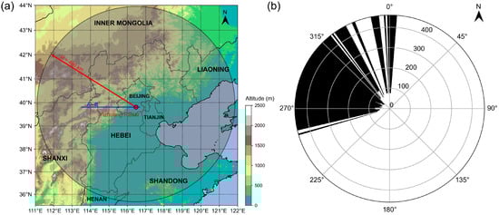
Figure 1.
Details of the Yizhuang S-band radar. (a) The location and the detection range of the Yizhuang radar. (b) Beam blockage range at 0.5° of the Yizhaung radar. The radar observations at the elevation angle of 0.5° are totally blocked in the black areas from the azimuth of 255° to 5°, while in the white areas, the 0.5° observations are available.
To help understand the data-missing problem caused by beam blockage more intuitively, we plotted a rough zonal terrain profile along the latitude line passing through the Yizhuang radar (the blue line in Figure 1a, marked with “A,B”), which depicts the topography along the profile and the blockage of radar beams (Figure 2). For radar beams of higher elevation angles, such as 1.5° and 2.5°, the radar beams will never be blocked by the terrain, so the observations at these elevation angles are visible. However, radar beams of 0.5° will be blocked by a mountain with the local maximum altitude point near the radar site, which leads to a large blocked area behind the mountains and a short visible radial distance in front of the mountains.
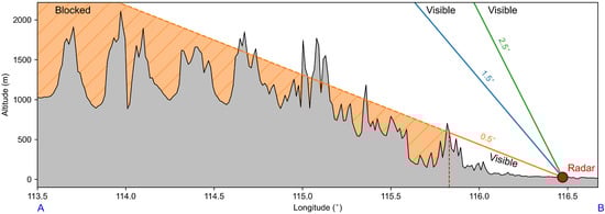
Figure 2.
A rough zonal terrain profile along the latitude line passing through the Yizhuang radar. The location of the Yizhuang radar is marked with a red circle. The terrain along the profile is drawn in black lines and filled in grey. The radar beams are represented by orange, blue, and green lines, corresponding to the elevation angles of 0.5°, 1.5°, and 2.5°, respectively. The orange dashed line and the orange-filled region illustrate that radar beams of 0.5° are blocked by the mountain peak near the radar site, leading to a large data-missing area.
3. Methods
3.1. Model Architecture
The architecture of DSA-UNet is illustrated in Figure 3. The model follows the U-Net structure, which can be divided into an encoder and a decoder. The encoder accepts the multi-elevation reflectivity and the corresponding mask as its input (orange rectangle), which are compressed into a tensor with the shape of (channel, height, and width). The input tensor is processed with a feature recombination block (1 × 1 convolution, orange arrows) before being fed into four sequential downscaling blocks (red arrows). The feature maps are halved in dimensions H and W and doubled in dimension C through every downscaling block. The downscaling blocks are followed by four dilated convolution blocks (violet arrows) to capture the multi-scale information aggregation of the encoding feature maps [30]. The decoder consists of four upscaling blocks (green arrows) and a 1 × 1 convolution block (orange arrow), similar to the encoder. One difference is that the decoding feature maps of the first two upscaling blocks are processed with two additional self-attentional blocks (black arrows) to learn patterns using cues from all feature locations for image generation or completion [31]. Each decoding feature map is concatenated by the encoding feature map of an equal scale copied from the encoder through skip connections (grey arrows). The sizes of encoding and decoding feature maps are also marked out next to the rectangles, which will be explained in the following subsection. The DSA-UNet model has about 18.17 million trainable parameters in total.
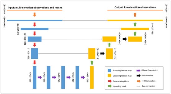
Figure 3.
The architecture of DSA-UNet. The intermediate feature maps, scaling blocks, and other modules are represented with rectangles and arrows in corresponding colors. The legend can be found in the lower right corner.
The structures of the downscaling blocks and upscaling blocks are shown in Figure 4. The downscaling blocks consist of double convolutional blocks, each including a 3 × 3 convolution layer, a batch normalization (BN) layer, and a rectified linear unit (ReLU) layer. The first 3 × 3 convolution layer serves as the downscaling operator, which reshapes the input tensor from to . The feature maps keep the same size in the following layers. The upscaling operation in the upscaling blocks is implemented by a 3 × 3 transpose convolution layer instead of the 3 × 3 convolution layer in downscaling blocks.
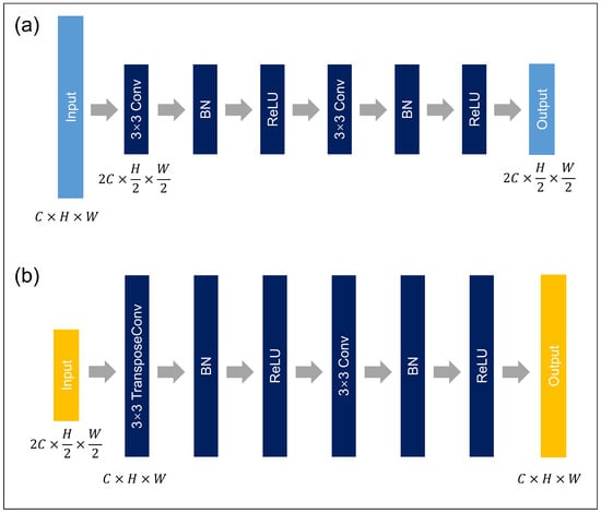
Figure 4.
The structures of the downscaling blocks (a) and upscaling blocks (b). The light-blue and yellow rectangles denote the input and output feature maps, and the dark-blue rectangles denote the neural network layers.
The structure of the self-attentional blocks is shown in Figure 5. The input tensor is flattened and fed into three independent 1 × 1 convolution layers. The feature maps of the first two convolution layers are combined through a dot product and a softmax layer to generate an attention map that records a full relationship between all pixels in the spatial dimensions. It is then multiplied by the feature map from the last 1 × 1 convolution and transferred to the original size.
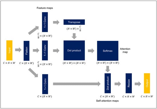
Figure 5.
The structure of the self-attentional blocks. The yellow rectangles denote the input and output feature maps, and the dark-blue rectangles denote the neural network layers.
3.2. Data Processing and Dataset Construction
The radar raw data were first processed with a quality control process, which is always implemented in weather monitoring applications to eliminate systematic observation errors of radars. The processed radar data had a minimum value of −33 dBZ, which indicates clear air, and a maximum value of 69 dBZ, which indicates an extreme amount of precipitation particles. The processed radar reflectivity values were clipped between 0 and 70 dBZ and scaled to the range of 0–1 with the linear min–max normalization. The lower bound of the min–max normalization was 0 dBZ because, according to several Z-R relations, when the radar reflectivity is lower than 0 dBZ, the estimated precipitation is lower than 0.1 mm, which can be regarded as none precipitation [32]. This clipping operation has also been applied in some related studies [28,33]. As we introduced in Section 2, the original radar data have a size of 360° × 460 km with a resolution of 1° × 1 km in the polar coordinate system centered at the Yizhuang radar site. Considering that the radar beams broaden with distance and altitude and the phase of precipitation particles changes above the melting layer [10], the radar data are restricted to a maximum distance of 80 km and a maximum elevation angle of 3.5°.
The dataset for training and evaluation is built based on radar data of 1.5°, 2.5°, and 3.5° because the data quality of 0.5° observations is limited by considerable beam blockage. Observations at these three elevation angles are inputted into the model, and the 1.5° observations are set as the training target. To simulate varying degrees of data-missing situations, a series of random sector masks are generated for the 1.5° observations, where the values of each mask are filled with zero in data-missing regions and one elsewhere. The location of the masked area is randomly determined for each 1.5° observation. The azimuthal distance of the masked area is also randomly sampled from 10° to 40°. The radial distance of the mask is fixed to 80 km. The random sector mask is also regarded as part of the input to provide necessary information about the locations of missing pixels for the neural network. The model’s output is split by the mask and merged with the input, which can be described by
where and represent the input radar image tensor and the mask; represents the neural network; and represent the raw output and the final output of the neural network; and the symbol ⊙ represents the element-wise product operation. Besides the mask of the 1.5° observation, two additional masks filled with one were also fed into the neural network to let it understand that the 2.5° and 3.5° radar observations serve as auxiliary information but not the training target. The channel sizes of the input and output tensors are 6 and 1, respectively.
In deep learning tasks, structured data are usually converted into a tensor format in a Cartesian coordinate system for convolutional neural networks. This is reasonable for convolution operations in most image completion tasks because of the translation invariance in convolution operators, while for the polar coordinate system, where the elements are in sequential order along the azimuth direction, the head (0°) and the tail (359°) elements are geographically adjacent but are far apart from each other in the tensor. Therefore, an additional padding operation to both the head and the tail of the tensor is necessary. For a tensor at a certain time step, the elements within 0°–20° are attached to the tail of the tensor; meanwhile, those within 339°–359° are padded before the head, which indicates that the azimuthal size of the tensor is expanded to 400. The radial size of the tensor is 80 since its radial distance is 80 km and its radial resolution is 1 km. Therefore, the full sizes of the input tensor and the output tensor are 6 × 400 × 80 and 1 × 400 × 80, respectively, as shown in Figure 3.
The random sector masks were also used to augment the dataset for better training. Each 1.5° observation is linked to four random sector masks with different locations and ranges. In this way, the size of the dataset was expanded to 4 times the original size. The augmented dataset with a total of 70,664 samples was sorted in chronological order and was then split into the training set (45,225 samples), validation set (11,306 samples), and test set (14,133 samples).
3.3. Baseline Methods
The multivariate linear regression (MLG) method, the bilinear interpolation (BI) method, and the UNet++ GAN model were selected as the baseline methods. The MLG method is one of the most basic statistical methods for multivariate correlation analysis. The BI method is a non-parametric statistical interpolation method for multi-dimensional variables, which is widely used in image processing. The UNet++ GAN model directly aims at the radar data completion task, which was designed based on the conditional generative adversarial network [34] and UNet++ [35].
For the MLG method, observations from all the elevation angles that are above 1.5° (including 2.5°, 3.5°, 4.5°, 6.0°, 10.0°, 15.0°, and 19.5°) were used to fit the 1.5° observations. For the BI method, the unmasked values in the 1.5° observations served as the source for interpolating masked values. The UNet++ GAN model shares the same dataset and input–output settings as the DSA-UNet model. Its architectures and details can be found in [28].
3.4. Training
The original L1 loss function is a commonly used training goal for deep learning models, which is defined as the average of the absolute difference between the prediction and the observation. It usually works when the data follow a balanced or regular distribution, for example, a Gaussian distribution. However, the dataset in this study was not in this condition. According to the principle of Doppler weather radars, observations with higher radar reflectivity are usually instructive to heavier precipitation or more fierce storm events. Although the data were collected during rainy days in warm seasons, the number of high-intensity values was significantly fewer than that of low-intensity values, causing the dataset to be highly unbalanced. Figure 6 describes the distribution of the raw radar reflectivity data. It can be observed that the density of radar reflectivity values over 40 dBZ was significantly less than that of values below 10 dBZ. Since the original L1 loss function was unsuitable for the highly unbalanced dataset, we designed a weighted L1 loss function for training the DSA-UNet model to overcome this problem, as shown in Equation (2). The weighted L1 loss of the prediction () and the observation () is scaled by the weight () determined by the observation’s value. Larger weights are set for intervals with higher intensity but lower distribution density based on the characteristics of the data distribution. The correspondence between the radar reflectivity values and the weights is exhibited in Figure 6.
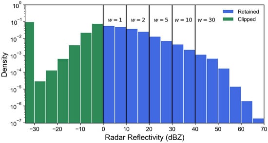
Figure 6.
The distribution histogram of the raw radar reflectivity data. The green bar indicates that values below 0 dBZ were clipped, while the blue bar indicates that values between 0 and 70 dBZ were retained. The weights of the L1 loss function for different intervals were placed above the bars.
The learnable parameters of each layer in the DSA-UNet model were initialized with the default initialization scheme and then trained by an Adam optimizer [36] with a learning rate of 0.0001 and a max iteration of 100,000. The parameters of the DSA-UNet were updated via backpropagation after each iteration with the mini-batch training skill. The dataset was segmented into mini-batches with a size of 32. The validation set with 11,306 samples was employed for optimal parameter selection. The early stopping training skill and the L2 regularization were adopted to avoid the overfitting of the neural network. The generators and discriminators of the UNet++ GAN model shared the optimizer, the learning rate, and the mini-batch size. It was trained using a combination of the original GAN loss and the weighted L1 loss. The optimal parameters of the MLG method were also approximated with an Adam optimizer because the dataset was too large for directly computing the theoretical solution. All of the experiments in this study were implemented on an Nvidia Tesla A100 graphic card based on the open-source machine learning framework PyTorch. Other detailed settings are listed in Table 1.

Table 1.
Training settings of the DSA-UNet model, the UNet++ GAN model, and the MLG method. The non-parametric BI method is not included.
3.5. Evaluation Metrics
Since the aim of this study is to better complete the missing regions of the radar observations, the evaluation metrics should be capable of measuring the differences between the predicted values and the observed values in the masked areas. The mean bias error (MBE), the mean absolute error (MAE), and the root mean squared error (RMSE) are popular evaluation metrics for estimating the differences or bias. However, since the area of the annular sector grows rapidly as the radial distance increases, the evaluation metrics must take the variability of pixel area into consideration. The above metrics were weighted by a tensor determined by the areas of the annular sectors at different radial distances, as defined in Equation (3). The weighted metrics (WMBE, WMAE, and WRMSE) were selected as the evaluation metrics, which are defined in Equations (4)–(6).
In the above equations, represents the observation and represents the prediction; represents the sector mask; ⊙ represents the Hadamard product; the operator represents the sum operation along the radial () and the azimuthal () axis; and R and are the sizes of radial range (80) and azimuthal range (400 for DL models and 360 for traditional methods). The weight tensor meets the condition of . Considering the unbalance of the dataset, we selected 10, 20, 30, 40, and 50 dBZ as the thresholds for the above metrics to better evaluate the bias in different radar reflectivity intervals.
In addition to the above metrics, we selected the PPI plots, the contrast scatter (CS) plots, and the power spectral density (PSD) plots as evaluation methods for further analysis. The PPI plot is a radar display that gives a conical section of radar observations at a certain elevation angle. The CS plot describes the correlation between the predicted values and the observed values. The PSD plot presents the relationship between the power and frequency of a signal, which was used in radar nowcasting studies to evaluate the performance of representing diverse-scale weather patterns [22,23]. The above metrics and plots were also used for model evaluation in related studies [10,28,33].
4. Results
4.1. Performance on the Test Set
The overall data completion performance of the DSA-UNet and its baseline models was evaluated on the test set with a total of 14,133 samples. The WMAE, WRMSE, and WMBE of the models in different radar reflectivity intervals were calculated and are illustrated in Figure 7. It can be observed that the MLG method produced the highest overall WMAE and WRMSE, as well as the lowest overall WMBE that was far below zero, implying a severe systematic underestimation problem. The BI method’s systematic error indicated by the WMBE was lower than the MLG method, and so did its absolute error indicated by the WMAE and the WRMSE. DL models (UNet++ GAN and DSA-UNet) performed better than the MLG method and the BI method when comparing the overall metrics. Among all of the models, the DSA-UNet reached the lowest overall WMAE, the lowest overall WRMSE, and the nearest overall WMBE to zero, which indicated that the DSA-UNet could generate a lower error between its predictions and the observations than the other baseline models.
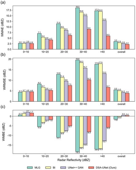
Figure 7.
The evaluation metrics of the models on the test set. The horizontal axis represents different radar reflectivity intervals and the overall performance. The vertical axis represents the evaluation metrics, including WMAE (a), WRMSE (b), and WMBE (c).
The evaluation metrics for different radar reflectivity intervals were also illustrated in Figure 7. Generally, the results show that the DL models and the traditional methods performed the best for radar reflectivity in 0–10 dBZ, but the worst in 30–40 dBZ, where all of them met a notable systematic underestimation. Their errors were close to each other when the radar reflectivity was low (0–20 dBZ). Specifically, the MLG method and the BI method had even lower errors than DL models for radar reflectivity in 0–10 dBZ. However, when the radar reflectivity exceeded 20 dBZ, the errors of the baseline methods grew rapidly as the radar reflectivity increased. Their performance became considerably worse when the radar reflectivity was higher than 30 dBZ. Compared to the baseline methods, the DSA-UNet model achieved significantly lower WMAE and WRMSE as well as the absolute value of WMBE, especially for high radar reflectivity values, which suggests that it had a lower systematic error and a lower absolute bias than its baseline methods.
4.2. Case Study
The data completion performance of the DSA-UNet and its baseline models was also evaluated and further analyzed with two cases that were selected from the test set. Case 1 was selected from a moderate-intensity widespread rainfall event at 13:00 UTC on 22 July 2019. Case 2 was selected from a high-intensity squall line event at 15:00 UTC on 6 August 2019. The evaluation was implemented only for the masked areas.
4.2.1. Case 1
The PPI images of the 1.5° radar reflectivity observation and the predictions generated by the DSA-UNet and its baseline models for Case 1 are shown in Figure 8. The azimuthal boundaries of the sector mask for Case 1 were set as 315° and 355°, which were marked with dashed lines. The PPI image of the observation shows that the observed radar reflectivity of the masked area was mostly between 20 and 40 dBZ. The azimuthal boundaries of the sector mask for Case 1 were set as 270° and 310°, which were marked with dashed lines. The PPI image of the observation (Figure 8a) shows that the observed radar reflectivity of the masked area was mostly between 20 and 40 dBZ. It can be found that the radar reflectivity values predicted by the MLG method (Figure 8b) were significantly lower than the observed values, implying a severe systematic underestimation. The prediction of the BI method (Figure 8c) in the masked area showed an abnormal striped feature that did not exist in the observation. This was because when the beams in the radial direction were completely blocked, the values were interpolated merely along the azimuthal direction based on the visible values outside the mask boundaries. The predictions of the DL models were closer to the observation compared to the MLG method and the BI method. However, the predictions of the UNet++ GAN model (Figure 8d) had fewer local-scale patterns than the observation, or to be more intuitive, its prediction was smoother and blurrier. The prediction of the DSA-UNet model (Figure 8e) was the closest to the observation. It not only had the most similar reflectivity shape to the observation but also had the richest local-scale details. The merged PPI image of the DSA-UNet model’s prediction also appeared more seamless, which indicates that the predicted values in the masked area and the observed values in the unmasked area were intensely close.
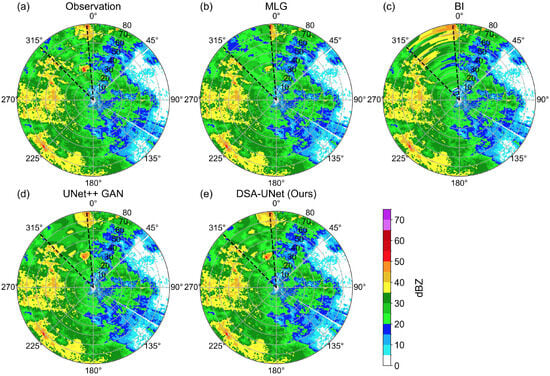
Figure 8.
The PPI images of the 1.5° radar reflectivity observation and the predictions for Case 1. (a) Observation; (b) prediction of MLG; (c) Prediction of BI; (d) prediction of UNet++ GAN; (e) prediction of DSA-UNet. The boundaries of the sector mask are marked with dashed lines.
Figure 9 shows the evaluation metrics of the models for Case 1. The results show that the BI method had the highest overall systematic error and absolute error, especially for radar reflectivity over 30 dBZ. The MLG method produced the second-highest systematic error absolute error. Its performance was limited by a systematic underestimation of high radar reflectivity values that were over 30 dBZ. The overall error of the UNet++ GAN model was lower than the traditional methods but was higher than the DSA-UNet model. The UNet++ GAN model had the worst performance for radar reflectivity below 10 dBZ, but it significantly exceeded the traditional methods for high radar reflectivity. The DSA-UNet model achieved the best performance for most radar reflectivity intervals except 0–10 dBZ where it was a bit inferior to the BI method.
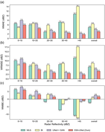
Figure 9.
The evaluation metrics of the models for Case 1. The horizontal axis represents different radar reflectivity intervals and the total performance. The vertical axis represents the evaluation metrics, including WMAE (a), WRMSE (b), and WMBE (c).
Figure 10 shows the CS plot of the observed and predicted values in the masked areas for Case 1. In a CS plot, the horizontal axis and the vertical axis represent the observation and the prediction, respectively. The points on the 45° line imply perfect predictions, yet the points below or beyond this line signify underestimations or overestimations. The colors of the points are determined with the probability density provided by the Gaussian kernel density estimation. The results show that most of the observation values lay in the range of 20–40 dBZ, which is consistent with Figure 8. The MLG method (Figure 10a) and the BI method (Figure 10b) were limited by a significant underestimation and a high prediction variance, respectively. The scatters of the UNet++ GAN model (Figure 10c) and the DSA-UNet model (Figure 10d) were distributed closer to the 45° line, indicating their better performance than traditional methods. The scatters of the DSA-UNet model were more tightly concentrated on the 45° line than the UNet++ GAN model, which indicates that the DSA-UNet model could achieve a lower prediction systematic error and variance for Case 1. It can also be found that the DL models tended to overestimate low radar reflectivity values in 0–10 dBZ, which is consistent with Figure 9.
Figure 10.
The CS plot of the observed and predicted values in the masked areas for Case 1. (a) MLG; (b) BI; (c) UNet++ GAN; (d) DSA-UNet.
To further explain the above results, we plotted the PSDs of the observation and predictions along the radial and azimuthal axes in the masked areas for Case 1, as shown in Figure 11. In this study, the horizontal axis of the PSD plot represents the spatial wavelength, which is positively correlated with the spatial scale. The vertical axis represents the PSD at certain spatial wavelengths. A higher PSD generally indicates richer local details when the spatial wavelength is short. Generally, both radial and azimuthal PSDs decrease as the spatial wavelength reduces. When the spatial wavelength is long (over 16 km or 16°), the radial and azimuthal PSDs of the DL models’ predictions were closer to the PSD of the observation than those of the MLG method and the BI method. When the spatial wavelength is shorter than 4 km or 4°, the PSDs of the MLG method exceeded the PSDs of the DL models. The radial PSD of the BI method is significantly dissimilar to the azimuthal PSD due to a lack of radial information. The DSA-UNet model reached a higher PSD than the UNet++ GAN model, especially at short spatial wavelengths, indicating that the DSA-UNet model had a better capability of reconstructing local-scale spatial patterns, which is consistent with the results in the PPI plot and the CS plot.
Figure 11.
The PSD plot of the observation and predictions in the masked areas for Case 1. (a) Radial PSD; (b) azimuthal PSD.
4.2.2. Case 2
The PPI images of the observation and the predictions for Case 2 are shown in Figure 12. The sector mask covered an azimuthal range of 40°–80°. Figure 12a shows that a local high-intensity radar echo region was located in the northeast of the masked area, with a maximum reflectivity of over 50 dBZ, while in the remaining part of the masked area, the radar reflectivity was much lower (below 10 dBZ). The MLG method (Figure 12b) and the BI method (Figure 12c) met the systematic underestimation and striped pattern problems, respectively, which were also found in Case 1. The DL models made better predictions than the above two methods in the aspect of both general echo intensity and shape. The DL models made better predictions than the above two methods in the aspect of both general echo intensity and shape. The UNet++ GAN model (Figure 12d) fell behind the DSA-UNet model (Figure 12e) in predicting the location of the peak value.
Figure 12.
The PPI images of the 1.5° radar reflectivity observation and the predictions for Case 2. (a) Observation; (b) prediction of MLG; (c) prediction of BI; (d) prediction of UNet++ GAN; (e) prediction of DSA-UNet. The boundaries of the sector mask are marked with dashed lines.
Figure 13 shows the evaluation metrics of the predictions of the models for Case 2. Similar to Case 1, the BI method had the highest overall prediction error in all of the metrics (WMAE, WRMSE, and WMBE), especially when the radar reflectivity was over 40 dBZ. The performance of the MLG method was also unacceptable due to its high bias and underestimation of high radar reflectivity. In contrast to the traditional methods, both DL models could produce better overall performance. However, the performance of the UNet++ GAN model was inferior to the MLG method when the radar reflectivity was below 20 dBZ. Instead, the DSA-UNet model achieved a lower systematic and absolute error for both high and low radar reflectivity than all of the other baseline models.
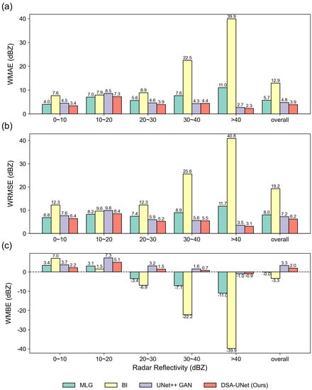
Figure 13.
The evaluation metrics of the models for Case 2. The horizontal axis represents different radar reflectivity intervals and the total performance. The vertical axis represents the evaluation metrics, including WMAE (a), WRMSE (b), and WMBE (c).
Figure 14 displays the CS plot of the observed and predicted values in the masked areas for Case 2. Different from Case 1, the radar reflectivity values of the observation in Case 2 were mainly clustered in the 0–10 dBZ. Meanwhile, the amount of observed values over 50 dBZ in Case 2 was larger. The scatters of the MLG method (Figure 14a) deviated from the 45° line, especially for observed values that were over 30 dBZ, indicating the aforementioned underestimation problem for high-intensity radar data completion. The scatters of the BI method (Figure 14b) were dispersed over the entire radar reflectivity value ranges, which confirms its poor performance, as shown in Figure 12 and Figure 13. The scatters of the UNet++ GAN model (Figure 14c) were more centered around the 45° line, but this model tended to overestimate the values. The DSA-UNet model (Figure 14d) produced a better prediction than the other baseline models. The scatters of the DSA-UNet model were the most concentrated in the 45° line and had the highest cluster density (dark-red points). This model also had a systematic overestimation for low radar reflectivity values (below 10 dBZ), but this problem was remarkably alleviated for moderate and high radar reflectivity (over 20 dBZ).
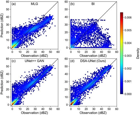
Figure 14.
The CS plot of the observed and predicted values in the masked areas for Case 2. (a) MLG; (b) BI; (c) UNet++ GAN; (d) DSA-UNet.
The radial and azimuthal PSDs of the predictions and the observation in the masked area for Case 2 were calculated and exhibited in Figure 15. Similar to Case 1, the MLG method achieved the highest radial and azimuthal PSD among all of the methods. The azimuthal PSD of the BI method is significantly lower than the other models. Meanwhile, the radial PSD of the BI method oscillates as the radial wavelength reduces due to a lack of radial information. The UNet++ GAN model performed the worst, particularly for short spatial wavelengths that imply local-scale patterns. The DSA-UNet model achieved higher radial and azimuthal PSDs than the UNet++ GAN model, which indicates that this model was more qualified for capturing and completing diverse-scale patterns in data-missing areas. However, there is still a gap between the PSDs of the DSA-UNet model and the MLG method for very short spatial wavelengths.
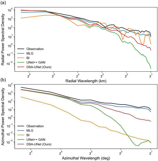
Figure 15.
The PSD plot of the observation and predictions in the masked areas for Case 2. (a) Radial PSD; (b) azimuthal PSD.
5. Discussion
In Section 4, the data completion performance of our proposed DSA-UNet model was evaluated on the entire test set and further analyzed with two cases, where the model was also compared with the MLG method, the BI method, and the UNet++ GAN model. The evaluation methods consisted of three quantitative metrics (WMBE, WMAE, and WRMSE) and three diagrams (PPI plot, CS plot, and PSD plot) for further analysis of the case study.
Generally, the quantitative evaluation results revealed that the DL models performed better than the traditional methods. The MLG method benefited from its simple principle and strong interpretability, which was based on the assumption that the radar reflectivity values at different elevation angles were linearly correlated. However, the MLG method ran into a systematic underestimation problem, especially for areas with high radar reflectivity values, which made it unsuitable for completing radar observations in heavy rainfall scenarios. The non-parametric BI method was found to suffer from a striped pattern problem that caused the method to fail in high-reflectivity data completion. Compared to the traditional methods, the general errors between the DL models’ predictions and the observations were significantly lower; the predicted intensity and position of high-value areas were also more accurate.
It was also revealed that the DSA-UNet model could bring improvements to radar missing data completion over the current DL model proposed in previous research. Compared to the UNet++ GAN model, the DSA-UNet model achieved better performance on both the entire test and the case study. It provided the completion closer to the real observation in almost all radar reflectivity intervals, especially for extreme values, which play an important role in signifying severe storms. The PPI and PSD diagrams in the case study illustrated that the DSA-UNet model could improve the modeling and reconstruction of local-scale radar echo patterns over the UNet++ GAN model. These improvements were possibly facilitated by the dilated convolutional modules and self-attentional modules in the DSA-UNet model, which could strengthen the model’s ability to learn local and subtle information from the data. The improvements of the DSA-UNet model over the baseline models are beneficial for finer weather monitoring.
Although the DSA-UNet model has shown a surpassing performance over the baseline models in weather radar data completion, it still meets several limitations. The quantitative results and the CS diagrams revealed that the DSA-UNet model tended to slightly overestimate low radar reflectivity values, especially for values below 10 dBZ, which was similar to the UNet++ GAN model. Under this overestimation, the model has the potential to involve abnormal clutters when completing missing data. Furthermore, the PSD diagrams indicated that although the DSA-UNet was able to narrow the gap between the predicted and observed radar reflectivity values in local-scale radar echo patterns, it still lagged behind traditional statistical methods, suggesting that there is still room for improvement. The above drawbacks were also noticed and summarized as the blurry effect of DL models in studies on precipitation nowcasting [22,23,37]. The improving methods proposed in these studies might be constructive for eliminating the drawbacks of the DSA-UNet model. Moreover, the data in this study were collected only from warm seasons, which were mainly composed of convective precipitation samples instead of stratiform precipitation samples. Meanwhile, the lowest elevation angle of the radar data for the experiments was selected as 1.5° instead of 0.5°, which was unavailable because of severe beam blockage and noises. The generalization of the DSA-UNet model to different precipitation types and lower elevation angles still needs further assessment.
6. Conclusions
The data-missing problem is one of the major factors that limit the quality of weather radar data and subsequent applications. Traditional solutions based on radar physics and statistics in previous studies have shown obvious defects in various aspects. Researchers have applied deep learning (DL) techniques to the completion of weather radar missing data, but their methods were limited by low accuracy. In this study, we proposed a dilated and self-attentional UNet (DSA-UNet) model to improve the completion quality of weather radar missing data. The model was trained and evaluated on a radar dataset built from the Yizhuang radar observations during the warm seasons from 2017 to 2019. It was further analyzed with two cases based on three quantitative metrics (WMBE, WMAE, and WRMSE) and three diagrams (PPI plot, CS plot, and PSD plot). Several baseline methods and models were selected and compared with our proposed DSA-UNet model, including the MLG method, the BI method, and the UNet++ GAN model. The major findings of this study are as follows:
- The DL models can outperform traditional statistical methods by reducing the general errors between their predictions and the observation and by predicting the intensity and position of high radar reflectivity values more accurately.
- Compared to the UNet++ GAN model, the DSA-UNet model can produce a better completion that is closer to the real observation in almost all radar reflectivity intervals, especially for extreme values.
- The DSA-UNet model can better capture and reconstruct local-scale radar echo patterns over the UNet++ GAN model.
- The limitations of the DSA-UNet model include the slight underestimation of low values and the local-scale details.
This study provides an effective solution for improving the completion of weather radar missing data and also reveals the great potential of deep learning in weather radar applications. Future studies will improve the network architecture to eliminate the current drawbacks and incorporate radar data that contain various precipitation types and lower elevation angles to assess the generalization of our method.
Author Contributions
Conceptualization, A.G. and G.N.; methodology, A.G.; software, A.G.; validation, A.G.; formal analysis, A.G.; investigation, A.G.; resources, A.G.; data curation, A.G.; writing—original draft preparation, A.G.; writing—review and editing, H.C. and G.N.; visualization, A.G.; supervision, G.N.; project administration, G.N.; funding acquisition, G.N. All authors have read and agreed to the published version of the manuscript.
Funding
This work was supported by the National Key Research and Development Program of China (2022YFC3090604) and the Fund Program of State Key Laboratory of Hydroscience and Engineering (61010101221).
Data Availability Statement
The data in this study is unavailable due to privacy restrictions. The codes for the experiments are available at https://github.com/THUGAF/Radar-Completion (accessed on 14 September 2023).
Acknowledgments
The authors gratefully acknowledge the anonymous reviewers for providing careful reviews and comments on this article.
Conflicts of Interest
The authors declare no conflict of interest.
Abbreviations
The following abbreviations are used in this manuscript:
| CINRAD | China Next Generation Weather Radar |
| VPR | Vertical profile of radar reflectivity |
| DEM | Digital elevation model |
| DL | Deep learning |
| DSA | Dilated and self-attentional |
| MLG | Multivariate linear regression |
| BI | Bilinear interpolation |
| GAN | Generative adversarial network |
| MBE | Mean bias error |
| MAE | Mean absolute error |
| RMSE | Root mean squared error |
| WMBE | Weighted mean bias error |
| WMAE | Weighted mean absolute error |
| WRMSE | Weighted root mean squared error |
| PPI | Plan position indicator |
| CS | Contrast scatter |
| PSD | Power spectral density |
References
- Agrawal, S.; Barrington, L.; Bromberg, C.; Burge, J.; Gazen, C.; Hickey, J. Machine Learning for Precipitation Nowcasting from Radar Images. arXiv 2019, arXiv:1912.12132. [Google Scholar]
- Brown, R.A.; Wood, V.T.; Barker, T.W. Improved detection using negative elevation angles for mountaintop WSR-88Ds: Simulation of KMSX near Missoula, Montana. Weather Forecast. 2002, 17, 223–237. [Google Scholar] [CrossRef]
- Wood, V.T.; Brown, R.A.; Vasiloff, S.V. Improved detection using negative elevation angles for mountaintop WSR-88Ds. Part II: Simulations of the three radars covering Utah. Weather Forecast. 2003, 18, 393–403. [Google Scholar] [CrossRef]
- Germann, U.; Boscacci, M.; Clementi, L.; Gabella, M.; Hering, A.; Sartori, M.; Sideris, I.V.; Calpini, B. Weather radar in complex orography. Remote Sens. 2022, 14, 503. [Google Scholar] [CrossRef]
- Min, C.; Chen, S.; Gourley, J.J.; Chen, H.; Zhang, A.; Huang, Y.; Huang, C. Coverage of China new generation weather radar network. Adv. Meteorol. 2019, 2019, 5789358. [Google Scholar] [CrossRef]
- Vignal, B.; Galli, G.; Joss, J.; Germann, U. Three methods to determine profiles of reflectivity from volumetric radar data to correct precipitation estimates. J. Appl. Meteorol. Climatol. 2000, 39, 1715–1726. [Google Scholar] [CrossRef]
- Andrieu, H.; Creutin, J.D. Identification of vertical profiles of radar reflectivity for hydrological applications using an inverse method. Part I: Formulation. J. Appl. Meteorol. Climatol. 1995, 34, 225–239. [Google Scholar] [CrossRef]
- Vignal, B.; Andrieu, H.; Creutin, J.D. Identification of vertical profiles of reflectivity from volume scan radar data. J. Appl. Meteorol. Climatol. 1999, 38, 1214–1228. [Google Scholar] [CrossRef]
- Joss, J.; Pittini, A. Real-time estimation of the vertical profile of radar reflectivity to improve the measurement of precipitation in an Alpine region. Meteorol. Atmos. Phys. 1991, 47, 61–72. [Google Scholar] [CrossRef]
- Yin, X.; Hu, Z.; Zheng, J.; Li, B.; Zuo, Y. Study on Radar Echo-Filling in an Occlusion Area by a Deep Learning Algorithm. Remote Sens. 2021, 13, 1779. [Google Scholar] [CrossRef]
- Bech, J.; Codina, B.; Lorente, J.; Bebbington, D. The sensitivity of single polarization weather radar beam blockage correction to variability in the vertical refractivity gradient. J. Atmos. Ocean. Technol. 2003, 20, 845–855. [Google Scholar] [CrossRef]
- Lang, T.J.; Nesbitt, S.W.; Carey, L.D. On the correction of partial beam blockage in polarimetric radar data. J. Atmos. Ocean. Technol. 2009, 26, 943–957. [Google Scholar] [CrossRef]
- Bech, J.; Gjertsen, U.; Haase, G. Modelling weather radar beam propagation and topographical blockage at northern high latitudes. Q. J. R. Meteorol. Soc. J. Atmos. Sci. Appl. Meteorol. Phys. Oceanogr. 2007, 133, 1191–1204. [Google Scholar] [CrossRef]
- Shakti, P.; Maki, M.; Shimizu, S.; Maesaka, T.; Kim, D.S.; Lee, D.I.; Iida, H. Correction of reflectivity in the presence of partial beam blockage over a mountainous region using X-band dual polarization radar. J. Hydrometeorol. 2013, 14, 744–764. [Google Scholar]
- Andrieu, H.; Creutin, J.; Delrieu, G.; Faure, D. Use of a weather radar for the hydrology of a mountainous area. Part I: Radar measurement interpretation. J. Hydrol. 1997, 193, 1–25. [Google Scholar] [CrossRef]
- Creutin, J.; Andrieu, H.; Faure, D. Use of a weather radar for the hydrology of a mountainous area. Part II: Radar measurement validation. J. Hydrol. 1997, 193, 26–44. [Google Scholar] [CrossRef]
- Yoo, C.; Park, C.; Yoon, J.; Kim, J. Interpretation of mean-field bias correction of radar rain rate using the concept of linear regression. Hydrol. Process. 2014, 28, 5081–5092. [Google Scholar] [CrossRef]
- Kvasov, R.; Cruz-Pol, S.; Colom-Ustáriz, J.; Colón, L.L.; Rees, P. Weather radar data visualization using first-order interpolation. In Proceedings of the 2013 IEEE International Geoscience and Remote Sensing Symposium-IGARSS, Melbourne, Australia, 21–26 July 2013; pp. 3574–3577. [Google Scholar]
- Foehn, A.; Hernández, J.G.; Schaefli, B.; De Cesare, G. Spatial interpolation of precipitation from multiple rain gauge networks and weather radar data for operational applications in Alpine catchments. J. Hydrol. 2018, 563, 1092–1110. [Google Scholar] [CrossRef]
- Li, B.; Li, R.; Sun, T.; Gong, A.; Tian, F.; Khan, M.Y.A.; Ni, G. Improving LSTM hydrological modeling with spatiotemporal deep learning and multi-task learning: A case study of three mountainous areas on the Tibetan Plateau. J. Hydrol. 2023, 620, 129401. [Google Scholar] [CrossRef]
- Shi, X.; Chen, Z.; Wang, H.; Yeung, D.Y.; Wong, W.K.; Woo, W.C. Convolutional LSTM network: A machine learning approach for precipitation nowcasting. In Proceedings of the Advances in Neural Information Processing Systems, Montreal, ON, Canada, 7–12 December 2015; pp. 802–810. [Google Scholar]
- Ravuri, S.; Lenc, K.; Willson, M.; Kangin, D.; Lam, R.; Mirowski, P.; Fitzsimons, M.; Athanassiadou, M.; Kashem, S.; Madge, S.; et al. Skilful precipitation nowcasting using deep generative models of radar. Nature 2021, 597, 672–677. [Google Scholar] [CrossRef]
- Ayzel, G.; Scheffer, T.; Heistermann, M. RainNet v1.0: A convolutional neural network for radar-based precipitation nowcasting. Geosci. Model Dev. 2020, 13, 2631–2644. [Google Scholar] [CrossRef]
- Sadeghi, M.; Asanjan, A.A.; Faridzad, M.; Nguyen, P.; Hsu, K.; Sorooshian, S.; Braithwaite, D. PERSIANN-CNN: Precipitation estimation from remotely sensed information using artificial neural networks–convolutional neural networks. J. Hydrometeorol. 2019, 20, 2273–2289. [Google Scholar] [CrossRef]
- Pan, B.; Hsu, K.; AghaKouchak, A.; Sorooshian, S. Improving precipitation estimation using convolutional neural network. Water Resour. Res. 2019, 55, 2301–2321. [Google Scholar] [CrossRef]
- Afzali Gorooh, V.; Kalia, S.; Nguyen, P.; Hsu, K.l.; Sorooshian, S.; Ganguly, S.; Nemani, R.R. Deep neural network cloud-type classification (DeepCTC) model and its application in evaluating PERSIANN-CCS. Remote Sens. 2020, 12, 316. [Google Scholar] [CrossRef]
- Song, T.; Li, Y.; Meng, F.; Xie, P.; Xu, D. A novel deep learning model by Bigru with attention mechanism for tropical cyclone track prediction in the Northwest Pacific. J. Appl. Meteorol. Climatol. 2022, 61, 3–12. [Google Scholar]
- Geiss, A.; Hardin, J.C. Inpainting radar missing data regions with deep learning. Atmos. Meas. Tech. 2021, 14, 7729–7747. [Google Scholar] [CrossRef]
- Ronneberger, O.; Fischer, P.; Brox, T. U-net: Convolutional networks for biomedical image segmentation. In Proceedings of the International Conference on Medical Image Computing and Computer-Assisted Intervention, Munich, Germany, 5–9 October 2015; Springer: Berlin/Heidelberg, Germany, 2015; pp. 234–241. [Google Scholar]
- Yu, F.; Koltun, V. Multi-scale context aggregation by dilated convolutions. arXiv 2015, arXiv:1511.07122. [Google Scholar]
- Zhang, H.; Goodfellow, I.; Metaxas, D.; Odena, A. Self-attention generative adversarial networks. In Proceedings of the International Conference on Machine Learning, Long Beach, CA, USA, 9–15 June 2019; PMLR: Cambridge, MA, USA, 2019; pp. 7354–7363. [Google Scholar]
- Ma, Y.; Ni, G.; Chandra, C.V.; Tian, F.; Chen, H. Statistical characteristics of raindrop size distribution during rainy seasons in the Beijing urban area and implications for radar rainfall estimation. Hydrol. Earth Syst. Sci. 2019, 23, 4153–4170. [Google Scholar] [CrossRef]
- Tan, S.; Chen, H. A Conditional Generative Adversarial Network for Weather Radar Beam Blockage Correction. IEEE Trans. Geosci. Remote Sens. 2023, 61, 4103014. [Google Scholar] [CrossRef]
- Mirza, M.; Osindero, S. Conditional generative adversarial nets. arXiv 2014, arXiv:1411.1784. [Google Scholar]
- Zhou, Z.; Rahman Siddiquee, M.M.; Tajbakhsh, N.; Liang, J. Unet++: A nested u-net architecture for medical image segmentation. In Proceedings of the Deep Learning in Medical Image Analysis and Multimodal Learning for Clinical Decision Support: 4th International Workshop, DLMIA 2018, and 8th International Workshop, ML-CDS 2018, Held in Conjunction with MICCAI 2018, Granada, Spain, 20 September 2018; Springer: Berlin/Heidelberg, Germany, 2018; pp. 3–11. [Google Scholar]
- Kingma, D.P.; Ba, J. Adam: A method for stochastic optimization. arXiv 2014, arXiv:1412.6980. [Google Scholar]
- Gong, A.; Li, R.; Pan, B.; Chen, H.; Ni, G.; Chen, M. Enhancing Spatial Variability Representation of Radar Nowcasting with Generative Adversarial Networks. Remote Sens. 2023, 15, 3306. [Google Scholar] [CrossRef]
Disclaimer/Publisher’s Note: The statements, opinions and data contained in all publications are solely those of the individual author(s) and contributor(s) and not of MDPI and/or the editor(s). MDPI and/or the editor(s) disclaim responsibility for any injury to people or property resulting from any ideas, methods, instructions or products referred to in the content. |
© 2023 by the authors. Licensee MDPI, Basel, Switzerland. This article is an open access article distributed under the terms and conditions of the Creative Commons Attribution (CC BY) license (https://creativecommons.org/licenses/by/4.0/).