TTNet: A Temporal-Transform Network for Semantic Change Detection Based on Bi-Temporal Remote Sensing Images

Abstract

Semantic change detection (SCD) holds a critical place in remote sensing image interpretation, as it aims to locate changing regions and identify their associated land cover classes. Presently, post-classification techniques stand as the predominant strategy for SCD due to their simplicity and efficacy. However, these methods often overlook the intricate relationships between alterations in land cover. In this paper, we argue that comprehending the interplay of changes within land cover maps holds the key to enhancing SCD’s performance. With this insight, a Temporal-Transform Module (TTM) is designed to capture change relationships across temporal dimensions. TTM selectively aggregates features across all temporal images, enhancing the unique features of each temporal image at distinct pixels. Moreover, we build a Temporal-Transform Network (TTNet) for SCD, comprising two semantic segmentation branches and a binary change detection branch. TTM is embedded into the decoder of each semantic segmentation branch, thus enabling TTNet to obtain better land cover classification results. Experimental results on the SECOND dataset show that TTNet achieves enhanced performance when compared to other benchmark methods in the SCD task. In particular, TTNet elevates mIoU accuracy by a minimum of 1.5% in the SCD task and 3.1% in the semantic segmentation task.

1. Introduction

Change detection in remote sensing is a significant and challenging task that involves identifying differences in land cover or land surface using multi-temporal images of the same geospatial area [1]. It is widely used across various applications, including agricultural land use activities, urban planning, and disaster assessment [2,3,4]. Over the past decade, deep learning has revolutionized remote sensing applications, encompassing tasks like image fusion, land cover classification, and object detection [5,6,7,8,9]. This revolution has spurred a surge of interest among researchers in integrating deep learning methodologies into change detection tasks, leading to substantial scholarly endeavors [10,11,12,13]. Existing deep-learning-based methods for change detection mainly focus on binary change detection (BCD), which generates a binary change map where 0 and 1 correspond to unchanged and changed regions, respectively, by inputting a pair of registered bi-temporal images. However, BCD solely pinpoints areas of change, lacking the ability to furnish comprehensive “from–to” change type information, which limits their broader applicability. Consequently, the research focus has shifted towards semantic change detection (SCD), which represents an emerging research frontier [12,13,14,15]. SCD not only identifies altered regions, but also provides specific “from–to” change-type details extracted from bi-temporal remote sensing images.

There are mainly two paradigms for SCD: the direct-classification method and the post-classification method. In the direct-classification approach, each change type is treated as an independent class and predicted using semantic segmentation [16,17,18,19,20]. However, this method has two drawbacks: (1) the number of change types increases quadratically with the number of land cover classes, leading to class-imbalance problems and greater training sample requirements; (2) overlaying land cover maps can produce excessively fragmented regions, often overlooked [21]. Thus, the post-classification method is increasingly favored for SCD [22,23,24,25]. Seen from a perspective other than the direct-classification method, SCD can be decomposed into semantic segmentation and binary change detection tasks. The post-classification method typically employs two identical semantic segmentation branches and a binary change detection branch to predict land cover maps and a binary change map, respectively. The SCD results are then derived by multiplying these outputs. However, most post-classification methods treat the two semantic segmentation branches independently, disregarding the change relationship, a crucial prior knowledge, during land cover map prediction.

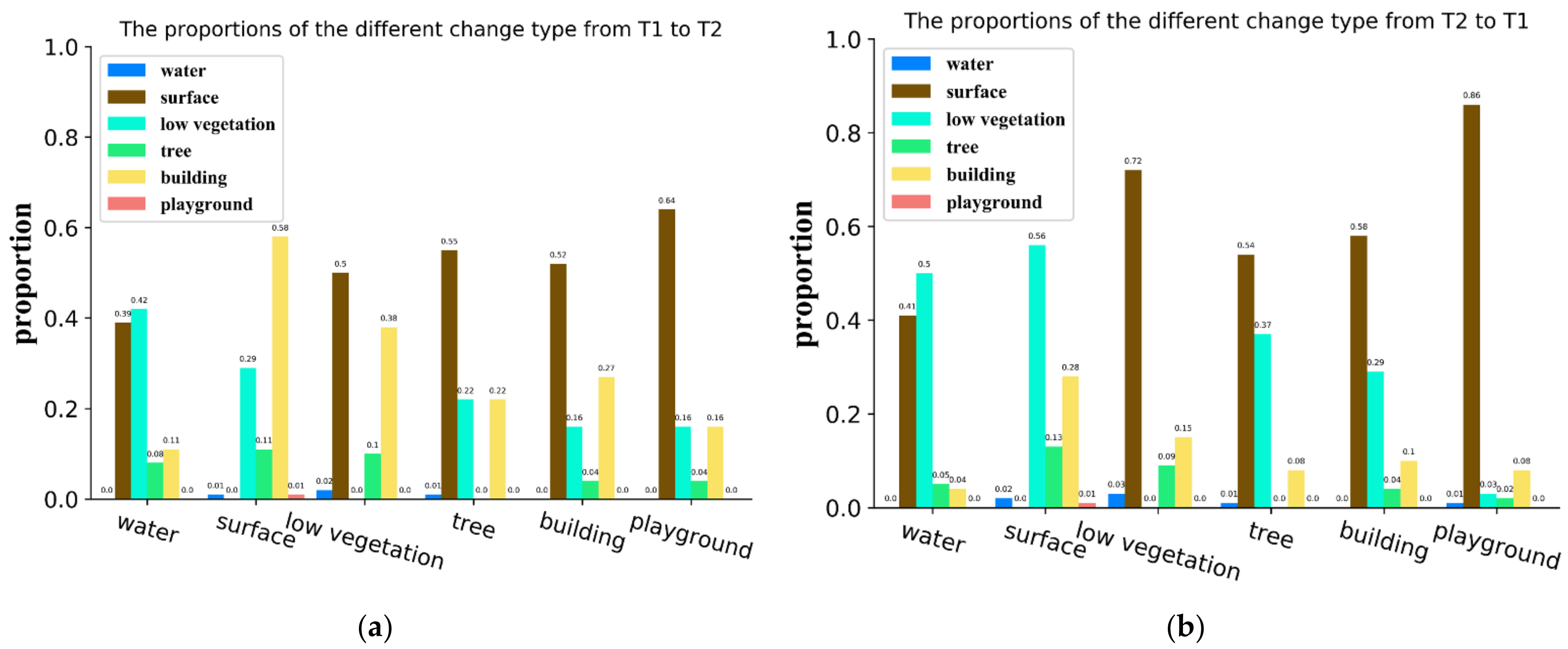
This paper contends that considering change relationships can enhance the performance of the semantic segmentation branch within post-classification methods. Land cover changes, unless triggered by abrupt natural events, follow certain patterns due to factors like urban planning. These patterns are defined as change relationships in this paper. We conducted a statistical analysis of different “from–to” change types based on the SECOND dataset [22], depicted in Figure 1, revealing inconsistent change-type probabilities and, consequently, change relationships among land cover classes. For instance, Figure 1a indicates that pixels classified as water in T1 (image taken at the 1st timestamp) transform to low vegetation (42%) more often than to trees (8%) in T2 (image taken at the 2nd timestamp). This underscores the value of the change relationship as an auxiliary predictor for land cover classes. Notably, the change relationship is bidirectional, as evident in Figure 1a,b. We interpret the change relationship from T1 to T2 as a probability distribution representing the shift from one land cover class to others. Conversely, the change relationship from T2 to T1 signifies the probability distribution of other land cover classes “transitioning into” a specific category. While temporal relationships have proven effective in multi-temporal image land cover class and video semantic segmentation [26,27,28,29], the method described earlier only considers one-way temporal relationships.

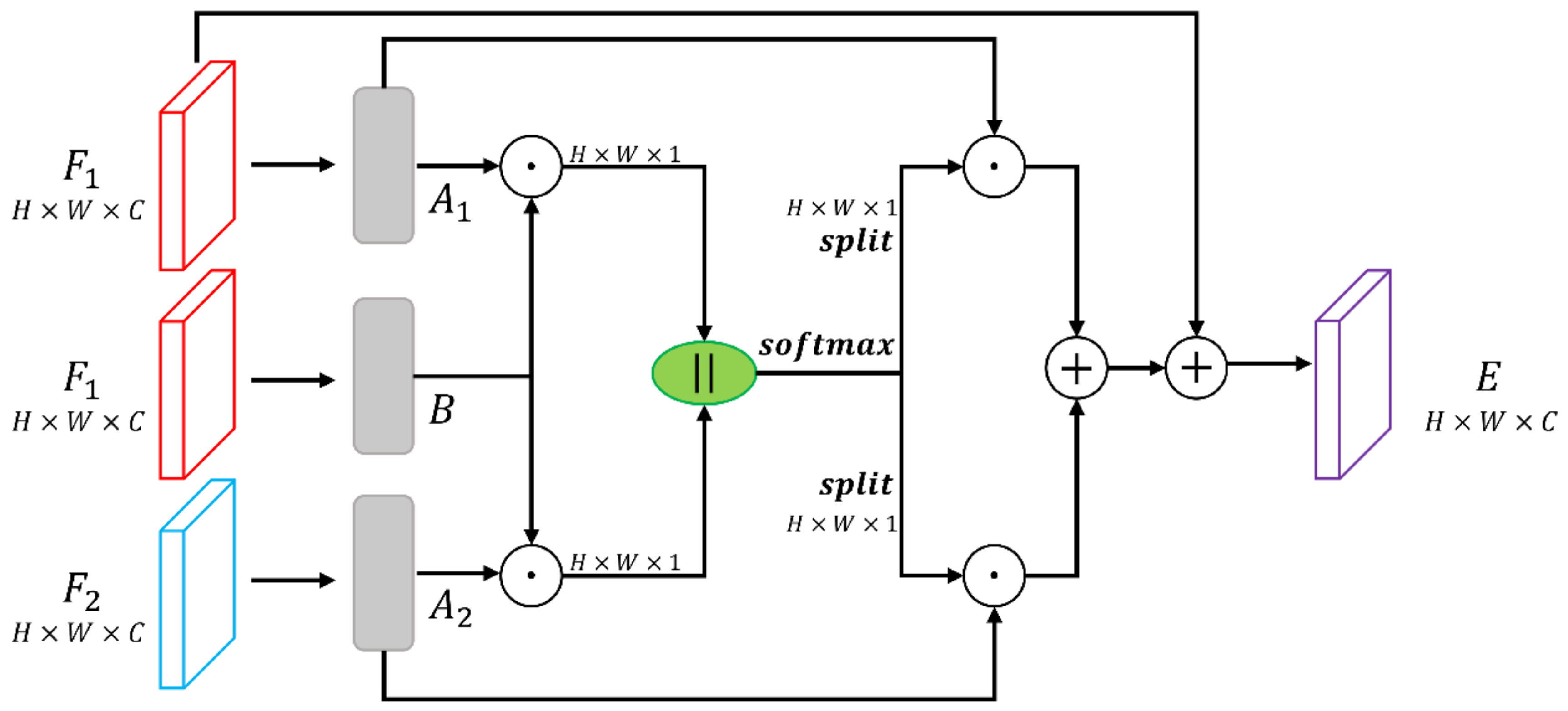
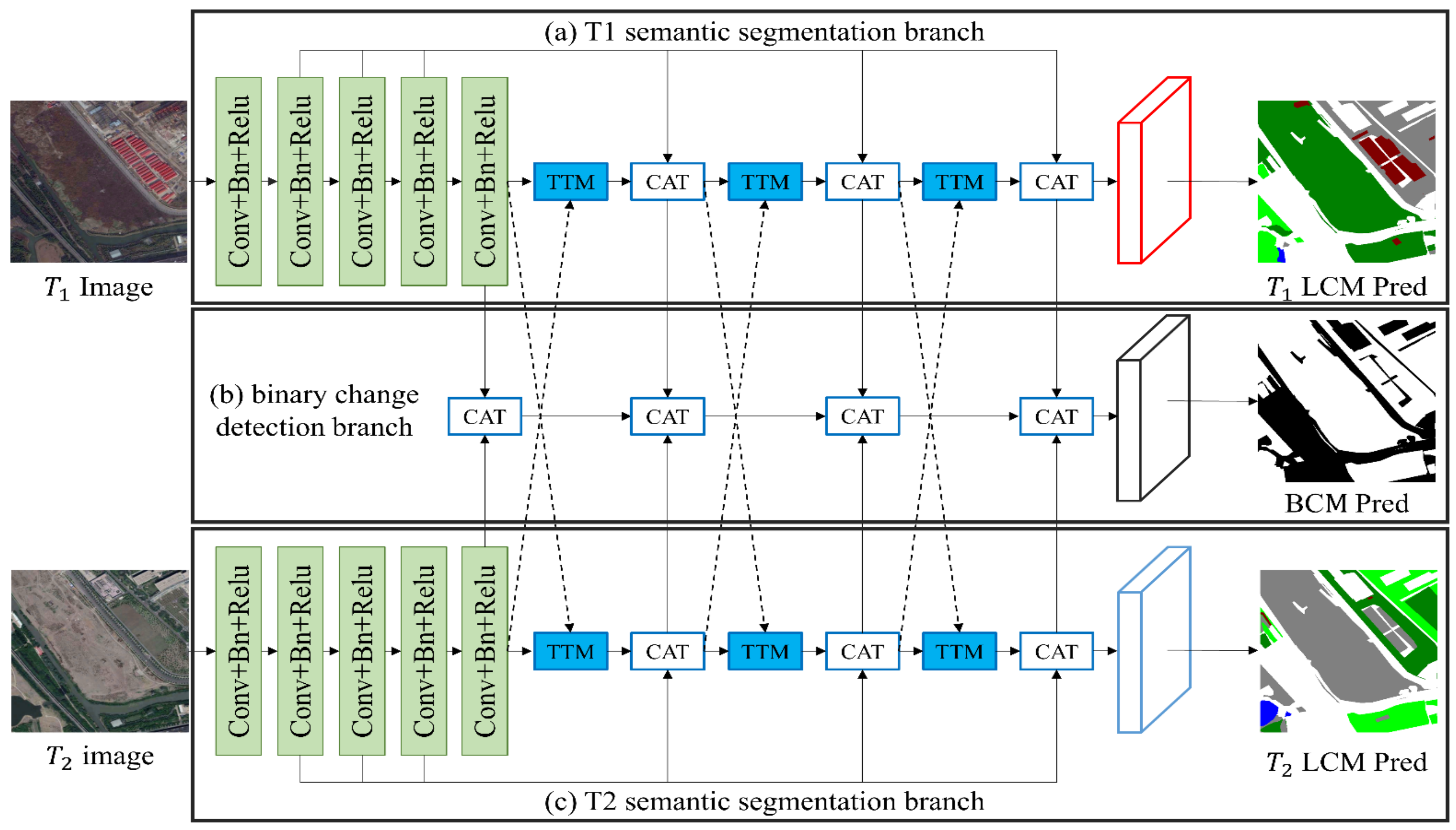
Building on the concept of change relationships in semantic change detection, we introduce the Temporal-Transform Module (TTM), inspired by spatial self-attention mechanisms [30,31,32]. TTM captures these relationships bidirectionally by evaluating feature similarities across temporal images. It enhances features in each temporal image by selectively integrating them with others, boosting mutual improvement. TTM can be seamlessly integrated into post-classification networks, enhancing performance without significant computational burden. Moreover, we present the Temporal-Transform Network (TTNet) founded on TTM for SCD, delineated in Figure 2. TTNet comprises three key components: two semantic segmentation branches (depicted in Figure 2a,c) and a binary change detection branch (Figure 2b). Each semantic segmentation branch, equipped with the feature pyramid decoder, incorporates three TTM layers to link the other semantic segmentation branch and capture bidirectional change relationships.

The contributions of this study are summarized as follows:

• We identify a two-way change relationship between “from-to” change types and analyze its significance in the semantic change detection task, deepening our comprehension of semantic change detection.
• Grounded in the concept of change relationships, we introduce the innovative Temporal-Transform Module to dynamically model these relationships, amplifying the discriminative capacity of feature maps.
• Integrating several TTMs into the semantic segmentation branch, augmented by the feature pyramid decoder, we devise a fresh Temporal-Transform Network for SCD. TTNet encompasses twin semantic segmentation branches and a binary change detection branch, predicting two land cover maps and a binary change map.
• Comprehensive experiments and analyses affirm the effectiveness of our approach, with comparisons showcasing TTNet’s superior performance on the SEONCD dataset in comparison to several benchmark methods.

2. Related Work

We categorize semantic change detection methods into two paradigms: the direct-classification method and the post-classification method. This section provides an overview of the relevant literature on these two approaches.

2.1. Direct-Classification Method

Direct-classification methods tackle semantic change detection by treating each detailed “from-to” change type as an independent class, and predict it with one or more classification strategies. In [33], a single input vector was formed by stacking bi-temporal remote sensing images. Subsequently, multi-class Support Vector Machines (SVMs) were employed for semantic change detection. Volpi et al. tried to incorporate both the stacked bi-temporal images and spatial context information into the SVM classifier [34], leading to improved performance. More recently, the integration of deep learning concepts into direct-classification methods has gained traction. In the realm of natural images, LambdaNet [35] was proposed to address multi-class directional change detection. LambdaNet employed a Siamese Convolutional Network to extract features from bi-temporal images, followed by feature concatenation and decoding to generate semantic change maps. A different approach was taken in [16], where bi-temporal street view images were mapped into two multi-scale feature spaces using a Siamese convolutional network. These feature maps were then up-sampled to the original image resolution, concatenated, and fed into a softmax classifier for semantic change map generation. To restore spatial detail in changed regions, Varghese et al. [16] and Prabhakar et al. [19] introduced UNet-like structures that employ skip-connections to fuse low-level and high-level features.

In remote sensing, Ref. [20] proposed a recurrent convolutional neural network (ReCNN) to learn combined spectral-spatial features. The ReCNN employed convolutional networks to transform bi-temporal images into high-level feature maps containing rich semantic information. These feature maps were then fed into a recurrent network to extract change information by modeling temporal dependencies. Moreover, unsupervised methods have also been applied to the direct-classification approach for semantic change detection, based on difference representation learning [36,37].

2.2. Post-Classification Method

In contrast to direct-classification methods, post-classification methods assume that each “from–to” change type is a combination of any two land-cover classes. Hence, these methods typically entail forecasting the two land-cover maps of bi-temporal images individually and subsequently identifying change regions. The final SCD outcomes arise from the multiplication of the binary change map and the two land-cover maps. Categorized by the manner of binary change map generation, post-classification methods can be grouped into two classifications: comparison methods and independence methods. Comparison methods predominantly hinge on the comparison of two land-cover maps to generate a binary change map. For instance, in [38], a convolutional neural network was initially deployed to generate urban distribution maps from bi-temporal Synthetic Aperture Radar (SAR) images. A subsequent mesh analysis was employed to derive an object-level semantic change map from these urban distribution maps. This straightforward approach has gained prominence as a benchmark for many semantic change detection tasks [25,39]. However, a notable drawback of comparison methods resides in the propensity for accumulating misclassification errors from land-cover maps, thereby leading to an increased occurrence of mis-detection in the resulting binary change map.

To address the issue of error accumulation, independent methods adopt the principle that predicting the binary change map should ideally remain unaffected by land-cover map considerations. In the work of [24], a model named HRSCD.str3 was introduced, incorporating two land-cover mapping branches and a binary change detection branch to jointly perform SCD. Here, the land-cover mapping branch network predicted the land-cover map for each temporal image using a Siamese Network framework. Simultaneously, pairs of images were processed through the binary change detection branch network to produce a binary change map. Seeking to enhance the accuracy of the binary change map by leveraging land-cover information, Ref. [24] extended this concept to HRSCD.str4. In HRSCD.str4, features extracted from the encoders of the two land-cover mapping branches were integrated into the binary change detection branch. Likewise, Ref. [22] introduced an Asymmetric Siamese Network (ASN) to extract feature pairs in an asymmetric manner.

3. Methodology

The architecture of the proposed TTNet is presented in Section 3.1. In Section 3.2, we provide the details of the key network module, i.e., the Temporal-Transform Module. Further elaboration on the utilized loss functions for model training is presented in Section 3.3.

3.1. Network Architecture

In this study, a Temporal-Transform Network is proposed for semantic change detection using bi-temporal remote sensing images. The overall architecture of TTNet is depicted in Figure 2, comprising three components: two semantic segmentation branches (Figure 2a,c) and a binary change detection branch (Figure 2b). Taking a pair of bi-temporal remote sensing images as input, the semantic segmentation branches generate two land cover maps (LCMs) for the respective bi-temporal images. Subsequently, the feature maps extracted from the semantic segmentation branches are fed into the binary change detection branch to generate a binary change map (BCM). Finally, the BCM is multiplied individually with the two LCMs to derive two semantic change maps.

3.1.1. Semantic Segmentation Branch

As depicted in Figure 2, we employ a Siamese convolutional neural network with shared weights for semantic segmentation. The structure of the semantic segmentation branch follows an encoder–decoder framework. The encoder comprises a bottom-up pathway designed to extract features, where our encoder backbone utilizes a pre-trained ResNet34 [40] from ImageNet. Given a high-resolution remote sensing image $I_t\in R^{H\times W\times 3}$ as the input, with H and W denoting height and width, respectively, a set of multi-scale feature maps ${\left\{F_l^t\in R^{\frac{H}{2^{l+1}}\times \frac{W}{2^{l+1}}\times C_l}\right\}}_{l=\mathrm{1,2},\mathrm{3,4}}$ are extracted through the encoder. Here, $t$ corresponds to the temporal dimension, and $C_l$ signifies the channel number of the $l_{th}$ layer feature map.

In the decoder, which involves a top-down pathway for upsampling, feature maps are transformed to ${\left\{{\overline{F}}_l^t\in R^{\frac{H}{2^{l+1}}\times \frac{W}{2^{l+1}}\times C_l}\right\}}_{l=\mathrm{4,3},\mathrm{2,1}}$ using skip connections to amalgamate multi-scale features from the encoder. As emphasized in Section 1, the utilization of the change relationship can enhance the semantic segmentation branch’s performance. Consequently, within the decoder, we initially incorporate a Temporal-Transform Module to capture the change relationship between $T_1$ feature maps $F_4^1$ and $T_2$ feature maps $F_4^2$. Subsequently, the TTM is sequentially cascaded three times to refine the feature representation and restore the feature map resolution to ($\frac{H}{4},\frac{W}{4}$). Ultimately, the resulting feature map ${\overline{F}}_1^t\in R^{\frac{H}{4}\times \frac{W}{4}\times C_1}$ is passed through a $1\times 1$ convolution layer to generate the land cover map. Detailed information regarding the TTM is elaborated in Section 3.2.

3.1.2. Binary Change Detection Branch

Differing from the binary change detection branch present in the prevailing SCD methods [22,24], we depart from the use of an additional encoder module to capture features from both changed and unchanged areas. Instead, we directly harness the features derived from the semantic segmentation branches to yield the difference features. Given that the land cover map labels have more abundant semantic category information compared to the binary change map label, concatenating the feature maps from the two semantic segmentation branches to generate the difference feature maps facilitates a clearer distinction between changed and unchanged regions. Meanwhile, removing the feature encoder in the binary change detection branch simplifies the network parameters and reduces computational load without sacrificing performance.

As there is no need for an encoder, the binary change detection branch exclusively integrates a decoder. Analogous to the semantic segmentation branch, the decoder employs skip-connection operations to restore boundary information within the changed area. Commencing with the top-level feature maps $F_4^1$ and $F_4^2$ from the two semantic segmentation branches, we concatenate these as the initial input $F_4^d$ for the decoder. Subsequently, this initial input is subjected to a 2× upsample via standard bilinear interpolation and then combined with the low-level difference feature maps $F_3^d$, obtained by concatenating ${\overline{F}}_3^1$ and ${\overline{F}}_3^2$. After two iterations of this process, a classifier incorporating a $1\times 1$ convolution layer and a 4× bilinear upsampling layer is employed to predict the binary change map.

3.2. Temporal-Transform Module (TTM)

3.2.1. Design Motivation

The current approach in semantic change detection involves the prediction of distinct land cover maps and a binary change map using bi-temporal images. As highlighted in Section 1, past research has ignored the significance of the change relationship within land cover classification. Consequently, the primary objective of this research is to grasp the change relationship’s importance and enhance the performance of the semantic segmentation branch. Guided by the notion of the change relationship, our focus shifts to the impact of feature information from one image on another. This naturally directs us toward the spatial attention mechanism. Traditionally utilized in semantic segmentation tasks, the spatial attention mechanism serves to comprehend the interdependence of feature maps’ positions within the spatial dimension. Drawing inspiration from this spatial attention mechanism, we capture the change relationship through evaluating the similarity between feature maps of bi-temporal images across the temporal dimension.

3.2.2. Module Details

The structure of the Temporal-Transform Module can be observed in Figure 3. To elaborate on the influence of the T2 image on the T1 image, let us consider two equi-dimensional feature maps: $F_1\in R^{C\times H\times W}$ and $F_2\in R^{C\times H\times W}$, which are extracted from the bi-temporal images. Feeding $F_1$ into a $1\times 1$ convolutional layer results in two novel feature maps, $A_1$ and $\mathrm{B}$, both belonging to $R^{K\times H\times W}$. Meanwhile, applying feature map $F_2$ to a $1\times 1$ convolutional layer produces a new feature map, $A_2$, within $R^{K\times H\times W}$. The probability map representing the change relationship, denoted as $S$ and within $R^{2\times H\times W}$, can be computed as follows:

$$S_t^i=\frac{exp\left(A_t^i\cdot B^i\right)}{{\sum }_{t=1}^{N=2}exp\left(A_t^i\cdot B^i\right)}$$

(1)

where $S_t^i$ signifies the influence of feature $F_t$ on feature $F_1$ at position $i$. When the feature representations of the bi-temporal images mutually affect each other at position $p$, it enhances the correlation between them. Subsequently, we conduct an element-wise multiplication for the input features $F_t$ and $F_t$ to selectively retain information. Ultimately, we employ an element-wise summation to aggregate the features of bi-temporal images and yield the ultimate output $E\in R^{C\times H\times W}$ as follows:

$$E^i={\sum }_{t=1}^{N=2}(S_t^i{A}_t^i)+F_1$$

(2)

where $E^i$ represents the weighted summation of features at position $i$. Hence, the final output map $E$ encapsulates the bi-temporal image information acquired through the TTM.

3.3. Loss Function

We utilize the binary cross-entropy loss function to optimize the binary change detection branch and the cross-entropy loss function to optimize the semantic segmentation branch.

The binary cross-entropy loss is defined as follows:

$${\mathcal{L}}_{BCE}=-\frac{1}{N}\sum _{i=1}^N\left(y_i\log \left({\widehat{y}}_i\right)+\left(1-y_i\right)\log \left(1-{\widehat{y}}_i\right)\right)$$

(3)

where $y_i\in \left\{0, 1\right\}$ represents the ground truth label (1 for the changed class and 0 for the unchanged class). ${\widehat{y}}_i\in \left[0,1\right]$ indicates the predicted probability of the $i_{t\mathrm{h}}$ pixel belonging to the changed class. $N$ denotes the total number of pixels in the ground truth label.

The cross-entropy loss for the semantic segmentation branch is defined as follows:

$${\mathcal{L}}_{CE}=-\frac{1}{N\times T}\sum _{t=1}^T\sum _{i=1}^N\sum _{c=1}^C{y}_{tic}\log {\widehat{y}}_{tic}$$

(4)

where $C$ denotes the number of land cover classes, and $T$ represents the number of temporal dimensions. $y_{ic}\in \left\{0, 1\right\}$ stands for the ground truth label, while ${\widehat{y}}_{ic}\in \left[0,1\right]$ represents the predicted probability of the $i_{t\mathrm{h}}$ pixel belonging to the $c_{t\mathrm{h}}$ class.

The final loss function used to end-to-end train TTNet is defined as

$$\mathcal{L}={\lambda }_1{\mathcal{L}}_{BCE}+{\lambda }_2{\mathcal{L}}_{CE}$$

(5)

where ${\lambda }_1$ and ${\lambda }_2$ represent the loss weights for balancing ${\mathcal{L}}_{BCE}$ and ${\mathcal{L}}_{CE}$, respectively. They are both set to 1 in this study.

4. Experiment and Analysis

4.1. Dataset and Metric

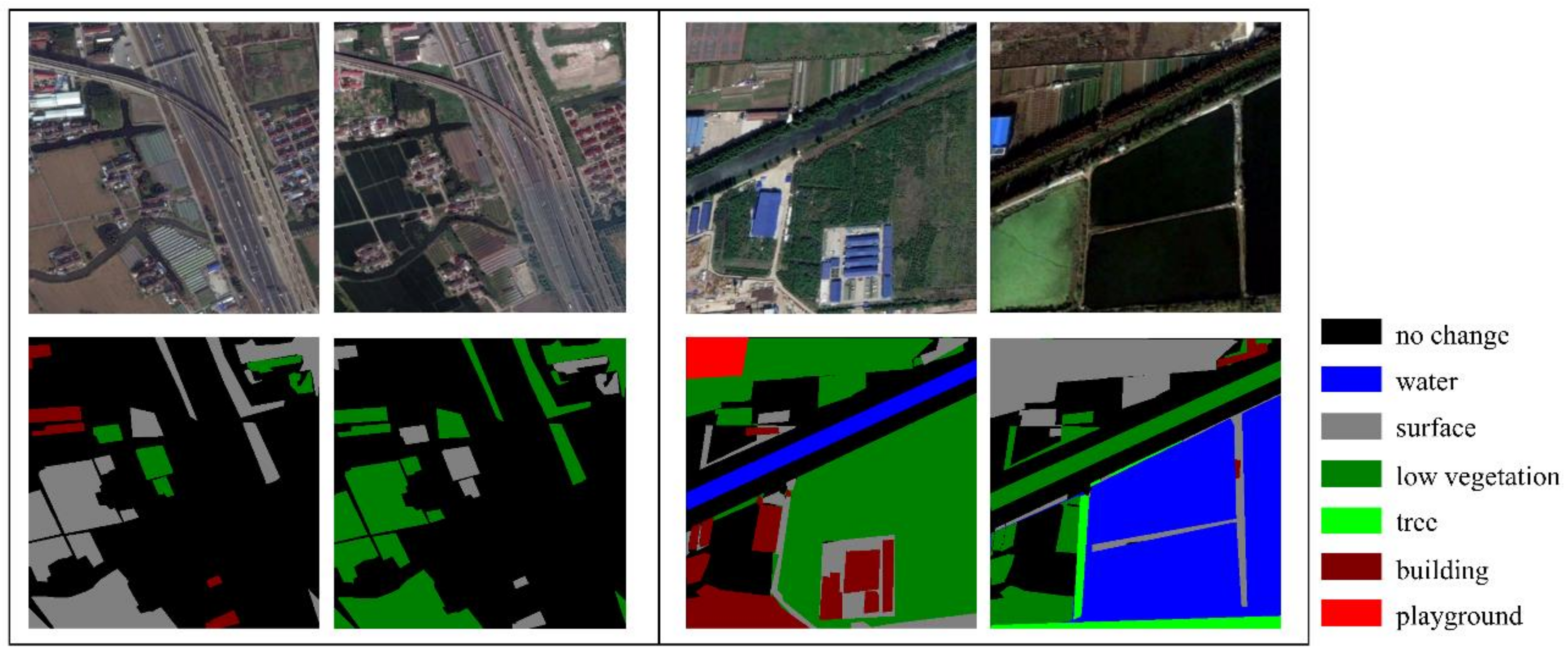
The benchmark dataset chosen for our experiments is the SECOND dataset [22]. Figure 4 presents several samples from the SECOND dataset. This dataset encompasses 4662 pairs of aerial images with spatial resolutions varying from 0.5 m to 3 m. It is further divided into training and testing subsets, with 2968 pairs allocated for training and 1694 pairs for testing. Each sample comprises two images from distinct time phases and corresponding land cover classification labels. Each image is sized at 512 × 512 pixels, with pixel-wise annotations belonging to one of the 7 classes (no change, water, surface, low vegetation, tree, building, and playground). Considering that only 2968 sample pairs from the SECOND dataset were available for training, we allocated 2000 and 968 sample pairs for training and testing, respectively. To gauge performance, we employed the mean Intersection over Union (mIoU) metric.

4.2. Implementation Details

Our method and benchmark methods were implemented using the PyTorch framework. We employed the Adam optimizer with a batch size of 8 for network optimization over 80 epochs. The initial learning rate was set to ${1\times 10}^{-4}$ and was adjusted to ${1\times 10}^{-5}$ after 50 epochs. Data augmentation techniques included random horizontal and vertical flips, scaling between 1 and 2, and random rotations at 0, 90, 180, and 270 degrees. All experiments were conducted on a single Tesla P40 GPU under consistent settings. The TTM utilized 1 × 1 convolutional layers with 256 output channels.

4.3. Benchmark Methods

To assess the effectiveness of our proposed method, we conducted a comprehensive comparison with six prominent benchmark methods designed for semantic change detection. These methods include:

• HRSCD.str1 [24]: This method employs a direct comparison strategy for land cover maps. It trains a network to generate the LCMs of bi-temporal images and then compares these maps pixel by pixel to derive the semantic change maps.
• HRSCD.str2 [24]: This approach adopts a direct semantic change detection strategy, treating each change type as a distinct and independent class. For instance, a pixel transitioning from water to surface is labeled as class A. This transforms the SCD problem into a semantic segmentation task.
• HRSCD.str3 [24]: Using a different approach, this method predicts the LCMs and the BCM separately. It employs two semantic segmentation branches to predict the LCMs of the bi-temporal images, while the binary change detection branch predicts the BCM.
• HRSCD.str4 [24]: Similar in architecture to HRSCD.str3, this method differentiates itself by fusing features from the encoder of the semantic segmentation branches during the BCM prediction.
• Deeplab v3+ [41]: This approach replaces the semantic segmentation branch of HRSCD.str4 with Deeplab v3+, a model utilizing an Atrous Spatial Pyramid Pooling (ASPP) module with different rates to capture spatial contextual information.
• PSPNet [42]: In this method, the semantic segmentation branch of HRSCD.str4 is substituted with PSPNet. PSPNet employs a multi-scale pyramid pooling module (PPM) to capture scene context in the spatial dimension.

4.4. Comparison with Benchmark Methods

In our comparison with benchmark methods, we present results for both semantic change detection and semantic segmentation. The semantic change detection results are obtained using the predicted binary change map from the binary change detection branch, allowing for an evaluation of the overall method performance. Moreover, to specifically showcase the effectiveness of the Temporal-Transform Module in enhancing the semantic segmentation branch, we also present semantic segmentation results based on labeled binary change maps. This approach eliminates the influence of the binary change detection branch.

4.4.1. Assessment of Semantic Change Detection

Quantitative Analysis:

Table 1. The quantitative results for semantic change detection achieved by TTNet and six benchmark methods on the SECOND dataset. The best values are marked in bold.

Method	Backbone	mIoU(%)	No Change	Water	Surface	Low Vegetation	Tree	Building	Playground
HRSCD.str1	ResNet34	29.75	62.15	18.42	26.53	24.67	14.36	33.23	28.87
HRSCD.str2	ResNet34	33.20	85.73	0.00	32.78	28.53	7.00	47.00	30.59
HRSCD.str3	ResNet34	35.30	84.47	17.11	30.18	30.12	16.70	43.07	25.44
HRSCD.str4	ResNet34	43.45	87.20	23.42	39.18	34.51	21.50	55.15	43.19
Deeplab v3+	ResNet34	42.98	87.01	23.55	37.91	33.40	20.60	55.01	43.40
PSPNet	ResNet34	44.36	87.01	25.96	39.92	34.33	22.77	56.04	44.48
TTNet	ResNet34	45.91	87.18	29.59	40.82	35.11	22.81	56.26	49.61

showcases the quantitative outcomes of semantic change detection for TTNet in comparison with six benchmark methods on the SECOND dataset. The optimal performance is highlighted in bold. From the table, it is evident that TTNet achieves the highest performance in terms of mIoU and per-class semantic IoU, excluding the “no change” class. HRSCD.str1, HRSCD.str2, and HRSCD.str3 exhibit the lowest mIoU, all falling below 40%. By incorporating land cover label information into the binary change detection branch, HRSCD.str4 achieves a notable mIoU of 43.45%, marking an 8.15% improvement. In contrast, PSPNet, which emphasizes capturing spatial context, marginally improves mIoU by 0.91%, while Deeplab v3+ slightly reduces mIoU by 0.47%. This indicates that the stability of capturing spatial context for SCD is uncertain. In stark comparison, TTNet, which focuses on capturing change relationships, enhances mIoU by 2.46% compared to HRSCD.str4. These quantitative results underscore the remarkable performance of TTNet in semantic change detection.

4.4.2. Assessment of Semantic Segmentation

To provide further insight into TTNet’s superior performance, we initially present the outcomes of binary change detection in

Table 2. The quantitative results for the binary change detection branch, comparing TTNet with five benchmark methods. The best values are marked in bold.

Method	mIoU(%)	No Change	Change
HRSCD.str1	48.31	62.15	34.47
HRSCD.str3	63.59	84.47	42.71
HRSCD.str4	70.28	87.20	53.36
Deeplab v3+	70.13	87.01	53.25
PSPNet	70.49	87.01	53.97
TTNet	70.51	87.11	53.91

. Subsequently, we present the quantitative results for semantic segmentation obtained by multiplying the predicted land cover maps with the labeled binary change map, as showcased in

Table 3. The semantic segmentation quantitative results of TTNet and five benchmark methods on the SECOND dataset. The best values are marked in bold.

Method	Backbone	mIoU(%)	No Change	Water	Surface	Low Vegetation	Tree	Building	Playground
HRSCD.str1	ResNet34	60.95	100.00	38.06	61.37	50.22	45.98	76.47	54.58
HRSCD.str3	ResNet34	61.44	100.00	39.34	61.41	51.65	45.95	76.33	55.42
HRSCD.str4	ResNet34	61.46	100.00	39.17	62.06	52.35	45.19	77.44	56.12
Deeplab v3+	ResNet34	60.02	100.00	38.30	60.32	50.93	42.55	76.42	52.02
PSPNet	ResNet34	62.18	100.00	41.13	62.83	52.39	46.58	77.39	54.95
TTNet	ResNet34	65.36	100.00	45.76	67.99	56.77	48.24	79.71	59.08

. It is important to note that HRSCD.str2, due to its direct-classification method, is excluded from Table 2 and Table 3.

Quantitative Analysis: Analyzing the initial three rows of Table 3, we observe that HRSCD.str1 and HRSCD.str3 yield similar semantic segmentation outcomes as HRSCD.str4. While, referring to Table 2, it becomes evident that HRSCD.str4 attains a significantly improved mIoU of 70.28%, marking an enhancement of 21.97% and 6.69% over HRSCD.str1 and HRSCD.str3 in terms of binary change detection outcomes, respectively. This highlights that the integration of semantic segmentation branch features into the binary change detection branch notably enhances binary change map predictions.

In the last four rows of Table 2, the binary change detection branch displays a fairly consistent performance among the four methods, with TTNet achieving the highest mIoU of 70.51% and the lowest being 70.13% (a gap of 0.38%). Conversely, it is worth noting that the performance variations within the semantic segmentation branch among these methods become evident when referring to Table 3. When compared to HRSCD.str4 and PSPNet, TTNet stands out by enhancing the mIoU from 61.46% and 62.18% to 65.36%. This contrast in semantic mIoU significantly widens to 5.34% when compared to Deeplab v3+.

These outcomes indicate that TTNet’s enhanced performance in semantic change detection arises from its improved semantic segmentation accuracy. This is primarily attributed to TTNet’s utilization of TTM to comprehend the change relationships within bi-temporal images. This understanding of change relationships assists the model in identifying altered regions and characterizing their change types, thereby mitigating issues of un-detection and mis-detection.

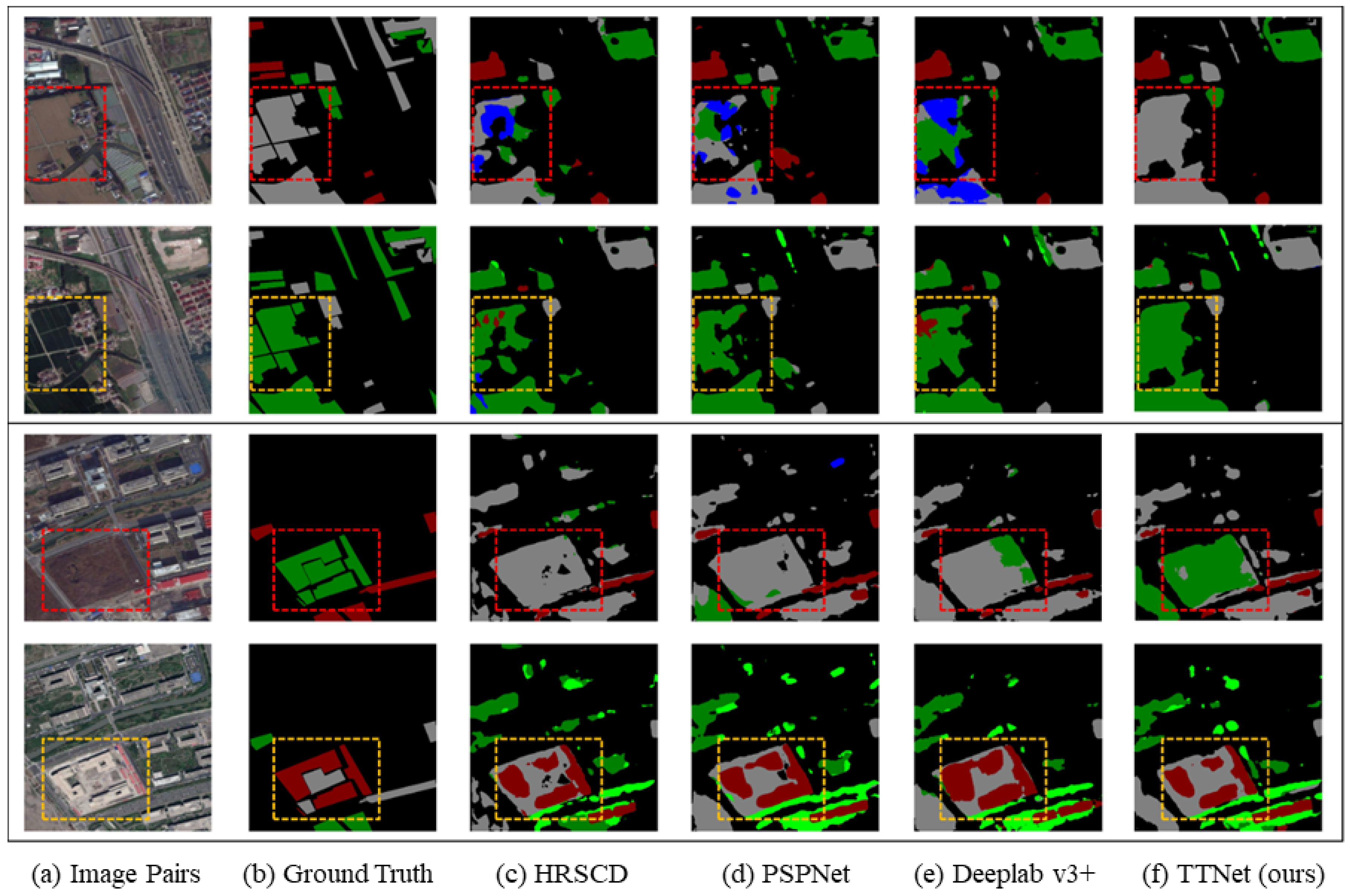
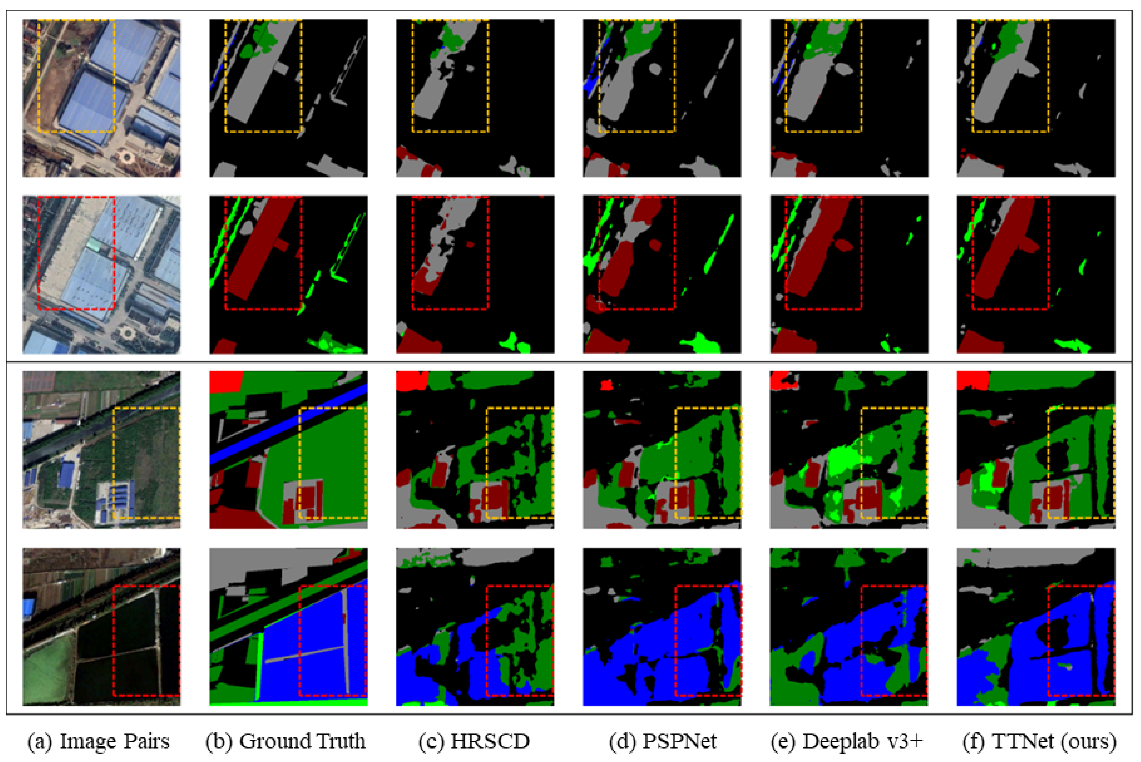
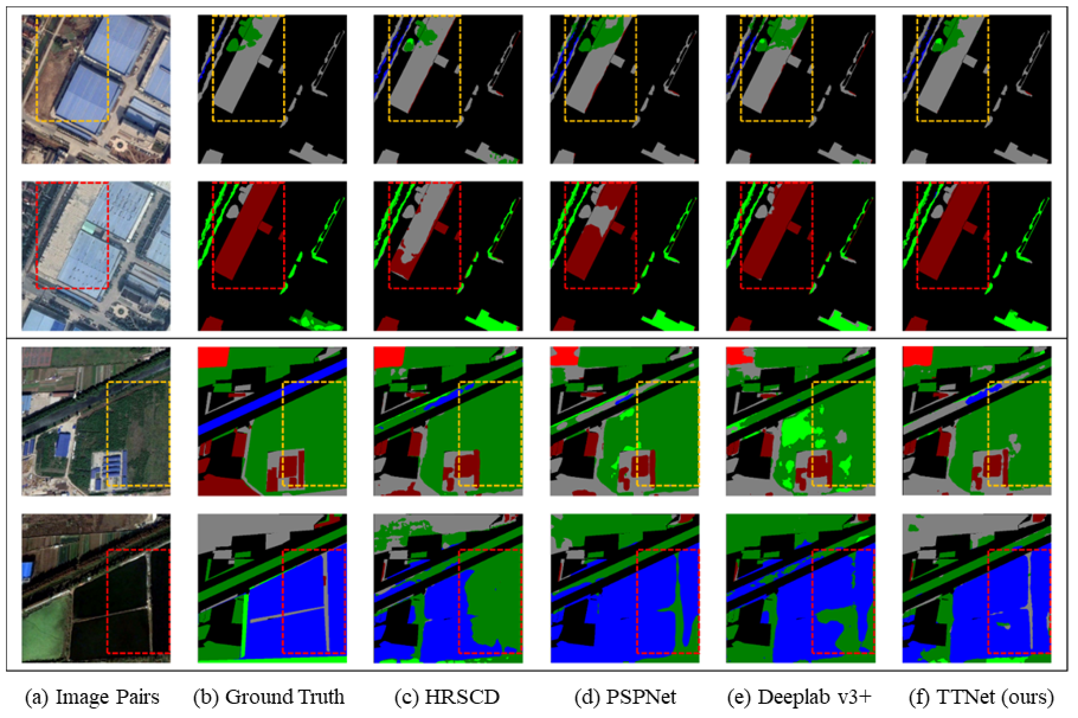
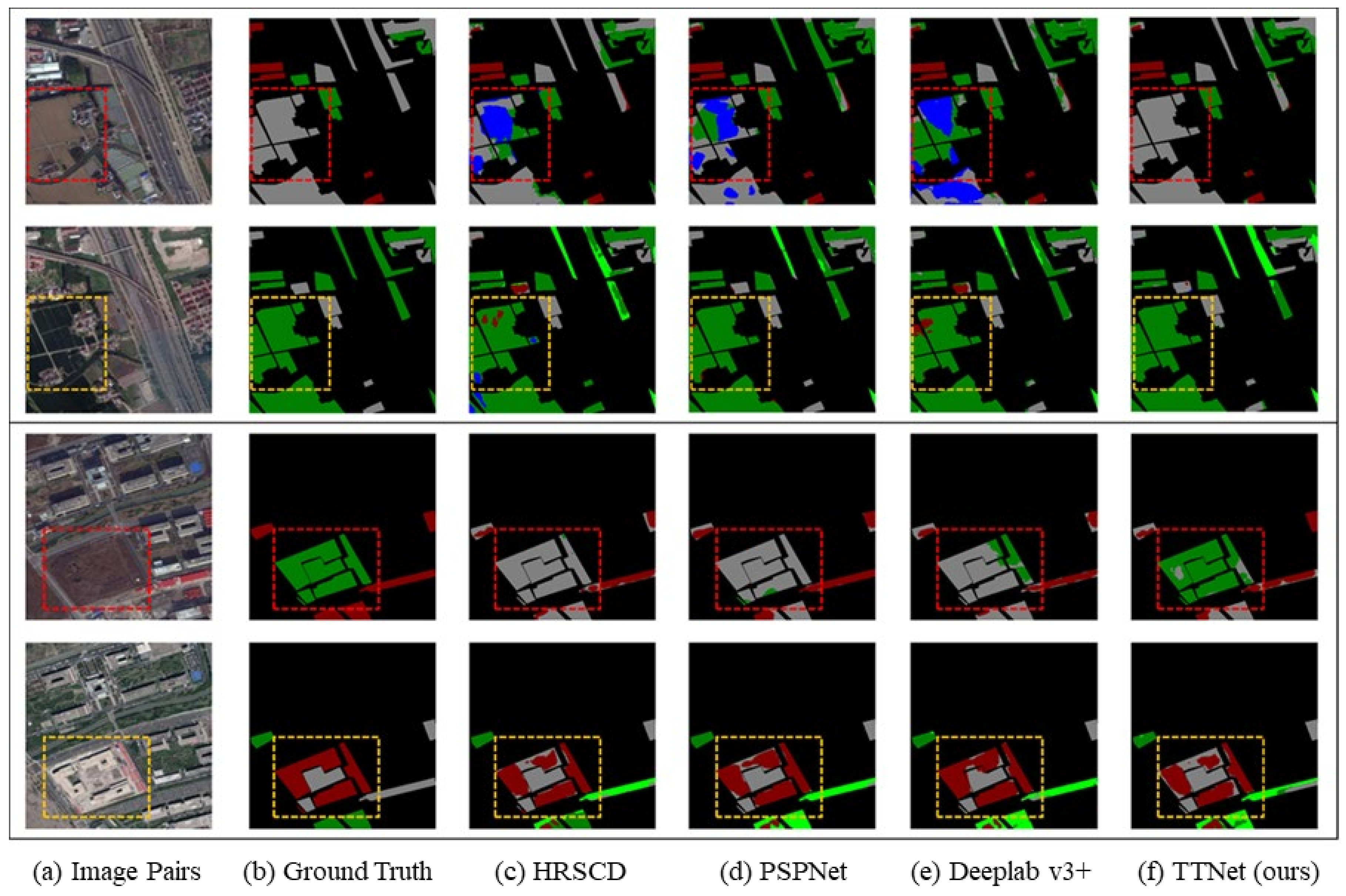
4.4.3. Visualization Comparison

Figure 5 and Figure 6 offer a visual comparison of the un-detection and mis-detection problems, respectively, based on the predicted binary change map. Meanwhile, Figure 7 and Figure 8 provide visualization comparison results based on the labeled binary change map. Across all these visualizations, it is evident that the proposed TTNet outperforms the six benchmark methods.

In Figure 5 and Figure 7, the benchmark methods exhibit significant un-detection issues, particularly in cases where the spectral features of change regions bear resemblance. Notably, HRSCD.str4 exhibits shortcomings in identifying certain conspicuous change types, such as the “surface-to-building” change and “low vegetation-to-water” transition. Even with spatial context information capture, PSPNet and Deeplab v3+ still struggle with un-detection problems. In contrast, TTNet significantly mitigates un-detection problems even when dealing with similar spectral features in bi-temporal images.

Moreover, all benchmark methods encounter mis-detection problems when the spectral features of change regions diverge. As observed in Figure 6 and Figure 8, HRSCD.str4 inaccurately predicts surface as water or vegetation. This misclassification is more pronounced in PSPNet and Deeplab v3+, suggesting that context information might introduce noise in bi-temporal semantic segmentation. TTNet effectively curbs the influence of noise by learning the change relationship between bi-temporal images, accurately determining the current land cover class of change regions.

4.5. Ablation Study

To comprehensively analyze and discuss the performance of our proposed method, with a specific emphasis on exploring why certain TTM configurations outperform others, we have conducted several ablation studies. These studies are designed to delve into critical aspects such as the insertion positions, architectural design, and weight-sharing mechanisms of the TTM, aiming to analyze the rationale behind TTM configurations and their strategic placement within the model architecture.

4.5.1. Positions for TTM Insertion

To assess the impact of inserting the TTM at different layers, we experiment with placing the TTM at various stages within the decoder of the semantic segmentation branch. We conduct comparisons across seven different network configurations: TTNet.baseline, TTNet.TTM2, TTNet.TTM3, TTNet.TTM4, TTNet.TTM42, TTNet.TTM43, and TTNet.TTM432. Similar to Section 4.4, we present the results of this ablation study for different TTM insertion positions, considering both the predicted and labeled binary change maps. These results are detailed in

Table 4. Ablation study on different TTM insertion positions based on predicted binary change map. The “√” symbol denotes the insertion of TTM at the current layer. The best values for TTNet and HRSCD.str4 are marked in bold.

Method	${\mathit{F}}_4$	${\mathit{F}}_3$	${\mathit{F}}_2$	mIoU(%)	$∆\mathbf{a}$(%)
TTNet.baseline				44.43	-
TTNet.TTM2			√	44.41	−0.02
TTNet.TTM3		√		44.40	−0.03
TTNet.TTM4	√			44.85	0.42
TTNet.TTM42	√		√	44.79	0.36
TTNet.TTM43	√	√		44.97	0.54
TTNet.TTM432	√	√	√	45.91	1.48
HRSCD.str4				43.45	-
HRSCD.str4.TTM432	√	√	√	44.76	1.31

and

Table 5. Ablation study on different TTM insertion positions based on labeled binary change map. The “√” symbol denotes the insertion of TTM at the current layer. The best values for TTNet and HRSCD.str4 are marked in bold.

Method	${\mathit{F}}_4$	${\mathit{F}}_3$	${\mathit{F}}_2$	mIoU(%)	$∆\mathbf{a}$(%)
TTNet.baseline				62.28	-
TTNet.TTM2			√	61.55	−0.73
TTNet.TTM3		√		61.61	−0.67
TTNet.TTM4	√			63.58	1.30
TTNet.TTM42	√		√	64.66	2.38
TTNet.TTM43	√	√		64.70	2.41
TTNet.TTM432	√	√	√	65.36	3.08
HRSCD.str4				61.76	-
HRSCD.str4.TTM432	√	√	√	65.17	3.41

, which evaluate the performance of both semantic change detection and semantic segmentation, respectively.

Starting with the overall performance of semantic change detection, the results in Table 4 show that TTNet.baseline attains a 44.43% mIoU. Then, we progressively incorporate the TTM along the decoder’s top-down pathway after $F_4,{ F}_3$, and $F_2$. It can be observed that TTNet.TTM4 and TTNet.TTM43 achieve 44.85% mIoU and 44.97% mIoU, respectively, thus enhancing TTNet.baseline by 0.42% and 0.54%. By introducing TTM across all feature layers, TTNet.TTM432 achieves the most favorable outcome at 45.91%, elevating TTNet.baseline by 1.48%. Furthermore, applying TTM to HRSCD.str4 increases mIoU to 44.76, resulting in a 1.31% enhancement over the basic HRSCD.str4.

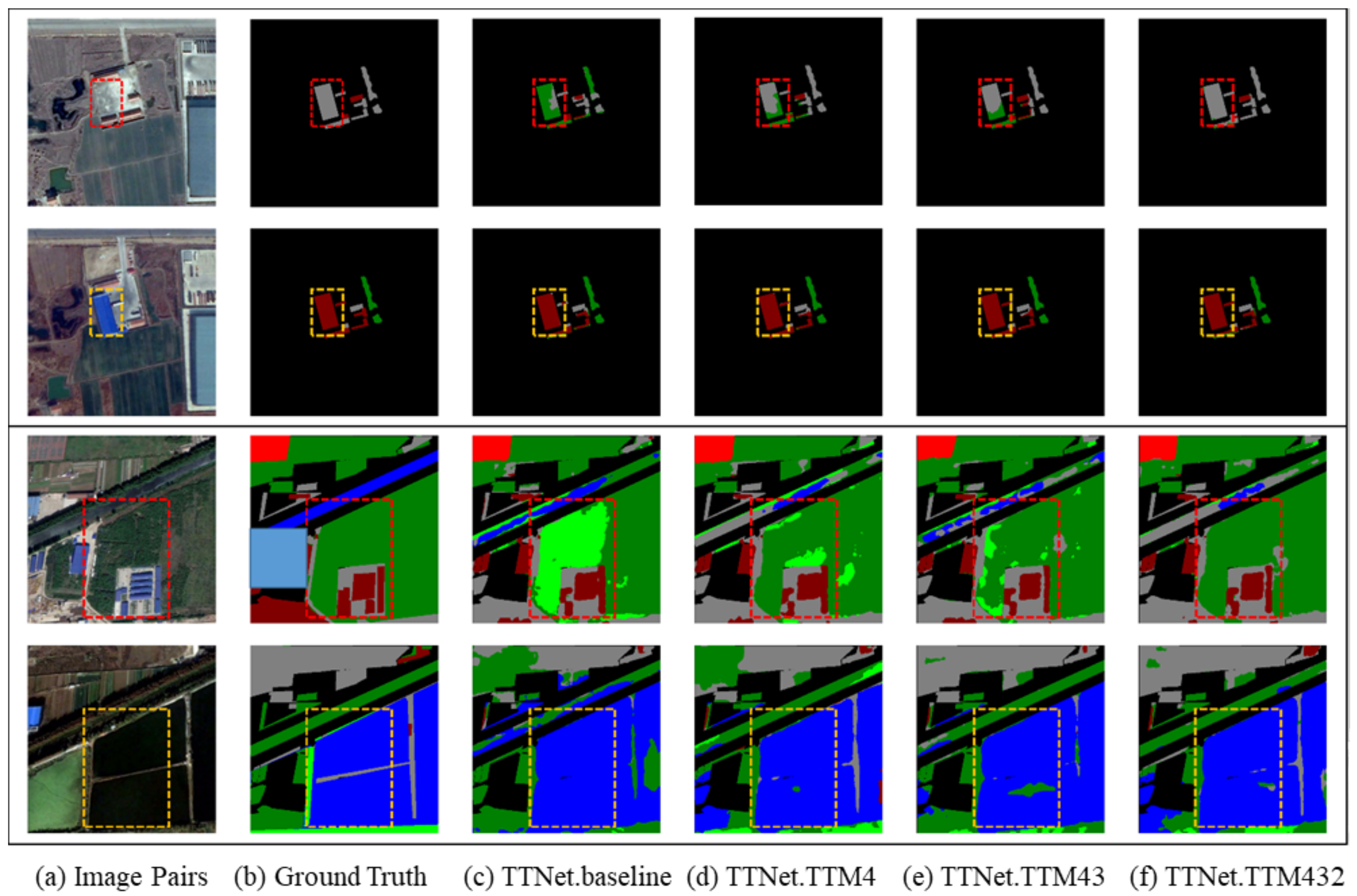
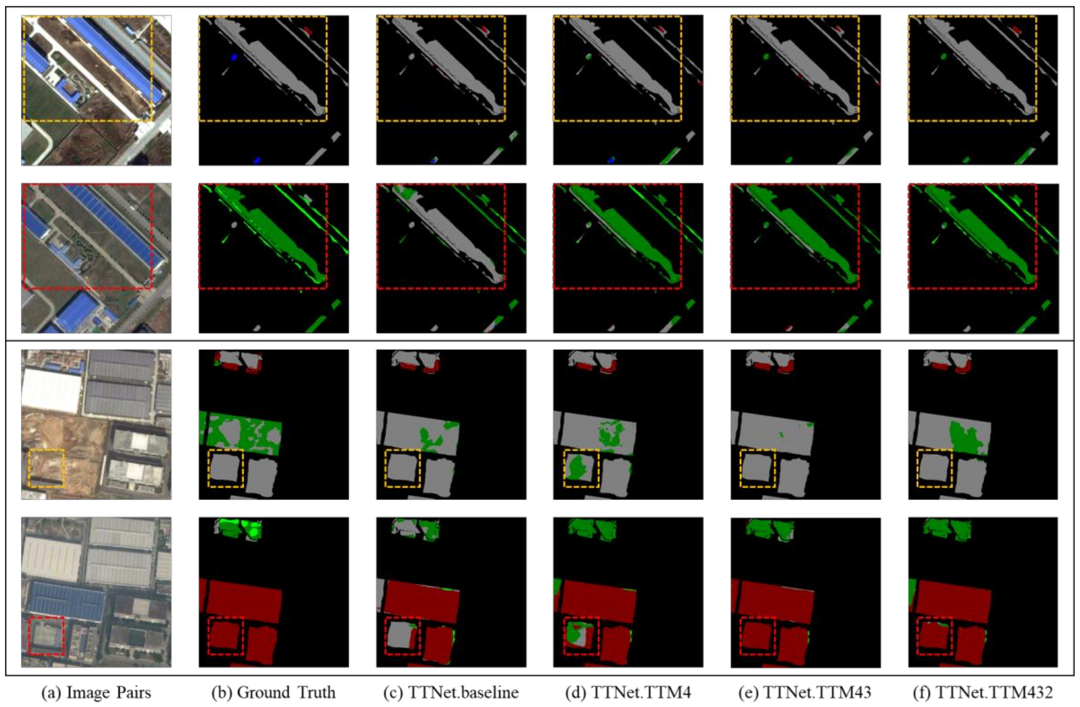
Next, we explore TTM’s impact on the performance of the semantic segmentation branch. As detailed in Table 5, TTNet.TTM432 outperforms all other network configurations, showcasing a remarkable 65.36% mIoU and a significant 3.08% enhancement over TTNet.baseline. Notably, TTNet.TTM42 and TTNet.TTM43 also contribute improvements of 2.38% and 2.41%, respectively. Similarly, the inclusion of TTM in HRSCD.str4 leads to a 3.41% enhancement in mIoU. This observation is further supported by the visual comparison examples presented in Figure 9 and Figure 10, where TTNet.TTM432 effectively mitigates issues of un-detection and mis-detection.

In summary, the consistent improvement trend observed in both label-based and prediction-based experimental results, as depicted in Table 4 and Table 5, underlines TTM’s capacity to achieve enhanced outcomes by capturing change relationships and displaying robust generalization performance.

Furthermore, the above ablation studies show that the TTNet.TTM 432 configuration outperforms others. As shown in Table 4 and Table 5, inserting TTM only after $F_2$ or $F_3$ yields negative impacts. This phenomenon can likely be attributed to the absence of comprehensive guidance from high-level semantic information. $F_4$, with its broader receptive field and richer semantic features, appears to play a pivotal role. Skipping $F_4$ and directly placing TTM after $F_2$ or $F_3$ might introduce noise due to the lack of substantial semantic context in the corresponding phase’s features. Consequently, this could lead to a degradation in TTM’s performance. This interpretation gains further substantiation from the observations in rows 5 and 6 of both Table 4 and Table 5. The noticeable improvements in TTNet.TTM42 and TTNet.TTM43 upon inserting TTM after $F_4$ underscore the irreplaceable role of high-level semantic information in effectively capturing change relationships.

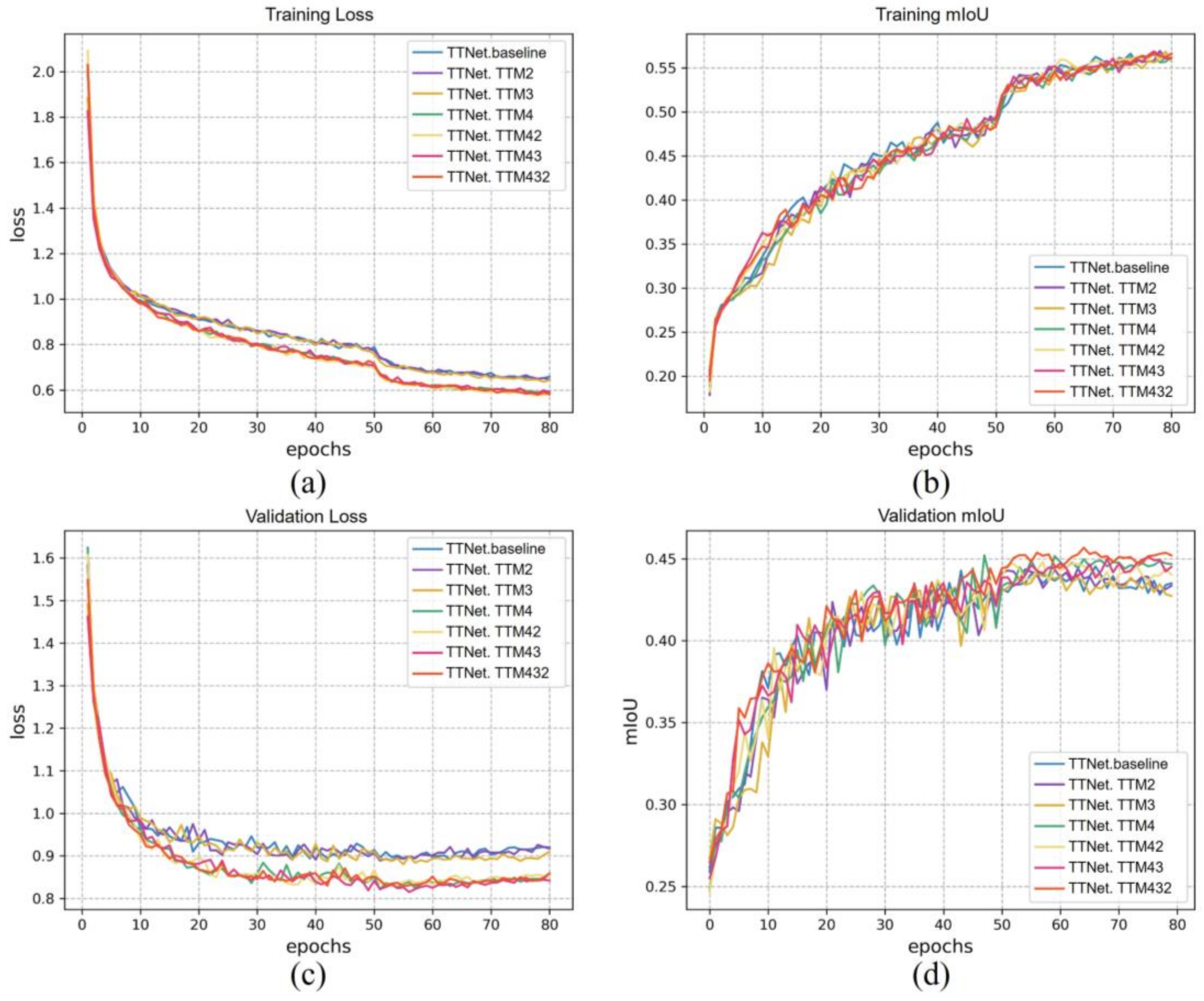
In Figure 11, we have illustrated the semantic metric curves derived from the seven ablation experiments during the training and validation phases. Observing Figure 11a,c, it becomes apparent that when compared to TTNet.baseline, both the training and validation semantic losses of TTNet.TTM432, TTNet.TTM43, and TTNet.TTM42 exhibit steeper descents with lower values as these models converge. In line with this trend, the validation semantic mIoU of these three models is higher. Furthermore, TTNet.TTM2 and TTNet.TTM3 exhibit performance comparable to TTNet in terms of both mIoU and loss. The insights drawn from the semantic metric curves align with our experimental findings and the preceding analysis.

4.5.2. Evaluation of TTM Design

We conducted a more in-depth exploration of the TTM architecture design, as presented in

Table 6. Ablation experiment results on TTM design based on SECOND 968 test set. The “√” symbol indicates whether actual labels of changed areas were used to derive the semantic change results. The best values are marked in bold.

Method	Label	mIoU(%)	$∆$
TTNet.baseline		44.43	-
+CAT		44.49	0.06
+TTM		45.91	1.48
TTNet.baseline	√	62.28	-
+CAT	√	65.04	2.76
+TTM	√	65.36	3.08

. An intuitive approach to capturing the change relationship is through Concatenation (CAT), wherein feature maps from the two bi-temporal images are concatenated and processed through a 1 × 1 convolutional layer to reduce channel dimensions. The results depicted in the last three rows of Table 6 reveal that both the CAT and TTM designs significantly enhance the baseline’s performance when semantic change maps are derived from the actual labels of binary change maps. Notably, the integration of TTM boosts the baseline’s mIoU by 3.08%. This emphasizes the significance of capturing change relationships through the fusion of bi-temporal image features, ultimately improving the accuracy of land cover classification for individual temporal images.

When actual labels of binary change areas are not employed to generate semantic change detection results, the performance of the CAT structure closely aligns with the baseline. This might be due to the fact that the CAT structure concatenates dual-temporal features, which does capture change relationships between the two temporal phases. However, this approach might inadvertently reduce the distinctiveness between these features, thereby diminishing the binary change detection branch’s performance. On the other hand, the TTM structure captures change relationships by calculating the similarity between dual-temporal features. This approach enables raw features to complement change information while better retaining feature differences.

4.5.3. TTM Weight Sharing Analysis

Given that TTM must be inserted into two separate semantic segmentation branches to capture the enhancements associated with the bidirectional change relationship, we examine whether TTM should share its weight across both branches. We present the findings of our ablation experiments in

Table 7. Ablation experiment results on TTM weight sharing on the SECOND 968 test set. The “√” symbol in “Share” column indicates the utilization of identical weights for TTM in both semantic segmentation branches. The “√” symbol in “Label” column indicates whether actual labels of changed areas were used to derive the semantic change results. The best values are marked in bold.

Method	Share	Label	mIoU(%)	$∆$
TTNet.baseline			44.43	-
+TTM			44.70	0.37%
+TTM	√		45.91	1.48%
TTNet.baseline		√	62.28	-
+TTM		√	64.57	2.29%
+TTM	√	√	65.36	3.08%

. The results from Table 7 clearly demonstrate that TTM with shared weights outperforms its counterpart with non-shared weights in both overall semantic change detection performance and semantic segmentation performance. This suggests that TTM with shared weights across both semantic segmentation branches can acquire more robust and representative features, benefiting from the simultaneous consideration of the bidirectional change relationship.

5. Conclusions

This paper argues that the change relationship among distinct temporal remote sensing images holds a pivotal role in the context of semantic change detection. It can significantly improve the distinguishability of raw features and effectively mitigate the mis-detection and un-detection challenges encountered in conventional post-classification techniques. To address this, we introduced the Temporal-Transformation Module designed to capture the change relationship through similarity calculations between features extracted from bi-temporal images. Concurrently, we devised a novel end-to-end fully convolutional network named TTNet, integrating multiple TTMs with shared weights into two semantic segmentation branches to effectively model bi-directional change relationships. The experimentation conducted on the SECOND dataset has demonstrated the superior performance of TTNet over several benchmark methods in semantic change detection tasks, underscoring the efficacy of incorporating change relationships in SCD methodologies.

The proposed approach, with its focus on capturing bi-directional change relationships in remote sensing imagery, holds promising implications for various applications. By refining the TTM design, optimizing TTNet architecture, and exploring multi-source data integration, this approach could be tailored to diverse environmental monitoring scenarios, from tracking urban development to detecting changes in agricultural landscapes. The implications also extend beyond the realm of remote sensing. For instance, the ability to capture intricate change relationships between images has potential applications in fields such as medical imaging, security surveillance, and autonomous systems.

However, it is important to acknowledge that while our approach shows promise, it is not a one-size-fits-all solution. The effectiveness of TTNet may vary across different datasets, geographical regions, spectrum bands, or types of land cover changes. Different datasets may yield varying results, as TTNet’s effectiveness is tied to the types of land cover changes within the dataset. For instance, it may excel in detecting certain change patterns, such as urban development, but its performance might be less optimal when confronted with other types of changes. A broader exploration of diverse change patterns is needed to comprehensively evaluate its capabilities. Additionally, the study’s robustness to noisy input data should be further examined to assess its applicability in less controlled environments. TTNet’s performance may be influenced by factors such as image quality, cloud cover, and seasonal variations, all of which can impact the effectiveness of SCD algorithms.

Our work opens several promising avenues for future investigations. First, refining the TTM design and further optimizing TTNet architecture can potentially enhance its performance in various remote sensing applications. Second, incorporating advanced machine learning techniques, such as deep reinforcement learning or domain adaptation, could lead to even more robust SCD models. Third, exploring the integration of multi-source data, including SAR and optical imagery, could expand the applicability of our approach to diverse environmental monitoring scenarios.

References

1. Singh, A. Review Article Digital Change Detection Techniques Using Remotely-Sensed Data. Int. J. Remote Sens. 1989, 10, 989–1003. [Google Scholar] [CrossRef]
2. Rahman, M.S.; Di, L. The State of the Art of Spaceborne Remote Sensing in Flood Management. Nat. Hazards 2017, 85, 1223–1248. [Google Scholar] [CrossRef]
3. Si Salah, H.; Ait-Aoudia, S.; Rezgui, A.; Goldin, S.E. Change Detection in Urban Areas from Remote Sensing Data: A Multidimensional Classification Scheme. Int. J. Remote Sens. 2019, 40, 6635–6679. [Google Scholar] [CrossRef]
4. Singh, G.; Singh, S.; Sethi, G.K.; Sood, V. Detection and Mapping of Agriculture Seasonal Variations with Deep Learning–Based Change Detection Using Sentinel-2 Data. Arab. J. Geosci. 2022, 15, 825. [Google Scholar] [CrossRef]
5. Diakogiannis, F.I.; Waldner, F.; Caccetta, P.; Wu, C. ResUNet-a: A Deep Learning Framework for Semantic Segmentation of Remotely Sensed Data. ISPRS J. Photogramm. Remote Sens. 2020, 162, 94–114. [Google Scholar] [CrossRef]
6. Tan, Z.; Gao, M.; Li, X.; Jiang, L. A Flexible Reference-Insensitive Spatiotemporal Fusion Model for Remote Sensing Images Using Conditional Generative Adversarial Network. IEEE Trans. Geosci. Remote Sens. 2022, 60, 5601413. [Google Scholar] [CrossRef]
7. Cheng, G.; Zhou, P.; Han, J. Learning Rotation-Invariant Convolutional Neural Networks for Object Detection in VHR Optical Remote Sensing Images. IEEE Trans. Geosci. Remote Sens. 2016, 54, 7405–7415. [Google Scholar] [CrossRef]
8. Tan, Z.; Gao, M.; Yuan, J.; Jiang, L.; Duan, H. A Robust Model for MODIS and Landsat Image Fusion Considering Input Noise. IEEE Trans. Geosci. Remote Sens. 2022, 60, 5407217. [Google Scholar] [CrossRef]
9. Cao, Z.; Jiang, L.; Yue, P.; Gong, J.; Hu, X.; Liu, S.; Tan, H.; Liu, C.; Shangguan, B.; Yu, D. A Large Scale Training Sample Database System for Intelligent Interpretation of Remote Sensing Imagery. Geo-Spat. Inf. Sci. 2023. [Google Scholar] [CrossRef]
10. Ji, S.; Wei, S.; Lu, M. Fully Convolutional Networks for Multisource Building Extraction From an Open Aerial and Satellite Imagery Data Set. IEEE Trans. Geosci. Remote Sens. 2019, 57, 574–586. [Google Scholar] [CrossRef]
11. Zhang, C.; Yue, P.; Tapete, D.; Jiang, L.; Shangguan, B.; Huang, L.; Liu, G. A Deeply Supervised Image Fusion Network for Change Detection in High Resolution Bi-Temporal Remote Sensing Images. ISPRS J. Photogramm. Remote Sens. 2020, 166, 183–200. [Google Scholar] [CrossRef]
12. Tian, S.; Zhong, Y.; Zheng, Z.; Ma, A.; Tan, X.; Zhang, L. Large-Scale Deep Learning Based Binary and Semantic Change Detection in Ultra High Resolution Remote Sensing Imagery: From Benchmark Datasets to Urban Application. ISPRS J. Photogramm. Remote Sens. 2022, 193, 164–186. [Google Scholar] [CrossRef]
13. Zhu, Q.; Guo, X.; Deng, W.; Shi, S.; Guan, Q.; Zhong, Y.; Zhang, L.; Li, D. Land-Use/Land-Cover Change Detection Based on a Siamese Global Learning Framework for High Spatial Resolution Remote Sensing Imagery. ISPRS J. Photogramm. Remote Sens. 2022, 184, 63–78. [Google Scholar] [CrossRef]
14. Cui, F.; Jiang, J. MTSCD-Net: A Network Based on Multi-Task Learning for Semantic Change Detection of Bitemporal Remote Sensing Images. Int. J. Appl. Earth Obs. Geoinf. 2023, 118, 103294. [Google Scholar] [CrossRef]
15. Niu, Y.; Guo, H.; Lu, J.; Ding, L.; Yu, D. SMNet: Symmetric Multi-Task Network for Semantic Change Detection in Remote Sensing Images Based on CNN and Transformer. Remote Sens. 2023, 15, 949. [Google Scholar] [CrossRef]
16. Varghese, A.; Gubbi, J.; Ramaswamy, A.; Balamuralidhar, P. ChangeNet: A Deep Learning Architecture for Visual Change Detection. In Proceedings of the European Conference on Computer Vision (ECCV) Workshops, Munich, Germany, 8–14 September 2018; pp. 1–16. [Google Scholar]
17. Jiang, F.; Gong, M.; Zhan, T.; Fan, X. A Semisupervised GAN-Based Multiple Change Detection Framework in Multi-Spectral Images. IEEE Geosci. Remote Sens. Lett. 2020, 17, 1223–1227. [Google Scholar] [CrossRef]
18. Sun, S.; Mu, L.; Wang, L.; Liu, P. L-UNet: An LSTM Network for Remote Sensing Image Change Detection. IEEE Geosci. Remote Sens. Lett. 2022, 19, 8004505. [Google Scholar] [CrossRef]
19. Prabhakar, K.R.; Ramaswamy, A.; Bhambri, S.; Gubbi, J.; Babu, R.V.; Purushothaman, B. CDNet++: Improved Change Detection with Deep Neural Network Feature Correlation. In Proceedings of the 2020 International Joint Conference on Neural Networks (IJCNN), Glasgow, UK, 19–24 July 2020; pp. 1–8. [Google Scholar]
20. Mou, L.; Bruzzone, L.; Zhu, X.X. Learning Spectral-Spatial-Temporal Features via a Recurrent Convolutional Neural Network for Change Detection in Multispectral Imagery. IEEE Trans. Geosci. Remote Sens. 2019, 57, 924–935. [Google Scholar] [CrossRef]
21. Dong, R.; Pan, X.; Li, F. DenseU-Net-Based Semantic Segmentation of Small Objects in Urban Remote Sensing Images. IEEE Access 2019, 7, 65347–65356. [Google Scholar] [CrossRef]
22. Yang, K.; Xia, G.-S.; Liu, Z.; Du, B.; Yang, W.; Pelillo, M.; Zhang, L. Asymmetric Siamese Networks for Semantic Change Detection in Aerial Images. IEEE Trans. Geosci. Remote Sens. 2022, 60, 1–18. [Google Scholar] [CrossRef]
23. Cao, C.; Dragićević, S.; Li, S. Land-Use Change Detection with Convolutional Neural Network Methods. Environments 2019, 6, 25. [Google Scholar] [CrossRef]
24. Caye Daudt, R.; Le Saux, B.; Boulch, A.; Gousseau, Y. Multitask Learning for Large-Scale Semantic Change Detection. Comput. Vis. Image Underst. 2019, 187, 102783. [Google Scholar] [CrossRef]
25. Tian, S.; Ma, A.; Zheng, Z.; Zhong, Y. Hi-UCD: A Large-Scale Dataset for Urban Semantic Change Detection in Remote Sensing Imagery. arXiv 2020, arXiv:2011.03247. [Google Scholar] [CrossRef]
26. Interdonato, R.; Ienco, D.; Gaetano, R.; Ose, K. DuPLO: A DUal View Point Deep Learning Architecture for Time Series classification. ISPRS J. Photogramm. Remote Sens. 2019, 149, 91–104. [Google Scholar] [CrossRef]
27. Nilsson, D.; Sminchisescu, C. Semantic Video Segmentation by Gated Recurrent Flow Propagation. In Proceedings of the IEEE Conference on Computer Vision and Pattern Recognition, Salt Lake City, UT, USA, 18–22 June 2018; pp. 6819–6828. [Google Scholar]
28. Gadde, R.; Jampani, V.; Gehler, P.V. Semantic Video CNNs Through Representation Warping. In Proceedings of the IEEE International Conference on Computer Vision, Venice, Italy, 22–29 October 2017; pp. 4453–4462. [Google Scholar]
29. Ienco, D.; Interdonato, R.; Gaetano, R.; Ho Tong Minh, D. Combining Sentinel-1 and Sentinel-2 Satellite Image Time Series for Land Cover Mapping via a Multi-Source Deep Learning Architecture. ISPRS J. Photogramm. Remote Sens. 2019, 158, 11–22. [Google Scholar] [CrossRef]
30. Zhang, H.; Zhang, H.; Wang, C.; Xie, J. Co-Occurrent Features in Semantic Segmentation. In Proceedings of the 2019 IEEE/CVF Conference on Computer Vision and Pattern Recognition (CVPR), Long Beach, CA, USA, 15–20 June 2019; pp. 548–557. [Google Scholar]
31. Wang, X.; Girshick, R.; Gupta, A.; He, K. Non-Local Neural Networks. In Proceedings of the IEEE Conference on Computer Vision and Pattern Recognition, Salt Lake City, UT, USA, 18–22 June 2018; pp. 7794–7803. [Google Scholar]
32. Fu, J.; Liu, J.; Tian, H.; Li, Y.; Bao, Y.; Fang, Z.; Lu, H. Dual Attention Network for Scene Segmentation. In Proceedings of the IEEE/CVF Conference on Computer Vision and Pattern Recognition, Long Beach, CA, USA, 15–20 June 2019; pp. 3146–3154. [Google Scholar]
33. Nemmour, H.; Chibani, Y. Support Vector Machines for Automatic Multi-Class Change Detection in Algerian Capital Using Landsat TM Imagery. J. Indian Soc. Remote Sens. 2010, 38, 585–591. [Google Scholar] [CrossRef]
34. Volpi, M.; Tuia, D.; Bovolo, F.; Kanevski, M.; Bruzzone, L. Supervised Change Detection in VHR Images Using Contextual Information and Support Vector Machines. Int. J. Appl. Earth Obs. Geoinf. 2013, 20, 77–85. [Google Scholar] [CrossRef]
35. Blakeslee, B.; Savakis, A. LambdaNet: A Fully Convolutional Architecture for Directional Change Detection. In Proceedings of the IS&T International Symposium on Electronic Imaging: Imaging and Multimedia Analytics in a Web and Mobile World, Burlingame, CA, USA, 26 January 2020; Volume 32, pp. 1–7. [Google Scholar]
36. Saha, S.; Bovolo, F.; Bruzzone, L. Unsupervised Deep Change Vector Analysis for Multiple-Change Detection in VHR Images. IEEE Trans. Geosci. Remote Sens. 2019, 57, 3677–3693. [Google Scholar] [CrossRef]
37. Zhang, P.; Gong, M.; Zhang, H.; Liu, J.; Ban, Y. Unsupervised Difference Representation Learning for Detecting Multiple Types of Changes in Multitemporal Remote Sensing Images. IEEE Trans. Geosci. Remote Sens. 2019, 57, 2277–2289. [Google Scholar] [CrossRef]
38. Iino, S.; Ito, R.; Doi, K.; Imaizumi, T.; Hikosaka, S. CNN-Based Generation of High-Accuracy Urban Distribution Maps Utilising SAR Satellite Imagery for Short-Term Change Monitoring. Int. J. Image Data Fusion 2018, 9, 302–318. [Google Scholar] [CrossRef]
39. Cheng, W.; Zhang, Y.; Lei, X.; Yang, W.; Xia, G. Semantic Change Pattern Analysis. arXiv 2020, arXiv:2003.03492. [Google Scholar] [CrossRef]
40. He, K.; Zhang, X.; Ren, S.; Sun, J. Deep Residual Learning for Image Recognition. In Proceedings of the IEEE Conference on Computer Vision and Pattern Recognition, Las Vegas, NV, USA, 27–30 June 2016; pp. 770–778. [Google Scholar]
41. Chen, L.-C.; Zhu, Y.; Papandreou, G.; Schroff, F.; Adam, H. Encoder-Decoder with Atrous Separable Convolution for Semantic Image Segmentation. In Proceedings of the European Conference on Computer Vision (ECCV), Munich, Germany, 8–14 September 2018; pp. 801–818. [Google Scholar]
42. Zhao, H.; Shi, J.; Qi, X.; Wang, X.; Jia, J. Pyramid Scene Parsing Network. In Proceedings of the IEEE Conference on Computer Vision and Pattern Recognition (CVPR), Honolulu, HI, USA, 21–26 July 2017; pp. 6230–6239. [Google Scholar]
Figure 1. The proportions of different change types within the SECOND dataset: (a) The proportions from T1 (image taken at the 1st timestamp) to T2 (image taken at the 2nd timestamp); and (b) the proportions from T2 to T1. This graph illustrates the proportions of different land cover classes appearing in another temporal image when the corresponding land cover class disappears in a specific temporal image. The X-axis represents the land cover class, while the Y-axis indicates the proportion.
Remotesensing 15 04555 g001
Figure 2. An overview of the proposed Temporal-Transform Network.
Remotesensing 15 04555 g002
Figure 3. The structure of Temporal-Transform Module (TTM).
Remotesensing 15 04555 g003
Figure 4. A selection of samples from the SECOND dataset.
Remotesensing 15 04555 g004
Figure 5. Visual comparison of undetected changes using the predicted binary change map on SECOND 968 test set. Enhanced regions highlighted with red and yellow dashed boxes. Yellow signifies regions where all methods exhibit correct detection, whereas red highlights regions where the benchmark methods yield inaccurate predictions.
Remotesensing 15 04555 g005
Figure 6. Visual Comparison of mis-detected changes based on the predicted binary change map on SECOND 968 test set. Improved areas marked with red and yellow dashed boxes. Yellow represents areas where all methods correctly detect changes, whereas red indicates areas where the benchmark methods’ predictions are incorrect.
Remotesensing 15 04555 g006
Figure 7. Visual comparison of undetected changes with labeled binary change map on SECOND 968 test set. Enhanced regions highlighted with red and yellow dashed boxes. Yellow signifies regions where all methods correctly detect changes, while red represents regions where the benchmark methods’ predictions are incorrect.
Remotesensing 15 04555 g007
Figure 8. Visual comparison of mis-detected changes with labeled binary change map on SECOND 968 test set. Improved areas marked with red and yellow dashed boxes. Yellow represents areas where all methods correctly detect changes, whereas red indicates areas where the benchmark methods’ predictions are incorrect.
Remotesensing 15 04555 g008
Figure 9. Visual comparison examples based on the labeled binary change map for the un-detection problem. Enhanced regions highlighted with red and yellow dashed boxes. Yellow represents areas where all network configurations yield comparable results, whereas red indicates areas where TTNet.TTM432 outperforms others.
Remotesensing 15 04555 g009
Figure 10. Visual comparison examples based on the labeled binary change map for the mis-detection problem. Improved areas marked with red and yellow dashed boxes. Yellow represents areas where all network configurations yield comparable results, whereas red indicates areas where TTNet.TTM432 outperforms others.
Remotesensing 15 04555 g010
Figure 11. Comparison of the training and validation semantic metric curves on the SECOND dataset: (a) training semantic loss; (b) training semantic mIoU; (c) validation semantic loss; and (d) validation semantic mIoU.
Remotesensing 15 04555 g011