


Incorporating Attention Mechanism, Dense Connection Blocks, and Multi-Scale Reconstruction Networks for Open-Set Hyperspectral Image Classification


Abstract
:
1. Introduction
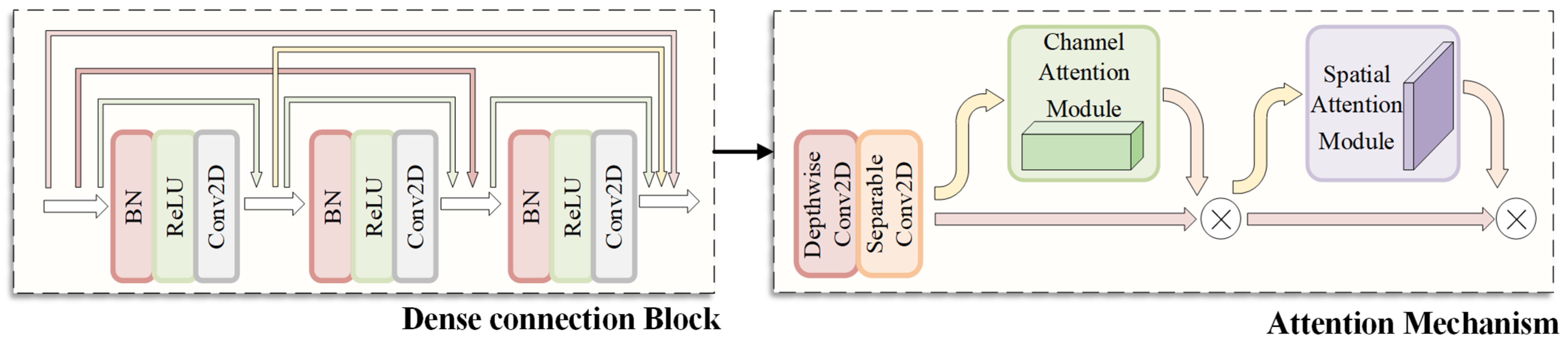
- We propose a novel feature extraction network model structure composed of dense connection blocks combined with an attention mechanism. It builds the connection relationship between different layers to make optimal use of features and mitigate the gradient disappearance problem. By using the channel attention module and the space attention module, you can solve the problem of what to focus on and where to focus on in the channel and spatial dimensions. Additionally, we enhance the attention mechanism model by bringing in a depthwise separable convolution, which reinforces the attention allocation in spatial and channel dimensions by splitting the correlation between spatial and channel dimensions. It promotes the feature formulation ability during forward propagation of the network and sufficiently extracts the feature information of small targets.
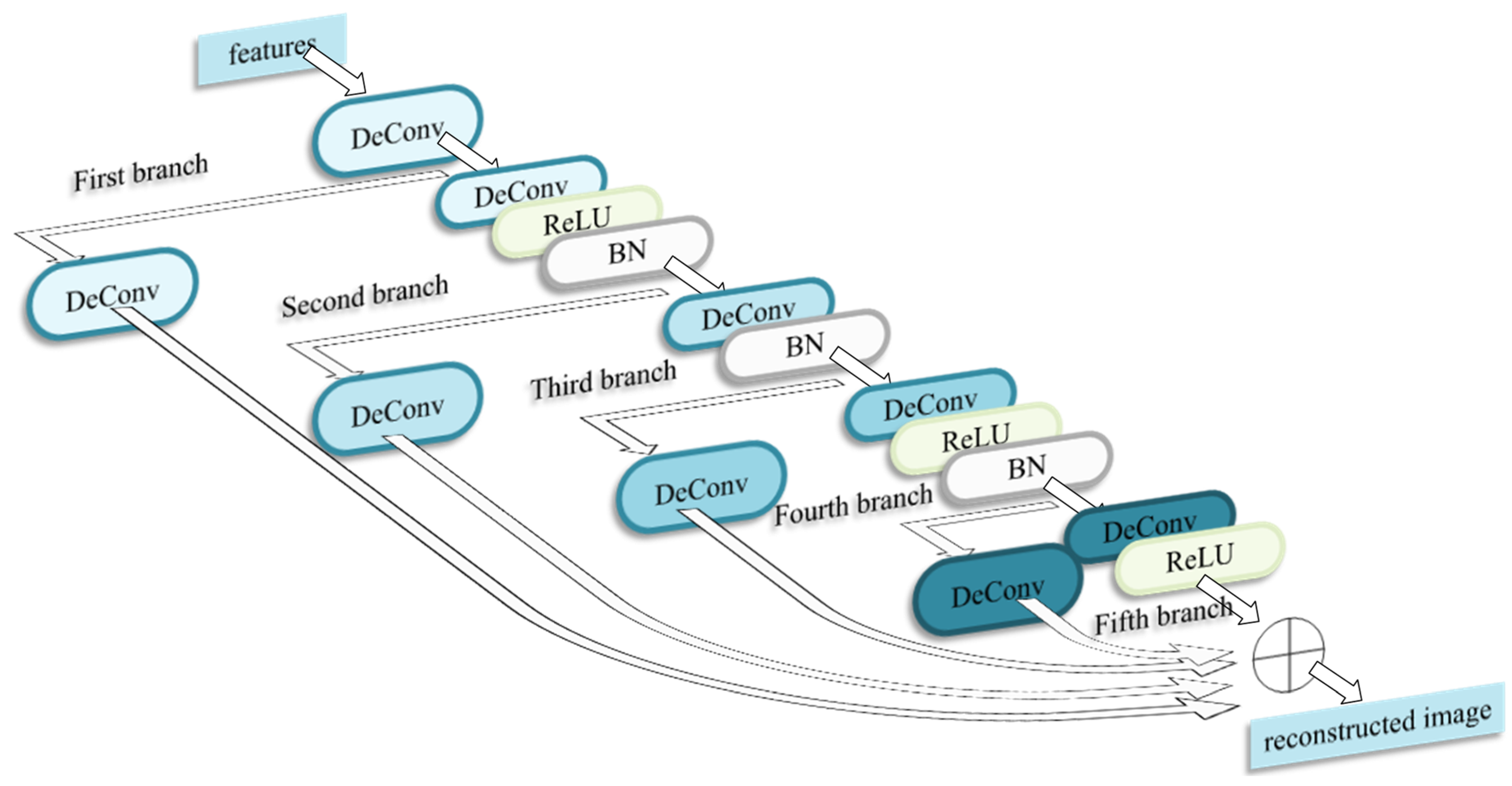
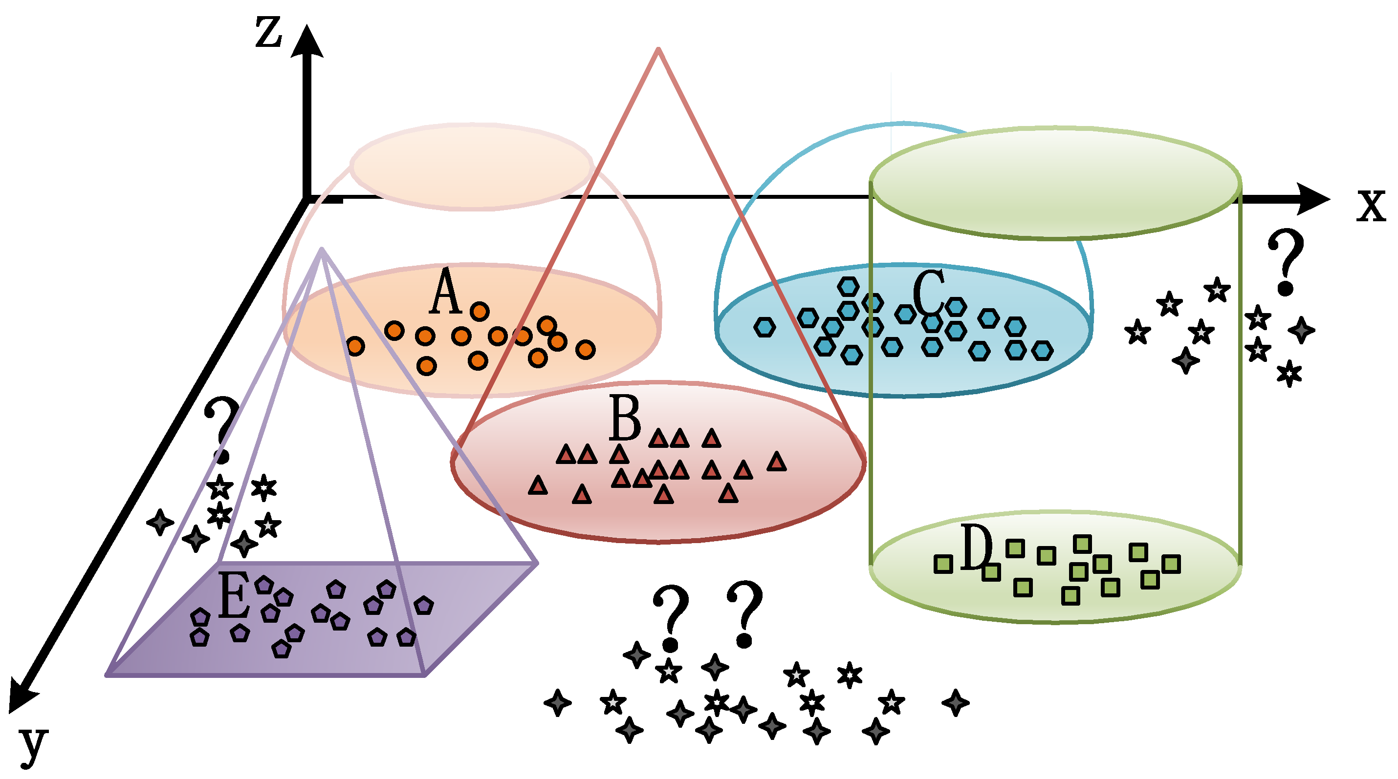
- We harness multi-task learning to perform classification and reconstruction simultaneously, thus permitting automatic identification of unknown classes. Deconvolutional filters with different sizes reconstruct different semantic information. Therefore, a multi-scale feature reconstruction architecture is introduced, which reconstructs the spatial context at multiple scales, thereby making full use of the rich spatial information and enhancing the robustness of the feature reconstruction in a complex background. Additionally, the multi-scale reconstruction network based on deconvolution helps to recover fine-grained details lost during feature extraction. The model further incorporates a multi-scale DeConv layer to fuse together and bolster the reconstructed network, rendering the reconstructed images intact and raising the classification accuracy.
- Experiments were evaluated on the Salinas, University of Pavia, and Indian Pines datasets. It demonstrates that the proposed method can obtain superior classification performance for the known class and unknown classes compared to other state-of-the-art classification methods.
- The rest of this article is organized as follows: Section 2 describes our proposed classification approach in detail. Section 3 reports the experimental results and evaluates the performance of the proposed method. It also analyzes the selection of experimental parameters in Section 4. Section 5 gives the conclusion.
2. Methodology
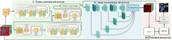
2.1. The Proposed IADMRN Framework for Open-Set HSI Classification
2.2. Feature Extraction Sub-Network
2.2.1. Dense Connection Block
2.2.2. Depthwise Separable Convolution Attention Mechanism
2.2.3. The Structure of Feature Extraction Sub-Network
2.3. Image Reconstruction Sub-Network
2.4. Classification Sub-Network
2.4.1. Reconstruction Loss Calculation
2.4.2. EVT Extreme Value Modeling
2.4.3. Threshold-Based Classification Decision
3. Results
3.1. Datasets Description
- (1)
- Salinas: The Salinas dataset is named after the Salinas Valley in California, USA, where the data were collected. The dataset provides high-resolution hyperspectral images captured by an airborne sensor, containing detailed spectral and spatial information about the agricultural region [35,36]. The Salinas dataset consists of 512 × 217 pixels, with a total of 224 spectral bands covering the wavelength range from 0.2 to 2.4 μm. In addition, some unannotated man-made materials have been annotated as unknown samples, and the reference map contains 17 classes in total. The number of classes is presented in Table 1.
- (2)
- University of Pavia: The University of Pavia dataset is an extensively accessible hyperspectral remote sensing dataset, commonly adopted in the field of hyperspectral image analysis and classification. It was gathered by the Reflection Optical System Imaging Spectrometer (ROSIS) sensor in an agricultural area of Pavia, Italy. The dataset delivers high spatial resolution and covers a vast spectral range, yielding valuable information for a variety of land cover and land use applications [37]. It incorporates 103 bands after filtering out the 12 bands affected by noise and water absorption, with a scene size of 610 × 340 and a GSD of 1.3 m. Additionally, some buildings left unannotated are marked as unknown. They share distinct spectral profiles with the known land cover, and the reference map contains 10 classes. The detailed number of pixels available in each class, the false-color composite image, and the ground truth map are presented in Table 2.
- (3)
- Indian Pines: The Indian Pines dataset provides both spatial and spectral information about the captured scene. It consists of a 145 × 145 pixel spatial resolution, meaning it contains 21,025 pixels in total. Each pixel in the dataset represents a hyperspectral signature containing spectral reflectance information across 145 different bands [38]. The Indian Pines dataset encompasses a diverse set of land cover classes, including crops, vegetation, bare soil, and man-made structures. It contains a total of 16 different land cover classes, making it suitable for various classification and analysis tasks. Since the number of instantiations was less than 10 for part classes, these tail classes were discarded in the experiments following the paper [35] and regarded as unknown classes, leading to 8 known classes. Details of the dataset can be found in Table 3.
3.2. Experimental Parameters Setting
- (1)
- Implementation Details: All experiments were performed on an Intel(R) Xeon(R) 4208 CPU @ 2.10 GHz processor and Nvidia GeForce RTX 2080Ti graphics card. The AdaDelta optimizer is used for backpropagation in the training phase. The learning rate was set at 1.0 for the first 170 epochs and then at 0.1 for another 30 epochs before the training stopped. We adopted the early stopping mechanism to accelerate the training. If the loss does not decrease for five epochs, the learning proceeds immediately to the next phase.
- (2)
- Evaluation Indexes: Three widely used objective indexes, that is, overall accuracy (OA), average accuracy (AA), and Kappa coefficient, are adopted to verify the classification effect of all methods. All objective results are listed by calculating the average of ten random training samples.
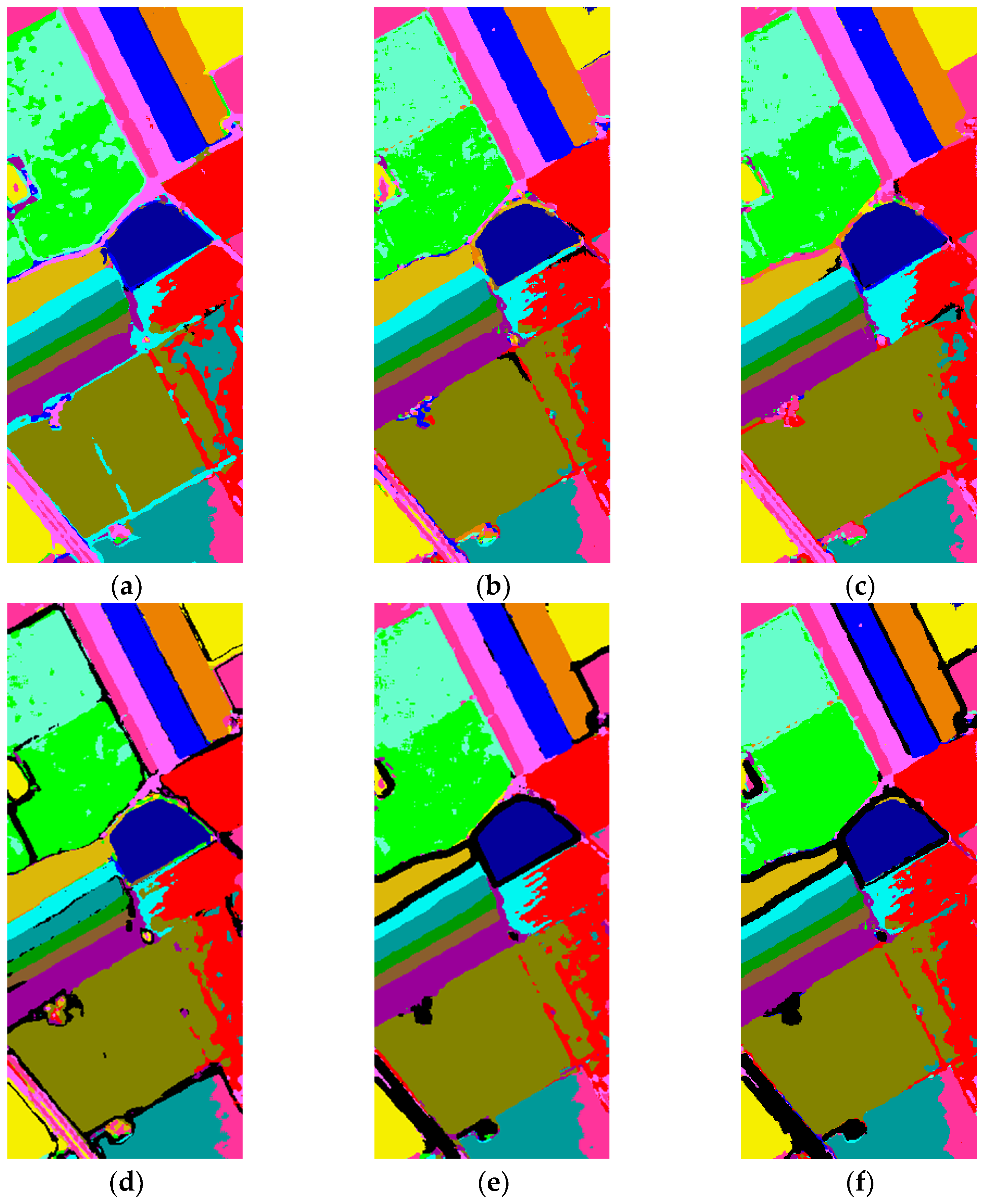
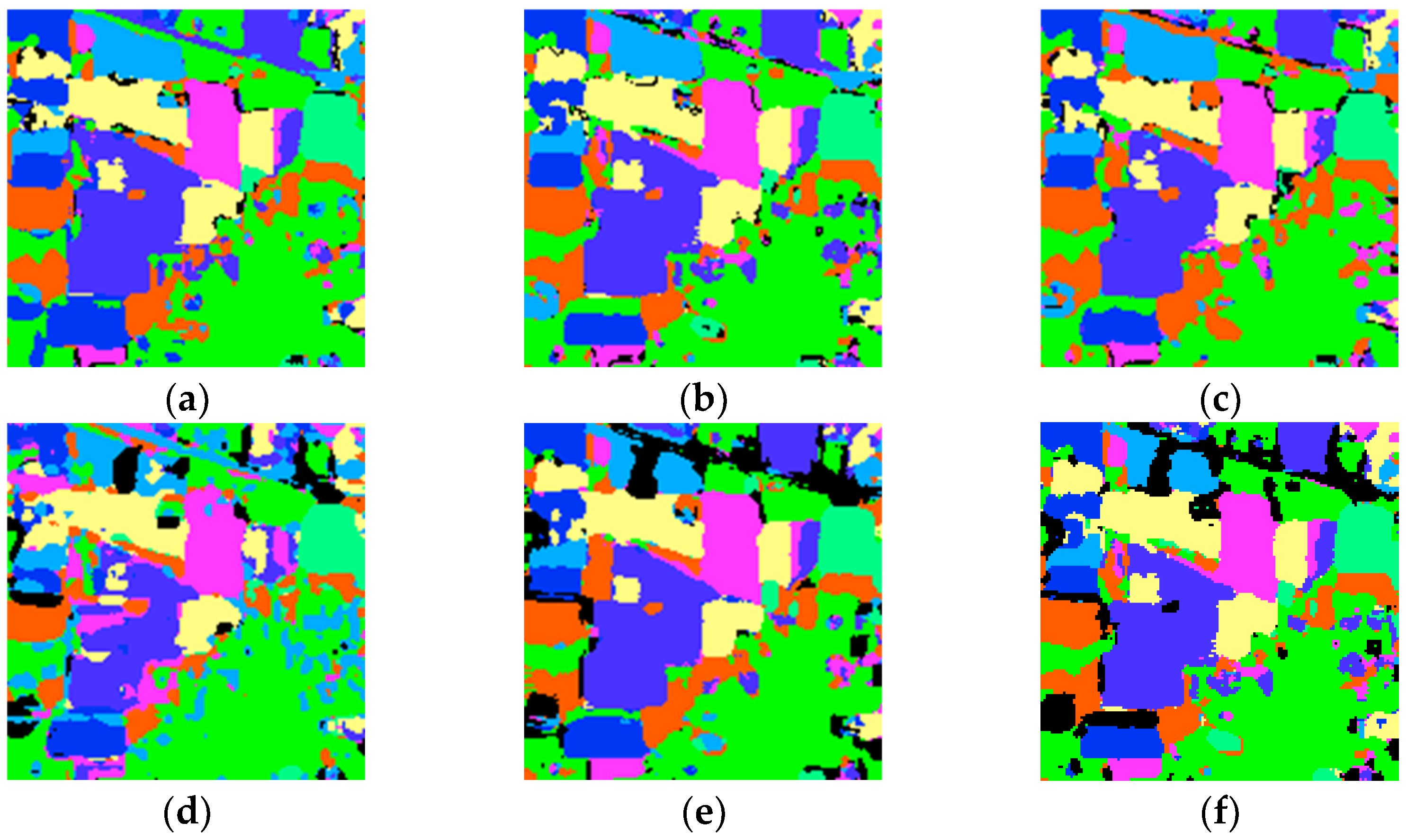
3.3. Comparison of the Proposed Methods with the State-of-the-Art Methods
4. Discussion
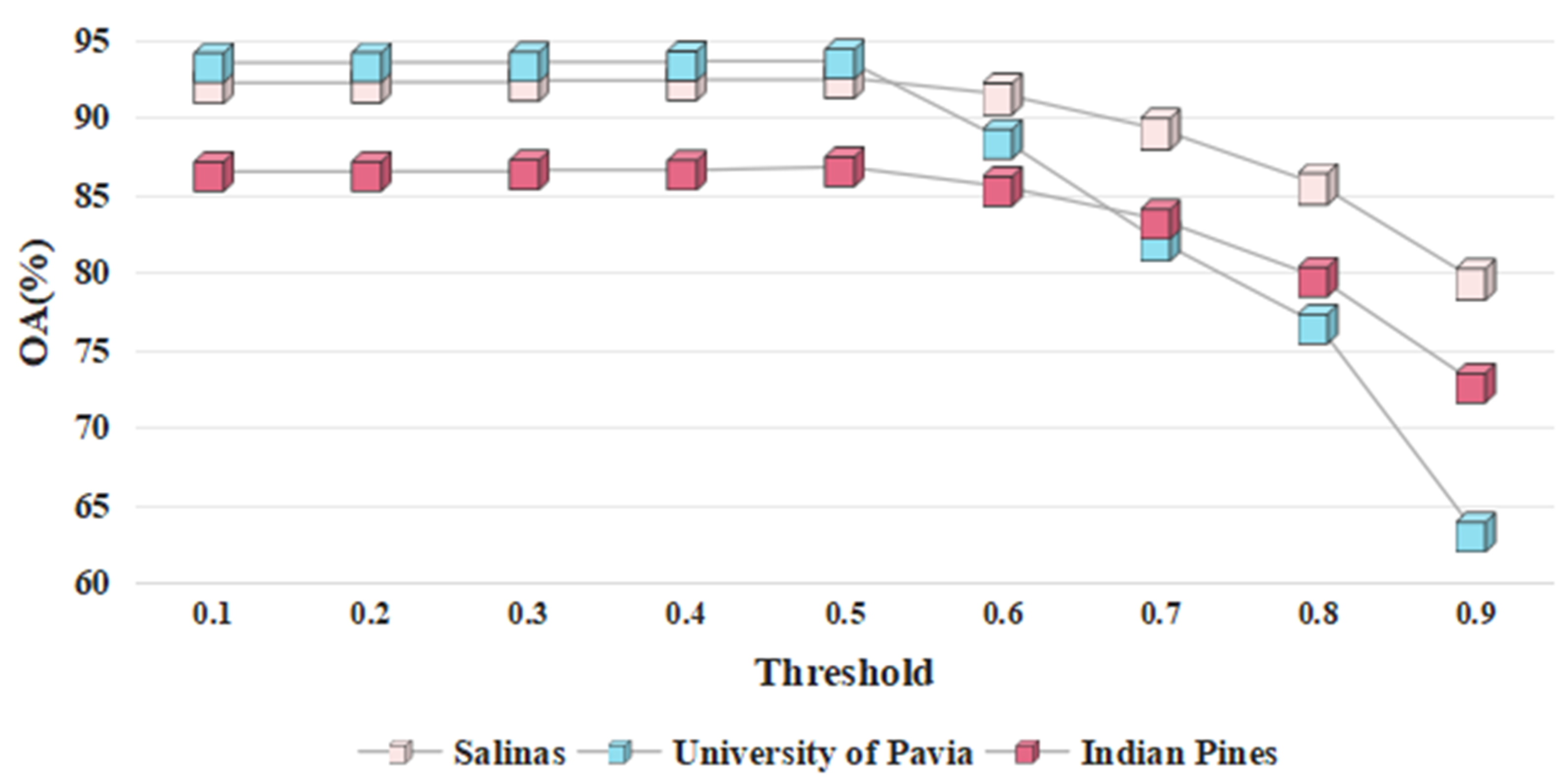
4.1. The Threshold of SoftMax
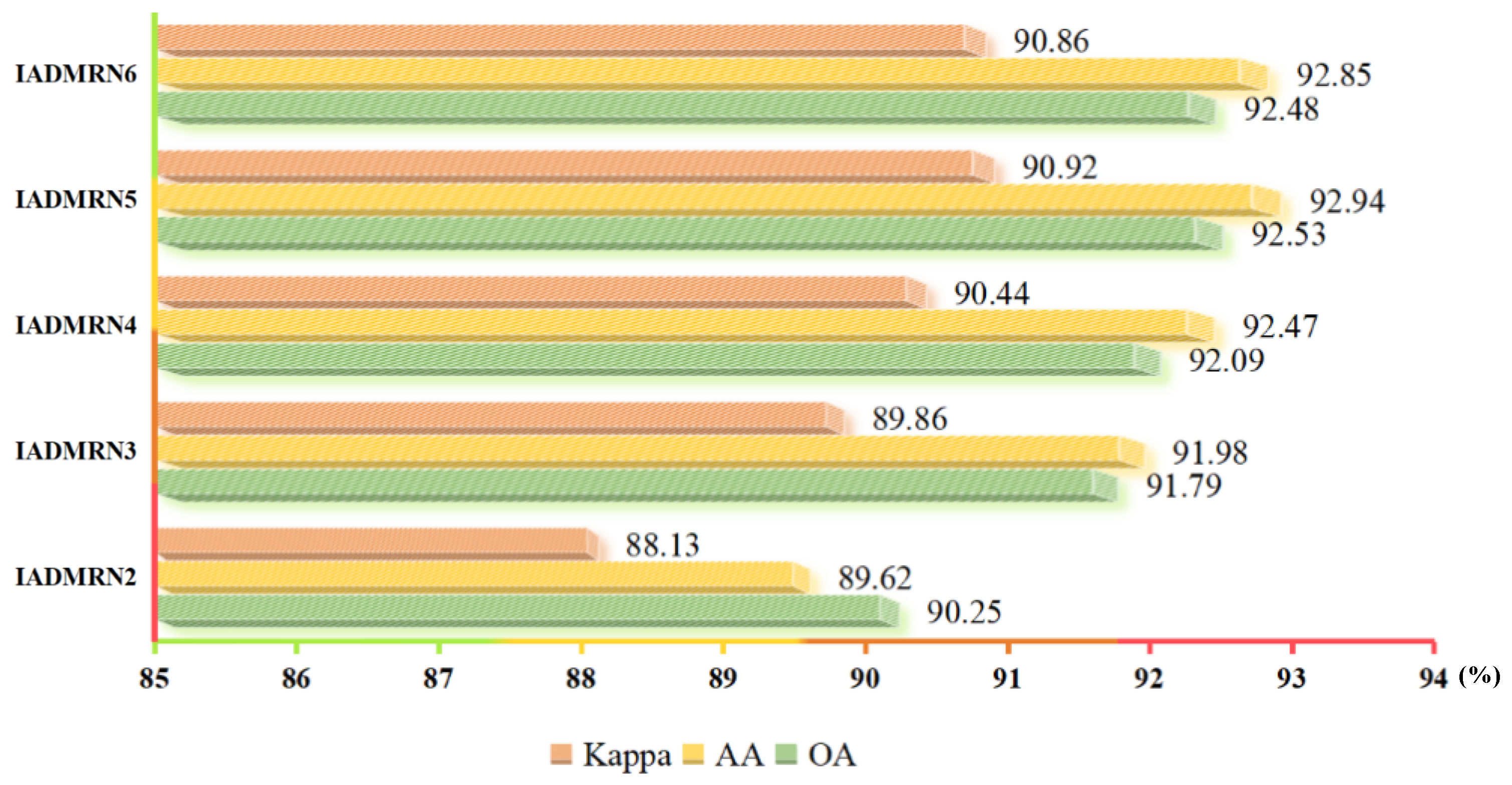
4.2. The Number of Branches in Feature Fusion Strategy
4.3. Ablation Study
5. Conclusions
Author Contributions
Funding
Data Availability Statement
Conflicts of Interest
References
- Cao, X.; Yao, J.; Xu, Z.; Meng, D. Hyperspectral image classification with convolutional neural network and active learning. IEEE Trans. Geosci. Remote Sens. 2020, 58, 4604–4616. [Google Scholar] [CrossRef]
- Wang, L.; Shi, Y.; Zhang, Z. Hyperspectral Image Classification Combining Improved Local Binary Mode and Superpixel-level Decision. J. Signal Process. 2023, 39, 61–72. [Google Scholar] [CrossRef]
- Fang, L.; Zhu, D.; Yue, J.; Zhang, B.; He, M. Geometric-Spectral Reconstruction Learning for Multi-Source Open-Set Classification with Hyperspectral and LiDAR Data. IEEE/CAA J. Autom. Sin. 2022, 9, 1892–1895. [Google Scholar] [CrossRef]
- Imani, M.; Ghassemian, H. Principal component discriminant analysis for feature extraction and classification of hyperspectral images. In Proceedings of the 2014 Iranian Conference on Intelligent Systems (ICIS), Bam, Iran, 4–6 February 2014; pp. 1–5. [Google Scholar] [CrossRef]
- Yuan, H.; Lu, Y.; Yang, L.; Luo, H.; Tang, Y.Y. Spectral-spatial linear discriminant analysis for hyperspectral image classification. In Proceedings of the 2013 IEEE International Conference on Cybernetics (CYBCO), Lausanne, Switzerland, 13–15 June 2013; pp. 144–149. [Google Scholar] [CrossRef]
- Chen, Y.; Lin, Z.; Zhao, X.; Wang, G.; Gu, Y. Deep learning-based classification of hyperspectral data. IEEE J. Sel. Top. Appl. Earth Observ. Remote Sens. 2014, 7, 2094–2107. [Google Scholar] [CrossRef]
- Chen, Y.; Jiang, H.; Li, C.; Jia, X.; Ghamisi, P. Deep feature extraction and classification of hyperspectral images based on convolutional neural networks. IEEE Trans. Geosci. Remote Sens. 2016, 54, 6232–6251. [Google Scholar] [CrossRef]
- Zhong, Z.; Li, J.; Luo, Z.; Chapman, M. Spectral–spatial residual network for hyperspectral image classification: A 3-D deep learning framework. IEEE Trans. Geosci. Remote Sens. 2017, 56, 847–858. [Google Scholar] [CrossRef]
- Liu, Y.; Tang, Y.; Zhang, L.; Liu, L.; Song, M.; Gong, K.; Peng, Y.; Hou, J.; Jiang, T. Hyperspectral open set classification with unknown classes rejection towards deep networks. Int. J. Remote Sens. 2020, 41, 6355–6383. [Google Scholar] [CrossRef]
- Duan, Z.; Chen, H.; Li, X.; Zhou, J.; Wang, Y. A Semi-Supervised Learning Method for Hyperspectral-Image Open Set Classification. Photogramm. Eng. Remote Sens. 2022, 88, 653–664. [Google Scholar] [CrossRef]
- Pal, D.; Bundele, V.; Sharma, R.; Banerjee, B.; Jeppu, Y. Few-shotopen-set recognition of hyperspectral images with outlier calibration network. In Proceedings of the IEEE/CVF Winter Conference on Applications of Computer Vision (WACV), Waikoloa, HI, USA, 3–8 January 2022; pp. 3801–3810. [Google Scholar]
- Yue, J.; Fang, L.; He, M. Spectral-spatial latent reconstruction for open-set hyperspectral image classification. IEEE Trans. Image Process. 2022, 31, 5227–5241. [Google Scholar] [CrossRef]
- Xie, Z.; Duan, P.; Liu, W.; Kang, X.; Wei, X.; Li, S. Feature Consistency-Based Prototype Network for Open-Set Hyperspectral Image Classification. IEEE Trans. Neural Netw. Learn. Syst. 2023, 1–11. [Google Scholar] [CrossRef]
- Liu, Y.; Hou, J.; Peng, Y.; Jiang, T. Distance-based hyperspectral open-set classification of deep neural networks. Remote Sens. Lett. 2021, 12, 636–644. [Google Scholar] [CrossRef]
- Tang, X.; Peng, Y.; Li, C.; Zhou, T. Open set domain adaptation based on multi-classifier adversarial network for hyperspectral image classification. J. Appl. Remote Sens. 2021, 15, 044514. [Google Scholar] [CrossRef]
- Wen, C.; Hong, M.; Yang, X.; Jia, J. Pulmonary Nodule Detection Based on Convolutional Block Attention Module. In Proceedings of the 2019 Chinese Control Conference (CCC), Guangzhou, China, 27–30 July 2019; pp. 8583–8587. [Google Scholar] [CrossRef]
- Srivastava, H.; Sarawadekar, K. A Depthwise Separable Convolution Architecture for CNN Accelerator. In Proceedings of the 2020 IEEE Applied Signal Processing Conference (ASPCON), Kolkata, India, 7–9 October 2020; pp. 1–5. [Google Scholar]
- Liu, S.; Shi, Q.; Zhang, L. Few-shot hyperspectral image classification with unknown classes using multitask deep learning. IEEE Trans. Geosci. Remote Sens. 2020, 59, 5085–5102. [Google Scholar] [CrossRef]
- Liu, Y.; Hou, J.; Peng, Y.; Xu, Y.; Jiang, T. Hyperspectral Open Set Classification towards Deep Networks Based on Boxplot. IOP Conf. Ser. Earth Environ. Sci. 2021, 693, 012085. [Google Scholar] [CrossRef]
- Li, S.; Song, W.; Fang, L.; Chen, Y.; Ghamisi, P.; Benediktsson, J.A. Deep learning for hyperspectral image classification: An overview. IEEE Trans. Geosci. Remote Sens. 2019, 57, 6690–6709. [Google Scholar] [CrossRef]
- Camps-Valls, G.; Bruzzone, L. Kernel-based methods for hyperspectral image classification. IEEE Trans. Geosci. Remote Sens. 2005, 43, 1351–1362. [Google Scholar] [CrossRef]
- He, L.; Li, J.; Liu, C.; Li, S. Recent advances on spectral–spatial hyperspectral image classification: An overview and new guidelines. IEEE Trans. Geosci. Remote Sens. 2017, 56, 1579–1597. [Google Scholar] [CrossRef]
- Yang, X.; Ye, Y.; Li, X.; Lau, R.Y.; Zhang, X.; Huang, X. Hyperspectral image classification with deep learning models. IEEE Trans. Geosci. Remote Sens. 2018, 56, 5408–5423. [Google Scholar] [CrossRef]
- Chen, H.; Miao, F.; Chen, Y.; Xiong, Y.; Chen, T. A hyperspectral image classification method using multifeature vectors and optimized KELM. IEEE J. Sel. Top. Appl. Earth Obs. Remote Sens. 2021, 14, 2781–2795. [Google Scholar] [CrossRef]
- Hong, D.; Han, Z.; Yao, J.; Gao, L.; Zhang, B.; Plaza, A.; Chanussot, J. SpectralFormer: Rethinking hyperspectral image classification with transformers. IEEE Trans. Geosci. Remote Sens. 2021, 60, 5518615. [Google Scholar] [CrossRef]
- Hong, D.; Gao, L.; Yao, J.; Zhang, B.; Plaza, A.; Chanussot, J. Graph convolutional networks for hyperspectral image classification. IEEE Trans. Geosci. Remote Sens. 2020, 59, 5966–5978. [Google Scholar] [CrossRef]
- Mou, L.; Lu, X.; Li, X.; Zhu, X.X. Nonlocal graph convolutional networks for hyperspectral image classification. IEEE Trans. Geosci. Remote Sens. 2020, 58, 8246–8257. [Google Scholar] [CrossRef]
- Hang, R.; Li, Z.; Liu, Q.; Ghamisi, P.; Bhattacharyya, S.S. Hyperspectral image classification with attention-aided CNNs. IEEE Trans. Geosci. Remote Sens. 2020, 59, 2281–2293. [Google Scholar] [CrossRef]
- Wang, H.; Wang, A.C.; Cang, S. Hyperspectral remote sensing image reconstruction method based on compressive sensing. Chin. J. Liq. Cryst. Disp. 2017, 32, 219–226. [Google Scholar] [CrossRef]
- Guo, Y.L.; Li, Y.M.; Zhu, L.; Xu, D.Q.; Li, Y.; Tan, J.; Zhou, L.; Liu, G. Research of hyperspectral reconstruction based on HJ1A-CCD data. Huan Jing ke Xue = Huanjing Kexue 2013, 34, 69–76. [Google Scholar]
- He, X.; Chen, Y.; Lin, Z. Spatial-spectral transformer for hyperspectral image classification. Remote Sens. 2021, 13, 498. [Google Scholar] [CrossRef]
- Rudd, E.M.; Jain, L.P.; Scheirer, W.J.; Boult, T.E. The Extreme Value Machine. IEEE Trans. Pattern Anal. Mach. Intell. 2018, 40, 762–768. [Google Scholar] [CrossRef]
- Pal, D.; Bose, S.; Banerjee, B.; Jeppu, Y. Extreme Value Meta-Learning for Few-Shot Open-Set Recognition of Hyperspectral Images. IEEE Trans. Geosci. Remote Sens. 2023, 61, 5512516. [Google Scholar] [CrossRef]
- Sawant, S.S.; Manoharan, P. Unsupervised band selection based on weighted information entropy and 3D discrete cosine transform for hyperspectral image classification. Int. J. Remote Sens. 2020, 41, 3948–3969. [Google Scholar] [CrossRef]
- Lee, H.; Kwon, H. Going deeper with contextual CNN for hyperspectral image classification. IEEE Trans. Image Process. 2017, 26, 4843–4855. [Google Scholar] [CrossRef]
- Zhong, Z.; Li, J.; Ma, L.; Jiang, H.; Zhao, H. Deep residual networks for hyperspectral image classification. In Proceedings of the 2017 IEEE International Geoscience and Remote Sensing Symposium (IGARSS), Fort Worth, TX, USA, 23–28 July 2017; pp. 1824–1827. [Google Scholar]
- Bhosle, K.; Musande, V. Evaluation of deep learning CNN model for land use land cover classification and crop identification using hyperspectral remote sensing images. J. Indian Soc. Remote Sens. 2019, 47, 1949–1958. [Google Scholar] [CrossRef]
- Li, Q.; Wong FK, K.; Fung, T. Mapping multi-layered mangroves from multispectral, hyperspectral, and LiDAR data. Remote Sens. Environ. 2021, 258, 112403. [Google Scholar] [CrossRef]
- Morchhale, S.; Pauca, V.P.; Plemmons, R.J.; Torgersen, T.C. Classification of pixel-level fused hyperspectral and lidar data using deep convolutional neural networks. In Proceedings of the 2016 8th Workshop on Hyperspectral Image and Signal Processing: Evolution in Remote Sensing (WHISPERS), Los Angeles, CA, USA, 21–24 August 2016; pp. 1–5. [Google Scholar]
- Liu, X.; Meng, Y.; Fu, M. Classification Research Based on Residual Network for Hyperspectral Image. In Proceedings of the 2019 IEEE 4th International Conference on Signal and Image Processing (ICSIP), Wuxi, China, 19–21 July 2019; pp. 911–915. [Google Scholar]
- Li, Z.; Liu, M.; Chen, Y.; Xu, Y.; Li, W.; Du, Q. Deep Cross-Domain Few-Shot Learning for Hyperspectral Image Classification. IEEE Trans. Geosci. Remote Sens. 2021, 60, 5501618. [Google Scholar] [CrossRef]
- Krishnendu, C.S.; Sowmya, V.; Soman, K.P. Impact of Dimension Reduced Spectral Features on Open Set Domain Adaptation for Hyperspectral Image Classification. In Evolution in Computational Intelligence; Bhateja, V., Peng, S.L., Satapathy, S.C., Zhang, Y.D., Eds.; Advances in Intelligent Systems and Computing; Springer: Singapore, 2021; Volume 1176. [Google Scholar] [CrossRef]


| No | Name | Color | Number | Ground-Truth Map | False-Color Map |
|---|---|---|---|---|---|
| 1 | Weeds-2 | 3726 |  |  | |
| 2 | Stubble | 3979 | |||
| 3 | Lettuce-4wk | 1068 | |||
| 4 | Vinyard-U | 7268 | |||
| 5 | Lettuce-5wk | 1927 | |||
| 6 | Lettuce-6wk | 916 | |||
| 7 | Grapes | 11,271 | |||
| 8 | Vinyard-T | 1807 | |||
| 9 | Weeds-1 | 2009 | |||
| 10 | Celery | 3579 | |||
| 11 | Fallow | 1976 | |||
| 12 | Fallow-P | 1394 | |||
| 13 | Fallow-S | 2678 | |||
| 14 | Corn | 3278 | |||
| 15 | Lettuce-7wk | 1070 | |||
| 16 | Soil | 6203 | |||
| 17 | Unknown | 5613 | |||
| Total Numbers | 59,742 | ||||
| No | Name | Color | Number | Ground-Truth Map | False-Color Map |
|---|---|---|---|---|---|
| 1 | Asphalt | 6631 |  | 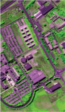 | |
| 2 | Meadows | 18,649 | |||
| 3 | Gravel | 2099 | |||
| 4 | Trees | 3064 | |||
| 5 | Metal S. | 1345 | |||
| 6 | Bare S. | 5029 | |||
| 7 | Bitumen | 1330 | |||
| 8 | Brick | 3682 | |||
| 9 | Shadow | 947 | |||
| 10 | Unknown | 5163 | |||
| Total Numbers | 47,939 | ||||
| No | Name | Color | Number | Ground-Truth Map | False-Color Map |
|---|---|---|---|---|---|
| 1 | Corn-notill | 1428 |  | 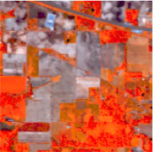 | |
| 2 | Corn-mintill | 830 | |||
| 3 | Grass-pasture | 483 | |||
| 4 | Haywindrowed | 478 | |||
| 5 | Soybean-notill | 972 | |||
| 6 | Soybean-mintill | 2454 | |||
| 7 | Soybean-clean | 593 | |||
| 8 | Woods | 1265 | |||
| 9 | Unknown | 2007 | |||
| Total Numbers | 10,510 | ||||
| Classes | CNN | ResNet | DCFSL | OS-GAN | MDL4OW | IADMRN |
|---|---|---|---|---|---|---|
| Weeds-1 | 82.16 | 81.22 | 85.47 | 87.76 | 90.41 | 91.75 |
| Weeds-2 | 86.02 | 87.38 | 90.51 | 91.65 | 93.27 | 94.52 |
| Fallow | 90.25 | 89.16 | 92.04 | 94.07 | 95.71 | 96.94 |
| Fallow-P | 87.43 | 86.31 | 89.68 | 93.88 | 96.52 | 97.50 |
| Fallow-S | 77.29 | 79.03 | 84.75 | 83.27 | 86.81 | 87.44 |
| Stubble | 85.97 | 86.27 | 88.01 | 90.43 | 92.35 | 93.12 |
| Celery | 89.42 | 88.69 | 92.26 | 91.72 | 93.54 | 94.87 |
| Grapes | 71.03 | 72.64 | 74.19 | 76.96 | 80.14 | 82.21 |
| Soil | 89.64 | 90.55 | 93.13 | 92.75 | 96.06 | 97.83 |
| Corn | 85.21 | 87.94 | 91.27 | 93.41 | 93.15 | 94.06 |
| Lettuce-4wk | 84.16 | 83.08 | 86.39 | 89.02 | 93.76 | 95.21 |
| Lettuce-5wk | 83.29 | 85.45 | 90.84 | 93.08 | 95.73 | 96.64 |
| Lcttuce-6wk | 87.39 | 88.06 | 92.67 | 95.13 | 97.07 | 98.45 |
| Lcttuce-7wk | 88.34 | 87.24 | 90.64 | 95.94 | 96.32 | 97.81 |
| Vinyard-U | 73.61 | 69.21 | 78.65 | 80.06 | 81.13 | 83.19 |
| Vinyard-T | 87.12 | 88.13 | 90.59 | 92.37 | 94.25 | 96.95 |
| Unknown | 1.51 | 3.02 | 4.87 | 32.45 | 61.84 | 80.76 |
| OA (%) | 78.14 | 79.54 | 82.34 | 84.06 | 88.18 | 92.53 |
| AA (%) | 82.16 | 83.06 | 85.12 | 87.64 | 91.87 | 92.94 |
| Kappa (%) | 71.43 | 72.18 | 77.91 | 81.29 | 86.32 | 90.92 |
| Classes | CNN | ResNet | DCFSL | OS-GAN | MDL4OW | IADMRN |
|---|---|---|---|---|---|---|
| Asphalt | 78.21 | 85.43 | 88.46 | 89.24 | 91.32 | 93.59 |
| Meadows | 82.72 | 87.05 | 92.12 | 93.17 | 92.05 | 93.48 |
| Gravel | 84.56 | 86.61 | 89.37 | 91.56 | 93.79 | 97.52 |
| Trees | 85.09 | 89.03 | 92.05 | 91.28 | 93.52 | 95.16 |
| Metal S. | 76.10 | 78.85 | 86.53 | 88.74 | 87.31 | 89.91 |
| Bare S. | 77.21 | 83.49 | 89.46 | 91.59 | 91.07 | 95.35 |
| Bitumen | 80.43 | 83.12 | 87.91 | 88.63 | 90.62 | 92.06 |
| Brick | 75.15 | 76.59 | 83.19 | 82.04 | 86.51 | 89.19 |
| Shadow | 80.64 | 78.17 | 82.59 | 85.17 | 83.84 | 87.57 |
| Unknown | 1.79 | 2.41 | 3.35 | 31.61 | 57.84 | 79.23 |
| OA (%) | 73.66 | 80.29 | 84.12 | 87.15 | 89.64 | 93.72 |
| AA (%) | 75.59 | 82.73 | 84.03 | 89.79 | 92.12 | 94.06 |
| Kappa (%) | 72.12 | 75.44 | 80.47 | 85.96 | 88.57 | 91.19 |
| Classes | CNN | ResNet | DCFSL | OS-GAN | MDL4OW | IADMRN |
|---|---|---|---|---|---|---|
| Asphalt | 70.03 | 77.27 | 86.21 | 89.42 | 91.13 | 92.18 |
| Meadows | 69.87 | 74.25 | 88.59 | 89.57 | 90.08 | 91.49 |
| Gravel | 72.15 | 76.13 | 81.34 | 84.95 | 83.71 | 85.47 |
| Trees | 82.06 | 87.05 | 91.71 | 93.01 | 96.57 | 97.08 |
| Metal S. | 84.64 | 86.90 | 88.65 | 87.29 | 90.54 | 91.35 |
| Bare S. | 77.98 | 85.36 | 89.20 | 91.82 | 93.39 | 94.86 |
| Bitumen | 80.75 | 85.22 | 84.46 | 85.53 | 87.76 | 90.71 |
| Brick | 78.02 | 81.14 | 83.25 | 84.76 | 87.21 | 89.02 |
| Unknown | 0.79 | 3.07 | 5.81 | 25.44 | 34.08 | 59.62 |
| OA (%) | 68.29 | 77.75 | 81.13 | 82.54 | 84.32 | 86.79 |
| AA (%) | 73.41 | 79.89 | 82.04 | 84.19 | 86.76 | 89.81 |
| Kappa (%) | 61.54 | 72.35 | 75.61 | 77.11 | 81.03 | 83.55 |
Disclaimer/Publisher’s Note: The statements, opinions and data contained in all publications are solely those of the individual author(s) and contributor(s) and not of MDPI and/or the editor(s). MDPI and/or the editor(s) disclaim responsibility for any injury to people or property resulting from any ideas, methods, instructions or products referred to in the content. |
© 2023 by the authors. Licensee MDPI, Basel, Switzerland. This article is an open access article distributed under the terms and conditions of the Creative Commons Attribution (CC BY) license (https://creativecommons.org/licenses/by/4.0/).
Share and Cite
Zhou, H.; Wu, H.; Wang, A.; Iwahori, Y.; Yu, X. Incorporating Attention Mechanism, Dense Connection Blocks, and Multi-Scale Reconstruction Networks for Open-Set Hyperspectral Image Classification. Remote Sens. 2023, 15, 4535. https://doi.org/10.3390/rs15184535
Zhou H, Wu H, Wang A, Iwahori Y, Yu X. Incorporating Attention Mechanism, Dense Connection Blocks, and Multi-Scale Reconstruction Networks for Open-Set Hyperspectral Image Classification. Remote Sensing. 2023; 15(18):4535. https://doi.org/10.3390/rs15184535
Chicago/Turabian StyleZhou, Huaming, Haibin Wu, Aili Wang, Yuji Iwahori, and Xiaoyu Yu. 2023. "Incorporating Attention Mechanism, Dense Connection Blocks, and Multi-Scale Reconstruction Networks for Open-Set Hyperspectral Image Classification" Remote Sensing 15, no. 18: 4535. https://doi.org/10.3390/rs15184535
APA StyleZhou, H., Wu, H., Wang, A., Iwahori, Y., & Yu, X. (2023). Incorporating Attention Mechanism, Dense Connection Blocks, and Multi-Scale Reconstruction Networks for Open-Set Hyperspectral Image Classification. Remote Sensing, 15(18), 4535. https://doi.org/10.3390/rs15184535