Influence of Stochastic Modeling for Inter-Frequency Clock Biases on Multi-Frequency Precise Point Positioning

Abstract

The incorporation of multi-frequency signals into global navigation satellite systems (GNSS) has presented new possibilities for precise positioning and rapid ambiguity resolution. Inter-frequency clock bias (IFCB) pertains to the time-varying biases among distinct frequencies within carrier phase observations in GNSS signals. The appropriate handling of IFCB is critical in enhancing the accuracy and convergence time of precise point positioning (PPP) solutions. The focus of this study is on the proper modeling of phase IFCB in multi-GNSS multi-frequency PPP. In this paper, the optimal IFCB power spectral density value of 0.6 m/sqrt(s) is first determined. To obtain the optimal stochastic model for IFCB, a thorough comparison and analysis of the product correction and parameter estimation methods is conducted. Additionally, experiments are conducted on the effect of IFCB modeling on the performance of undifferenced and uncombined PPP using data from 130 multi-GNSS experiment stations across the globe over a period of one week in January 2022. The study reveals that the optimal power spectral density for IFCB is within [60, 0.006] m/sqrt(s), modeling IFCB as a random walk is feasible, and the PPP is comparable for the three IFCB processing schemes of product correction, random walk, and white noise. Meanwhile, it is not reasonable to treat IFCB as a random constant or neglect it in the multi-GNSS multi-frequency PPP. In the absence of product correction or for users who require immediate and continuous positioning solutions, modeling IFCBs as random walks can lead to more reliable positioning results and improved convergence performance.

1. Introduction

The modernization of global navigation satellite systems (GNSS) presents both opportunities and challenges. A notable aspect is the enhanced availability of observable frequencies, which substantially increases the observations available to users [1]. This development also facilitates the provision of better resolutions in a range of fields, including wide-area precise positioning, low-orbit satellite orbiting, ionospheric monitoring, earthquake and tsunami monitoring and warning systems, and time transfer, among others. It is noteworthy that the satellite clock offset products provided by the International GNSS Service (IGS) are currently dependent on legacy dual-frequency ionosphere-free (IF) combinations (e.g., GPS L1/L2, BDS B1/B3 with GalileoE1/E5a). Careful evaluation of the impact of additional frequencies on positioning models is a fundamental requirement in constructing a multi-frequency observation model.

Employing multi-frequency observations in precise point positioning (PPP) can offer various advantages, but also poses several challenges. Montenbruck et al. initially observed deviations in carrier phase observations that were time-, signal- and satellite-dependent, such as the discrepancy between GPS L1/L2 and L1/L5 combined carrier phase IF observations [2]. Meanwhile, Pan et al. showed that the time-varying phase bias is assimilated by the satellite clock offset parameter in the precise clock estimation. Consequently, when varying observations are employed, the satellite clock estimates will differ, and the distinction between them is referred to as the inter-frequency clock bias (IFCB) [3]. The error mentioned above could cause significant discrepancies of several tens of centimeters in the multi-GNSS multi-frequency PPP observation model [4]. The IFCB compensation method is a key issue in multi-GNSS multi-frequency PPP data processing. In general, there are three approaches to address the IFCB problem: The first is to determine the satellite clock offset through the addition of uncombined L5 observations to the conventional dual-frequency IF model [5], so that two sets of satellite clock offset products are available, e.g., the L5 uncombined satellite clock offset and conventional L1/L2 IF satellite clock offsets, where the L1/L5 IF satellite clock offset can be obtained through the conversion of the relationship. The second is based on the combined geometry-free and ionosphere-free (GFIF) carrier phase observations, where the IFCB of each station is obtained using the epoch difference strategy, and the satellite IFCB can be obtained through averaging the IFCB of all stations [6,7,8,9]. The last, but seldom used, option is to ignore the IFCB. Treating the IFCB as a parameter in observation is less. Currently, the second method is widely used for IFCB correction at the third frequency, but the receiver IFCB is also absorbed by the satellite IFCB. This requires substantial computational resources, while the reliability and accuracy of IFCB estimation are limited by the number of stations in the reference network, which also increases the probability of errors in the IFCB calculation results [10,11,12,13]. However, post and real-time phase IFCB products are available from few organizations, which has clearly hampered the development of the multi-GNSS multi-frequency PPP. This limits the real-time applicability of the approach, especially for users who require immediate and continuous positioning solutions.

With the arrival of the multi-GNSS multi-frequency era, IFCB has also become a hot spots of current research. Many scholars have studied and analyzed the impact of IFCB in GPS/BDS/Galileo triple frequency (TF) PPP. Montenbruck and Lin et al. studied the IFCB of GPS satellites using GPS TF observations, and showed that IFCB is a GPS bias with periodic and time-varying characteristics [14,15,16,17]. Chen and Montenbruck et al. showed that the IFCB amplitude varies up to 10–40 cm for GPS (L1/L2 and L1/L5), within 1–2 cm for Galileo (E1/E5a and E1/E5b), and within 1–3 cm for BDS-3 (B1/B3 and B1/B2a) [2,18]. Zhang found that the GPS Block IIF satellites’ IFCB showed a variation period of more than two years, which is apparently consistent for two satellites placed in the same orbital plane [19]. Some scholars have also investigated the temporal characteristics of IFCB in depth, and have built different prediction models for IFCB correction [20]. For the current study, it is clear that IFCB is present at the L5 frequency of GPS Block IIF satellites, while Galileo and BDS-3 are barely affected [10,11,12,13,14,15,16,17,18,19,20]. An in-depth analysis of the additional signals is necessary to take full advantage of the benefits that additional frequencies bring. However, most of the studies in the literature tackle the characteristics of IFCB and its prediction model based on datasets of a few, or dozens, of stations [12,13,14,15,16,17,18,19,20,21,22], and there are no relevant unified criteria to evaluate the accuracy of the products. Additionally, the accuracy of the IFCB models and predictions may degrade over time; the prediction accuracy of IFCB models decreases when the time span is increased from a day to a week. This means that the accuracy of IFCB correction values may decrease over longer periods of time, potentially impacting the positioning accuracy. Most studies are limited to analyzing the temporal characteristics and periodicity of IFCB time series, but fewer studies consider IFCB as a parameter to be estimated and analyze the impact of stochastic models of IFCB parameters on the positioning performance of the multi-GNSS multi-frequency PPP. Treating IFCB as a parameter undoubtedly increases the computational load. Nonetheless, with the progression of scientific and technological advancements, this additional load does not pose a formidable challenge for future modern processors.

Most studies encountered in the literature focus primarily on the estimation and correction of IFCB for triple-frequency PPP. The stochastic modeling of IFCB plays a significant role in improving the understanding and impact of its parameters. The techniques proposed in this paper can be implemented directly in other positioning methods or scenarios that involve triple-frequency observations. In this study, an analysis of the power spectral density relevant to IFCB is conducted and product correction methods are compared with parameter estimation methods. A comprehensive analysis is carried out to assess the impact (e.g., positioning accuracy, convergence time, and phase residuals) of stochastic IFCB modeling on PPP performance based on the International GNSS Service’s (IGS) Multi-GNSS Experiment (MGEX) one-week precise-orbit and clock-offset products (Wuhan University) and data from 130 tracking stations. Additionally, the stochastic models which are employed to model the IFCB parameters in the multi-GNSS multi-frequency PPP are explicated using the Undifferenced and Uncombined (UDUC) PPP model [23,24,25].

The remainder of the article is structured as follows; the MGEX UDUC PPP model is first elaborated in Section 2, taking into account IFCB. In Section 3, experiments and data processing strategies are presented. The optimal power spectral density of the IFCB and the impact of different IFCB stochastic modeling on PPP performance is demonstrated and compared, followed by a discussion, in Section 4. The concluding Section 5 contains a summary of the findings.

2. Methods

2.1. Raw PPP Observation Equations

The raw GNSS PPP observation equation can be expressed as follows:

$$P_{r,i}^s={\rho }_r^s+cd{t}_r^{}-cd{t}_{}^s+m_r^s\cdot Z_r+{\mu }_i^s\cdot I_{r,1}^s+b_{r,i}^{}-b_i^s+e_{r,i}^s$$

(1)

$$L_{r,i}^s={\rho }_r^s+cd{t}_r^{}-cd{t}_{}^s+m_r^s\cdot Z_r-{\mu }_i^s\cdot I_{r,1}^s+N_{r,i}^s+{\phi }_{r,i}^{}-{\phi }_i^s+{\epsilon }_{r,i}^s$$

(2)

where s represents the satellite PRN, $r$ is the receiver, and i is the carrier frequency; $P_{r,i}^s$ and $L_{r,i}^s$ are the raw pseudorange and carrier phase in meters, respectively; ${\rho }_r^s$ is the geometric distance; c is the speed of light; $d{t}_r^s$ and $d{t}_{}^s$ represent the receiver and satellite clock offsets, respectively; $b_{r,i}^s$ and $b_i^s$ represent the pseudorange hardware delay at the receiver and satellite ends, respectively; ${\phi }_{r,i}^s$ and ${\phi }_i^s$ correspond to the phase hardware delay, respectively; ${\mu }_i^s$ is the ionospheric amplification factor, equal to ${\mu }_i^s=f_1^2/f_i^2$; $I_{r,1}^s$ is the ionospheric delay at the first frequency; $Z_r$ and $m_r^s$ are the zenith tropospheric wet delay and the corresponding mapping function, respectively; $N_{r,i}^s$ is the phase ambiguity; $e_{r,i}^s$ and ${\epsilon }_{r,i}^s$ represent the noise of pseudorange and carrier phase observations, respectively. In Equations (1) and (2), other errors, such as the antenna phase center offset (PCOs), tidal loads, phase wind up, and variations (PCVs), etc., were corrected in accordance with the existing model [26].

It is generally considered that the pseudorange hardware delay is relatively stable and varies little within a day [27]. Typically, since the initial receiver clock offset is usually calculated through the pseudorange, the delay b is considered to be absorbed by it. The phase hardware delay has obvious time-varying characteristics, which can be divided into constant and time-varying parts [28], as shown below:

$$\left\{\begin{array}{c}{\phi }_{r,i}^{}={\overline{\phi }}_{r,i}^{}+\delta {\phi }_{r,i}^{}\\ {\phi }_i^s={\overline{\phi }}_i^s+\delta {\phi }_i^s\end{array}\right.$$

(3)

where ${\overline{\phi }}_{}^{}$ represents the constant part of $\phi$, which is absorbed by the ambiguity parameter, and $\delta {\phi }_{}^{}$ corresponds to the time-varying part, which is absorbed by the receiver clock offset. IGS precise products are used for PPP data processing to minimize the impact of satellite orbit and clock errors.

For convenience, the following equation is introduced:

$$\left\{\begin{array}{c}\begin{array}{l}{\alpha }_{I{F}_{ij}}=\frac{f_i^2}{f_i^2-f_j^2},{\beta }_{I{F}_{ij}}=-\frac{f_j^2}{f_i^2-f_j^2}\\ {\mu }_i=\frac{f_1^2}{f_i^2},{\alpha }_{I{F}_{ij}}+{\beta }_{I{F}_{ij}}=1\end{array}\\ DC{B}_{ij}^s=b_i^s-b_j^s,\hspace{1em}DC{B}_{r,ij}=b_{r,i}-b_{r,j}\\ \delta DP{B}_{ij}^s=\delta {\phi }_i^s-\delta {\phi }_j^s,\hspace{1em}\delta DP{B}_{r,ij}=\delta {\phi }_{r,i}-\delta {\phi }_{r,j}\\ b_{IFij}^s={\alpha }_{I{F}_{ij}}{b}_i^s+{\beta }_{I{F}_{ij}}{b}_j^s,\hspace{1em}{b}_{r,IFij}={\alpha }_{I{F}_{ij}}{d}_{r,i}+{\beta }_{I{F}_{ij}}{b}_{r,j}\\ {\phi }_{IFij}^s={\alpha }_{I{F}_{ij}}{\phi }_i^s+{\beta }_{I{F}_{ij}}{\phi }_j^s,\hspace{1em}{\phi }_{r,IFij}={\alpha }_{I{F}_{ij}}{\phi }_{r,i}+{\beta }_{I{F}_{ij}}{\phi }_{r,j}\end{array}\right.$$

(4)

After introducing the precise satellite product expressions into Equations (1) and (2) and linearizing them, Equations (1) and (2) become:

$${\overline{P}}_{r,i}^s=u_r^s\cdot \mathsf{\Delta }x+c\overline{d}{t}_r^{}+m_r^s\cdot Z_r+{\mu }_i^s\cdot {\overline{I}}_{r,1}^s+e_{r,i}^s$$

(5)

$${\overline{L}}_{r,i}^s=u_r^s\cdot \mathsf{\Delta }x+c\overline{d}{t}_r^{}+m_r^s\cdot Z_r-{\mu }_i^s\cdot {\overline{I}}_{r,1}^s+{\overline{N}}_{r,i}^s+{\epsilon }_{r,i}^s$$

(6)

where ${\overline{P}}_{r,i}^s$ and ${\overline{L}}_{r,i}^s$ represent the observed minus the calculated values; $\mathsf{\Delta }x$ is the incremental values with respect to the prior position; $u_r^s$ denotes the line-of-sight (LOS) vector of unit length; $\overline{d}{t}_r^{}$ is the receiver clock offset after re-parameterization, which is the same as for ${\overline{N}}_{r,i}^s$ and ${\overline{I}}_{r,1}^s$.

When the number of observable frequencies is greater than or equal to three, Equations (5) and (6) can be expressed as follows:

$$\left\{\begin{array}{c}{\overline{P}}_{r,1}^s=u_r^s\cdot x+c\overline{d}{t}_r^{}+m_r^s\cdot Z_r+{\mu }_1^s\cdot {\overline{I}}_{r,1}^s+e_{r,1}^s\\ {\overline{P}}_{r,2}^s=u_r^s\cdot x+c\overline{d}{t}_r^{}+m_r^s\cdot Z_r+{\mu }_2^s\cdot {\overline{I}}_{r,1}^s+e_{r,2}^s\\ {\overline{P}}_{r,3}^s=u_r^s\cdot x+c\overline{d}{t}_r^{}+m_r^s\cdot Z_r+{\mu }_3^s\cdot {\overline{I}}_{r,1}^s+IF{B}_r+e_{r,3}^s\\ {\overline{L}}_{r,1}^s=u_r^s\cdot x+c\overline{d}{t}_r^{}+m_r^s\cdot Z_r+{\overline{N}}_{r,1}^s-{\mu }_1^s\cdot {\overline{I}}_{r,1}^s+{\epsilon }_{r,1}^s\\ {\overline{L}}_{r,2}^s=u_r^s\cdot x+c\overline{d}{t}_r^{}+m_r^s\cdot Z_r+{\overline{N}}_{r,2}^s-{\mu }_2^s\cdot {\overline{I}}_{r,1}^s+{\epsilon }_{r,2}^s\\ {\overline{L}}_{r,3}^s=u_r^s\cdot x+c\overline{d}{t}_r^{}+m_r^s\cdot Z_r+{\overline{N}}_{r,3}^s-{\mu }_3^s\cdot {\overline{I}}_{r,1}^s+IFC{B}_r^s+{\epsilon }_{r,3}^s\end{array}\right.$$

(7)

where

$$\left\{\begin{array}{c}d{\overline{t}}_r=d{t}_r+b_{r,IF12}+\delta {\phi }_{r,IF12}\\ {\overline{I}}_{r,1}^s=I_{r,1}^s+{\beta }_{12}DC{B}_{r,12}-{\beta }_{12}(\delta DP{B}_{12}^s-\delta DP{B}_{r,12}^{})\\ IF{B}_r=b_{r,3}^{}-b_{r,IF12}-{\mu }_3{\beta }_{12}DC{B}_{r,12}\\ \delta {\phi }_{r,j}^s={\mu }_j{\beta }_{12}(\delta DP{B}_{12}^s+\delta DP{B}_{r,12}^{})-(\delta {\phi }_{IF12}^s+\delta {\phi }_{r,IF12}^{})\\ IFC{B}_r^s=(\delta {\phi }_3^s-\delta {\phi }_{IF12}^s-{\mu }_3{\beta }_{12}\delta DP{B}_{12}^s)+(\delta {\phi }_{r,3}^{}-\delta {\phi }_{r,IF12}^{}-{\mu }_3{\beta }_{12}\delta DP{B}_{r,12}^{})\\ {\overline{N}}_{r,i}^s=N_{r,i}^s+{\overline{\phi }}_{r,i}^{}+{\overline{\phi }}_i^s-b_{IF12}^s-b_{r,IF12}+{\mu }_i{\beta }_{12}DC{B}_{r,12}\end{array}\right.$$

(8)

where $IF{B}_r^{}$ is the inter-frequency code bias, and $IFC{B}_r^s$ is the inter-frequency clock bias. The estimated parameters in our PPP model with IFCB can be listed as:

$$X=\left[\begin{array}{ccccccccc}x& d{\overline{t}}_r& Z_r& {\overline{I}}_{r,1}^s& IF{B}_r& IFC{B}_r^s& {\overline{N}}_{r,1}^s& {\overline{N}}_{r,2}^s& {\overline{N}}_{r,3}^s\end{array}\right]$$

(9)

2.2. IFCB Estimation

In this part, the IFCB estimation methods used in this study are described. They are divided into two types: one is the estimation of two combined IF observations (IF combination estimation), and the other is the modeling of the IFCB parameters, which are estimated along with other parameters, such as position parameters (parametric estimation).

2.2.1. IF Combinations Estimation

Generally, the IFCB is calculated through the difference of two IF combinations to obtain the GFIF combination. Then the epoch-difference GFIF is obtained, and finally the satellite IFCB is calculated using the weighted average of the epoch-difference GFIF of the global network stations. The process of estimating IFCB is as follows:

First, the combined observation GFIF is calculated as follows:

$$GFIF=L_{r,IF12}^s-L_{r,IF13}^s=N_{GFIF}+B_{r,GFIF}^s+\delta B$$

(10)

where $L_{r,IFij}^s$ denotes the combined IF observations for the combination of frequency i and frequency j phase observations; $N_{GFIF}$ denotes the phase ambiguity of the GFIF; $B_{r,GFIF}^s$ denotes the constant components of the pseudorange and phase hardware delay for the GFIF combination observations; $\delta B$ denotes the IF combination IFCB, whose conversion relation with the uncombined IFCB is

$$\delta B=\left(f_3^2/(f_1^2-f_3^2)\right)·IFCB$$

(11)

In the arc segment without cycle slip, the $N_{GFIF}$ parameter can be eliminated through the epoch difference, while the hardware delay is generally considered to remain stable for short periods, so $B_{r,GFIF}^s$ v is also eliminated. Then, the following equation is obtained:

$$\mathsf{\Delta }\delta B_{(t,t-1)}=GFI{F}_t-GFI{F}_{t-1}$$

(12)

When there are n stations observing satellite s, the elevation angle of s can be used to calculate the current epoch satellite’s IFCB using the weighted average equation as follows:

$$\mathsf{\Delta }\delta {\overline{B}}_{(t,t-1)}=\frac{\left({\displaystyle \sum _{r=1}^n\mathsf{\Delta }\delta B_{(t,t-1)}·{\omega }_{r,(t,t-1)}}\right)}{{\displaystyle \sum _{r=1}^n{\omega }_{r,(t,t-1)}}}$$

(13)

and

$${\omega }_{r,(t,t-1)}=\left\{\begin{array}{c}0\\ \mathrm{s}\mathrm{i}\mathrm{n} E_{r,(t,t-1)}^s\\ 1\end{array}\begin{array}{c}{E}_{r,(t,t-1)}^s<15°\\ 30°>E_{r,(t,t-1)}^s\ge 15°\\ E_{r,(t,t-1)}^s\ge 30°\end{array}\right.$$

where $E_{r,(t,t-1)}^s$ is the average elevation angle of s between epoch t and epoch t − 1. The segment elevation angle weighting method is used. Then, the IFCB value for the t-th epoch can be obtained through the following equation:

$$\delta B_t=\delta {\overline{B}}_{t0}+{\displaystyle \sum _{k=1}^{k=t}\mathsf{\Delta }\delta B_{(k,k-1)}}$$

(14)

where $\delta {\overline{B}}_{t0}$ is the reference IFCB of the satellite at epoch t₀. In this paper, 00:00:00 (GPS time) is set as the reference epoch every day, and the reference value of $\delta {\overline{B}}_{t0}$ is set to 0.01 m. The setting of $\delta {\overline{B}}_0$ causes a systematic bias in the float ambiguity, but does not affect the PPP positioning performance. However, it is added to the same benchmark of the third frequency bias product when performing PPP-AR [4].

2.2.2. Parameter Estimation

In multi-GNSS multi-frequency PPP, there are three randomness modeling methods for parameters: white noise, random walk, and random constant difference, expressed through Equations (15)–(17), respectively.

$$X_r^{}(k)=X_r^{}(k-1)+{\omega }_{},{\omega }_{}~N(0,{\sigma }_{{\omega }_{}}^2)$$

(15)

$$X_r^{}(k)~N(0,{\sigma }^2)$$

(16)

$$X_r^{}(k)=X_r^{}(k-1)$$

(17)

Here, k represents the epoch. If the parameter is time-independent, white noise is a suitable modeling method. If the parameters fluctuate slightly over time, random walk is more suitable, while the random constant is suitable for modeling the behavior of parameters that do not change over time and is equivalent to a random walk with zero process noise. Random walk and white noise are two distinct stochastic processes that are differentiated by their respective characteristics. A random walk is a process that demonstrates trend and correlation, with each step’s movement being dependent on the previous position, thereby introducing memory in the process. Conversely, white noise is a stochastic process that lacks any trend or correlation, with independent values at different time points. Although a random walk can occur as the result of white noise accumulation, their statistical properties exhibit notable differences. Thus, despite the connection between random walk and white noise, they are considered independent stochastic processes.

In this work, the above methods are adopted to estimate the IFCB and analyze its stochastic model in depth.

3. Processing Strategies and Data Sets

3.1. Data Set

To analyze the impact of stochastic IFCB modeling on multi-GNSS multi-frequency PPP performance, 30 s sample observation data from 130 stations of the MGEX network were selected, covering a one-week period of DOY (Day of Year) 18–24 January 2022. Figure 1 shows the geographical distribution of the selected stations. All stations were capable of tracking GEC constellations. The data from 105 MGEX stations (blue dots) were used to estimate IFCB products, and 25 stations (red dots) were used to analyze and verify the effect of the IFCB product correction method and IFCB estimation method on the positioning performance.

3.2. Processing Strategy

The precise orbit and clock offset products provided by Wuhan University (WHU) were employed. The IGS absolute antenna phase center correction models (i.e., igs14.atx) were applied [29]. Phase center variation correction was not performed for BDS, as the corresponding model is not included in IGS14.atx. Since there is no receiver phase center offset and variation correction for BDS and Galileo signals, the corresponding GPS correction was used, which is consistent with the strategy adopted in BDS and Galileo for precise orbit determination and clock estimation [30]. The tropospheric ZWDs and the slant ionospheric delays were estimated as random walk process, and their spectral density values were empirically set to be 10⁻⁴ m/sqrt(s) and 4 cm/sqrt(s) divided by the cosine of the zenith distance angles, respectively [31]. The elevation cutoff angle was set to 7°, and a weighting scheme related to the elevation angle (a²/(b∗sin(E))²)) was applied to the observations. The ISB was modeled as a white noise process with a sigma of 60 m/sqrt(s), the value used by the open-source software GAMP [32], and the same process as the one for IFB was applied. The float phase ambiguities were estimated as constants for each continuous satellite arc. The standard deviation (STD) values of the carrier phase observations were all set to 0.003 m, and the ratio between the code and carrier phase observations was set to 100 [33]. More data processing strategies are shown in

Table 1. Multi-GNSS PPP processing strategy.

Options	Processing Strategies
Observation	Uncombined observation
Signal	BDS-3:B1,B3,B2a;GPS:L1,L2,L5;GAL:E1,E5a,E5b
Parameter estimation	EKF
Observation interval	30 s
Weight distribution of observed values	Elevation-angle dependent model
Cut-off angle	7°
Satellite orbit	WHU precise ephemeris
Satellite clock	WHU precise clock offset
Phase center correction	IGS14.ATX
Phase center variation	GPS/Galileo
Phase windup	Model correction
Solid earth tide
Ocean load
Polar motion
Relativistic effect
Tropospheric delay	Dry delay (Corrected by Saastamoinen model) + Wet delay (Estimated as a Random walk)
Ionospheric delay	Random walk
ISB	White noise
IFB
Receiver coordinates	Kinematic, Estimated as white noise
Receiver clock	White noise estimation
Ambiguity	Estimated as float constants for each arc

. The Turbo Edit method was used for cycle slip detection during preprocessing [32].

PPP tests were performed using the self-developed software. The position coordinates were modeled as white noise in kinematic PPP mode. The positioning performance was assessed with respect to the coordinates from weekly IGS solutions.

4. Experimental Validation

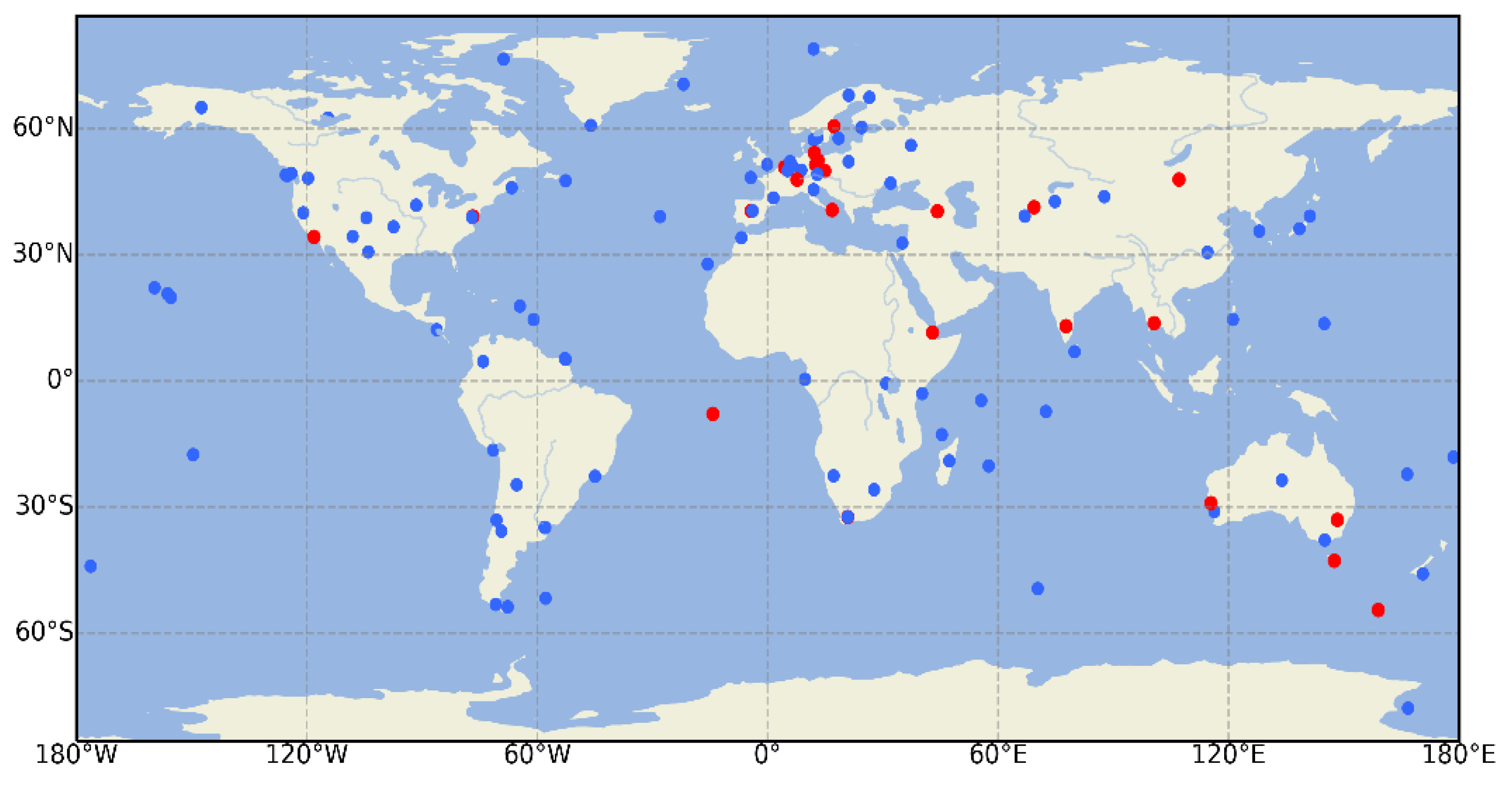
The previous theoretical analysis indicates that IFCBs stem from both the satellite- and receiver-dependent phase time-varying parts of the hardware delay, which is the difference between the satellite clock offsets for different IF combinations [25]. In this study, global data from 105 stations were collected for IFCB product estimation through methods considering different IF combinations. Subsequently, 25 stations were used to analyze the impact of IFCB stochastic modeling on the multi-GNSS multi-frequency PPP performance for simulated kinematic PPP. Based on the different IFCB processes, five schemes were implemented: (a) ignoring the effect of GPS third frequency IFCB, (b) using IFCB product correction, (c) using random constants to estimate the IFCB, (d) using a white noise process to estimate the IFCB, and (e) using a random walk process to estimate the IFCB. Then, the third-frequency residual was analyzed using the five schemes. The results are summarized and discussed after the analysis of the findings.

In this study, one-week observation data from 25 stations were used to evaluate PPP performance. The kinematic PPP performance was evaluated using indices such as positioning accuracy, convergence time, the third frequency phase residuals’ root mean square (RMS) and estimated IFCB. The position was considered to have converged only when the positioning error (east, north, up) of the epoch and the subsequent 20 epochs were within a 1 dm threshold [34,35]. For convenience, the five schemes mentioned above are marked as IFCB_NO (Neglect), IFCB_PC (Product Correction), IFCB_CT (random constant), IFCB_WN (white noise), and IFCB_RW (random walk), respectively. For the IFCB_RW scheme, the IFCB parameters were modeled as a random walk with a power density of 0.6 m/sqrt(s). The reason for using this value is explained in Section 4.1.2; for the first appearance of the satellite in the arc segment, the initial value of the IFCB was set to 0.01 m. It should be noted that the IFCB amplitudes of BDS-3 and Galileo are less than 2.0 cm, with negligible effects on multi-GNSS multi-frequency PPP positioning [4,14]; therefore, the effect of the third-frequency IFCB was ignored in this study. To facilitate the description, the IFCBs discussed in the following sections refer to the GPS L5 IFCB.

4.1. IFCB Estimation

4.1.1. IF Combinations Estimation (IFCB_PC)

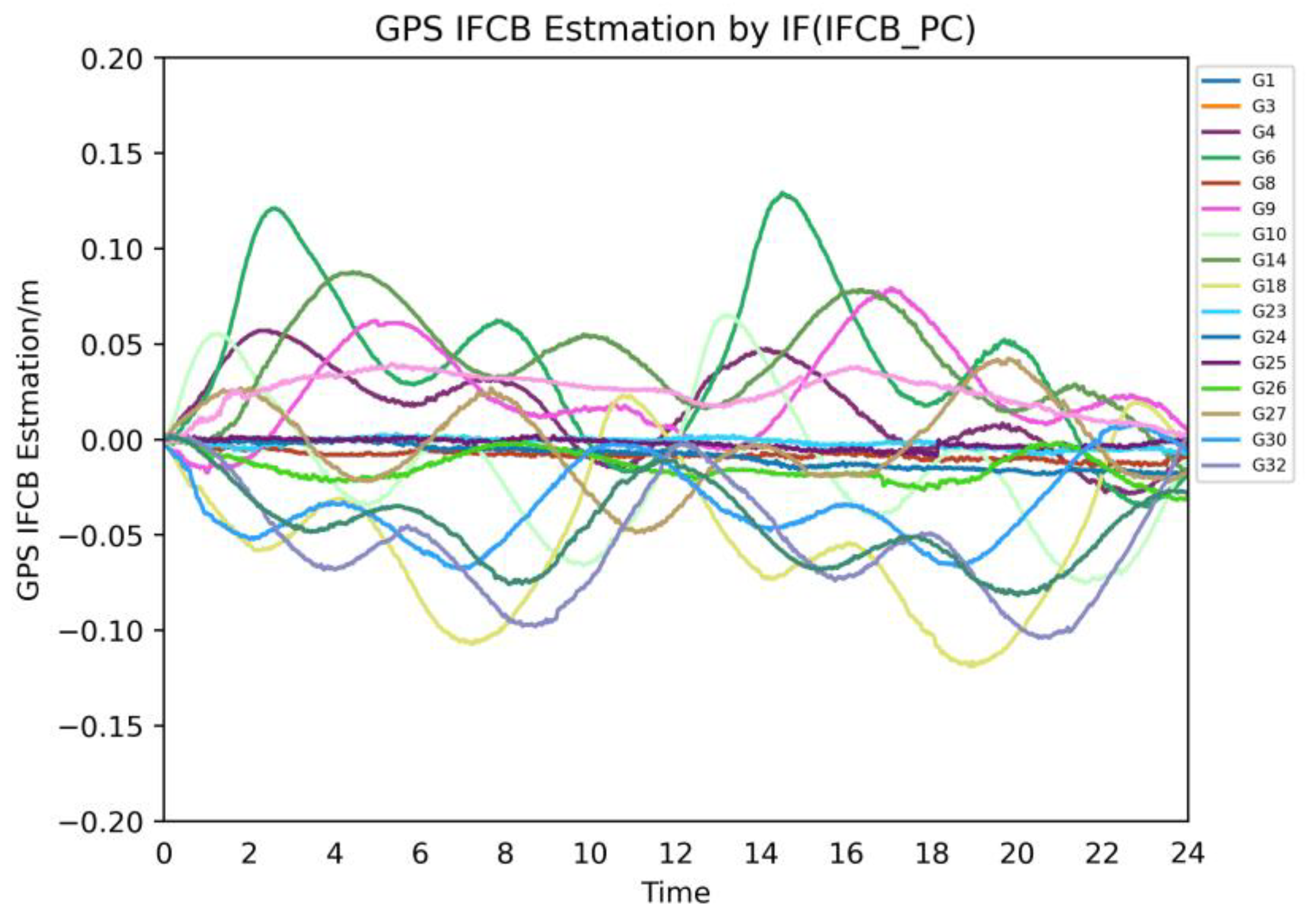
Figure 2 shows the GPS L5 IFCB products obtained using the IF combinations estimation, where different colors represent the IFCBs of different satellites. From Figure 2, the single-day amplitude of GPS Block IIF satellite L5 IFCB is larger among all satellites and lies within the range of 10–20 cm, which is obviously a PPP error that cannot be ignored. Additionally, it has been demonstrated that the amplitude of GPS Block III L5 IFCB ranges from 1 to 3 cm within a single day, and the standard deviation of IFCB is about 1.5 mm in a single epoch, which is almost independent of IFCB [4]. Therefore, it is necessary to focus only on the effect of the GPS Block IIF satellites’ L5 IFCB and to analyze the corresponding effect on the multi-GNSS multi-frequency PPP positioning (see Section 4.2). Since IFCB is considered a satellite- and receiver-related hardware delay between phase frequencies, which is caused by the difference between satellite clock offset calculated with different IF combinations, a thorough analysis of the satellite’s internal and external configuration is required to fully understand the causes of its generation. The focus of this study is on the impact of IFCB on multi-GNSS multi-frequency PPP positioning performance, so the causes of IFCB are not discussed in this paper.

4.1.2. Parameter Estimation (IFCB_CT, IFCB_WN, IFCB_RW)

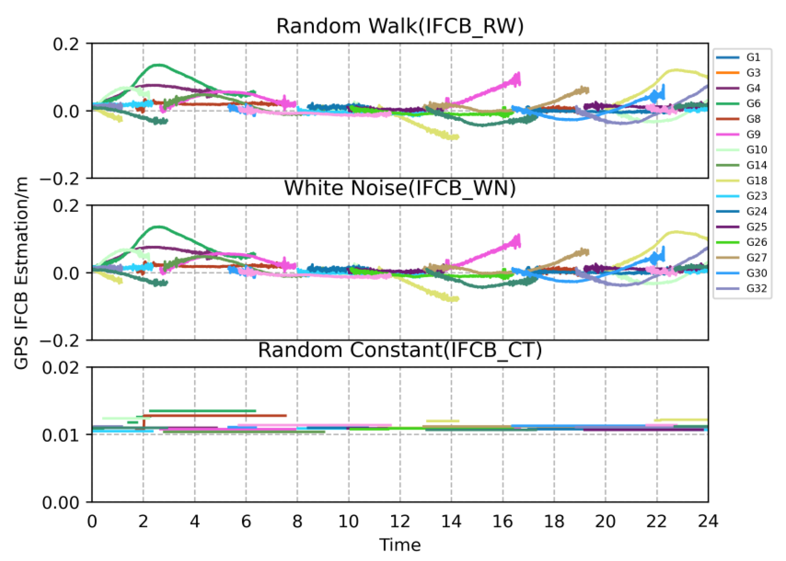
In order to analyze the effect of different stochastic models on IFCB results, in this section the IFCB is considered as a parameter and estimated lumped with other parameters, such as ambiguity, atmospheric error, and receiver clock offsets; corresponding time series are plotted. Taking BRUX station as an example, the IFCB daily series (DOY 18 January 2022) derived from the GPS/BDS-3 multi-GNSS multi-frequency PPP solutions are given in Figure 3, with different colors representing the IFCB of different satellites.

Figure 3 shows the IFCB results estimated via GPS/BDS-3 multi-frequency PPP using the IFCB_CT, IFCB_WN, and IFCB_RW schemes. It can be seen from

Table 2. IFCB amplitudes of GPS satellites (DOY 18 January 2022).

PRN	IFCB Amplitude/m
	IFCB_PC	IFCB_WN	IFCB_RW
G01	0.0860	0.0796	0.0795
G03	0.1660	0.1328	0.1328
G04	0.0150	0.0416	0.0413
G06	0.0980	0.0118	0.1175
G08	0.1410	0.1030	0.1029
G09	0.1050	0.0609	0.0608
G10	0.1420	0.2057	0.2056
G14	0.0130	0.0458	0.0415
G18	0.0200	0.0417	0.0427
G23	0.0110	0.0300	0.0314
G24	0.0340	0.0313	0.0313
G25	0.0920	0.0750	0.0749
G26	0.0770	0.1047	0.1046
G27	0.1070	0.1134	0.1133
G30	0.0430	0.0364	0.0364
G32	0.0840	0.0699	0.0699
AVG	0.0771	0.0740	0.0804
STD	0.0498	0.0492	0.0474

that the IFCB differences among the three IFCB process schemes (IFCB_PC, IFCB_WN, IFCB_RW) were less than 0.02 m for BRUX. Nonetheless, the IFCB differences between IFCB_CT and other schemes (IFCB_PC, IFCB_WN, and IFCB_RW) were significant. Comparing Figure 2 and Figure 3, in the IFCB_CT scheme, the estimation of IFCB as a random constant does not fit the characteristics of IFCB and cannot truly reflect the change of its temporal characteristics, thus affecting the positioning accuracy and convergence performance of the multi-GNSS multi-frequency PPP (see Section 4.2); therefore, the IFCB_CT scheme cannot be used to model IFCB variation.

The difference in satellite IFCB amplitudes between IFCB_PC and IFCB_WN was small, with an average difference of <1 cm, and the temporal characteristic change between them was similar, with an STD of <5 mm. Obviously, considering IFCB as a white noise process is consistent with the characteristic change of IFCB, which reflects the temporal characteristic change of IFCB more accurately and thus improves the multi-frequency PPP positioning accuracy and convergence. Therefore, the white noise process is suitable for describing the temporal characteristic change of IFCB. The same conclusion applies to the IFCB_RW scheme. It is worth noting that there are no studies on IFCB’s power spectral density (σ_IFCB) setting, so in order to obtain the optimal power spectral density value, the tests considered the range σ_IFCB $\in$ [60, 6 × 10⁻⁵] at the 25 stations (DOY 18 January 2022). The corresponding statistical results are shown in

Table 3. Determination experiment of GPS L5 IFCB power spectral density at 25 stations (DOY 18 January 2022).

${\mathit{\sigma }}_{\mathit{I}\mathit{F}\mathit{C}\mathit{B}}$ m/sqrt(s)		60	0.6	0.006	0.0006	0.00006
Convergence Time/min	AVERAGE	27.64			28.72	61.64
	MEDIAN	26.00			27.50	42.00

. As shown in Table 3, the convergence times in the σ_IFCB range within [60, 6 × 10⁻³] are equal, and the IFCB_PC results show that the inter-epoch variation and amplitude of IFCB are much smaller than 0.6 m, so σ_IFCB = 0.6 m/sqrt(s) is obviously a suitable choice for the IFCB_RW scheme. Consequently, this value was adopted chosen in this paper and the same value was used for the IFCB_WN scheme. The IFCB_WN scheme uses the same processing scheme as IFCB_RW. In conclusion, comparing Figure 2 and Figure 3 and the results in Table 2, IFCB_WN and IFCB_RW reflect the variation of the temporal characteristics of IFCB accurately, which indicates that the processing methods of the schemes used in this study are reasonable.

4.2. Three-Frequency PPP Performance

4.2.1. GPS-Only

The GPS-only results are given in Figure 4, which shows the convergence time box diagram for five IFCB process schemes. More than 24% of IFCB_CT schemes had a convergence time over 60 min; this performance was comparable with that of IFCB_NO. The average convergence times of the IFCB_RW and IFCB_WN schemes were comparable with that of IFCB_PC, with the difference being close to 1 min. The median convergence time improvement for the IFCB_RW and IFCB_WN schemes, compared to IFCB_NO was 43.0 min and 26.0 min, respectively. It is noteworthy that the convergence performance of GPS-Only PPP solutions was worst if the IFCB_NO or IFCB_CT schemes were adopted. This result was mostly caused by IFCB (see RMS values in

Table 4. RMS (m) of GPS-only PPP solutions among different IFCB process schemes at 25 stations for one week.

RMS/m						Improvement/%
IFCB	IFCB_NO	IFCB_PC	IFCB_CT	IFCB_WN	IFCB_RW	IFCB_PC	IFCB_CT	IFCB_WN	IFCB_RW
E	0.0512	0.0144	0.0229	0.0136	0.0136	71.9231	55.3678	73.3704	73.4434
N	0.0412	0.0123	0.0193	0.0117	0.0117	70.1304	53.2823	71.6625	71.6147
U	0.0601	0.0250	0.0345	0.0252	0.0252	58.4723	42.6752	57.9965	58.0559

).

Likewise, a clear difference in terms of weekly RMS was observed between the IFCB_NO scheme and the other four schemes (Table 4). The three IFCB process schemes (IFCB_PC, IFCB_WN, and IFCB_RW) were comparable in terms of positioning accuracy. Furthermore, the IFCB_NO and IFCB_CT schemes were generally worse than the other schemes.

4.2.2. GPS/BDS-3 and GPS/Galileo

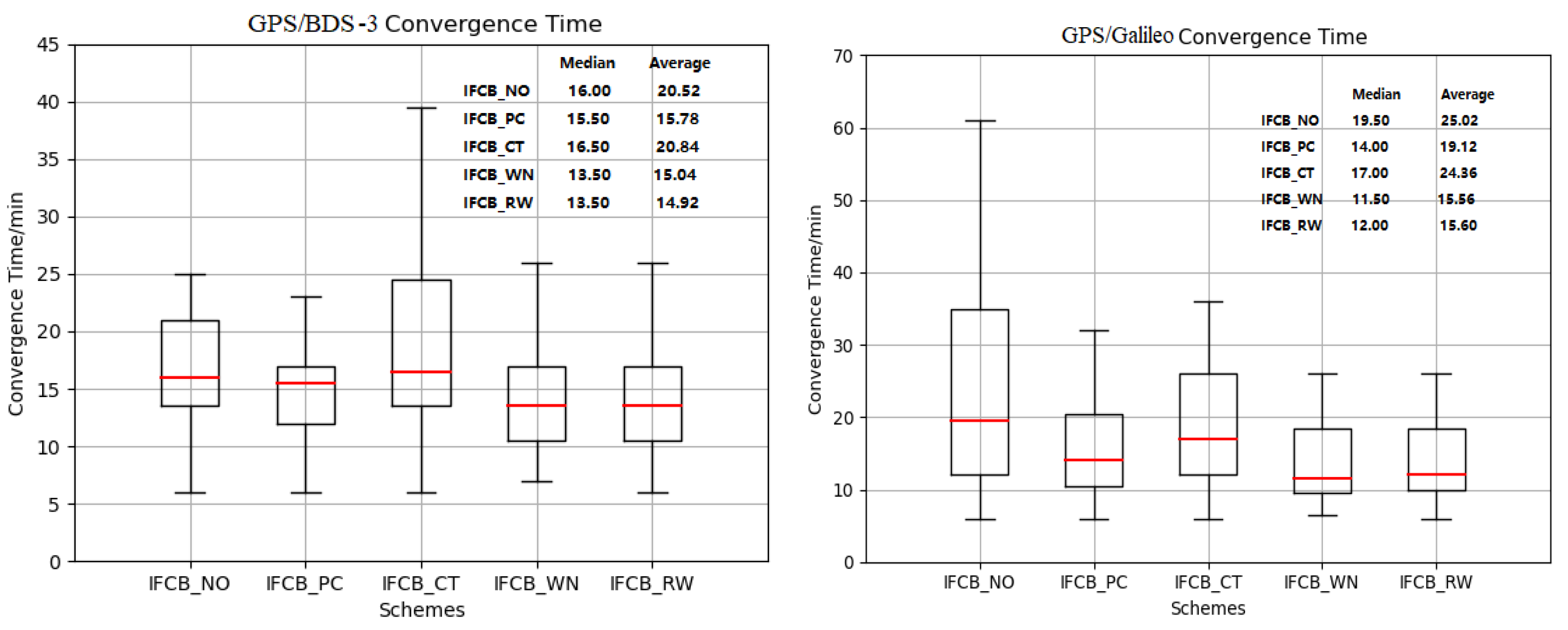
Figure 5 shows the convergence time box diagram of GPS/BDS-3 and GPS/Galileo PPP for the five IFCB process schemes. Similar to GPS-only, the convergence performance of the IFCB_PC, IFCB_RW, and IFCB_WN schemes (about 15 min on average for GPS/BDS-3) was much shorter than that of the IFCB_NO and IFCB_CT schemes (about 20 min on average for GPS/BDS-3), which is a striking improvement. In general, the convergence performance of the IFCB_PC, IFCB_RW, and IFCB_WN schemes is comparable. From Figure 6, it is evident that the GPS/Galileo convergence performance is similar to that of the GPS/BDS-3 PPP solutions.

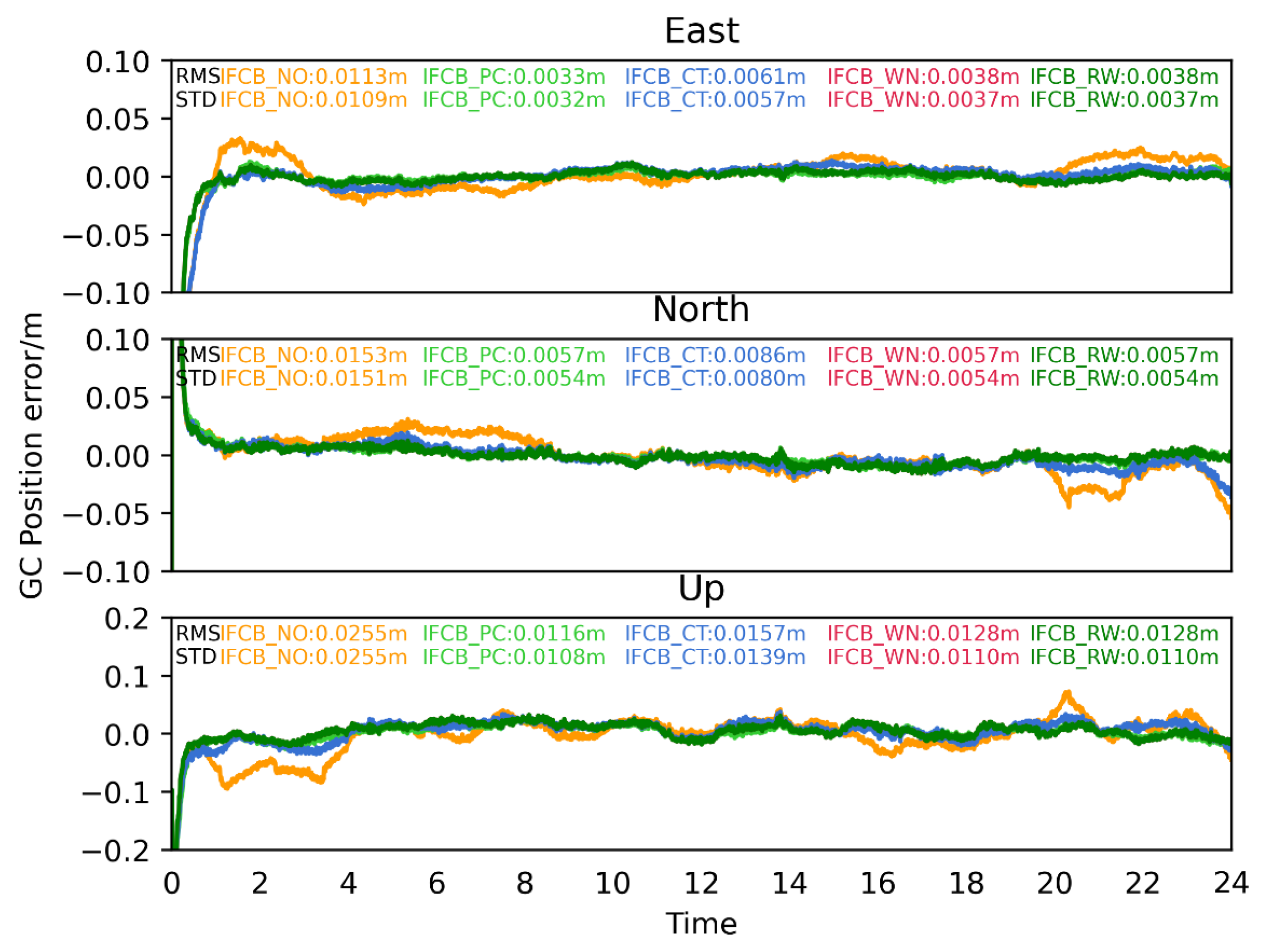
Figure 6 shows the comparisons of kinematic positioning errors for BRUX station for the five IFCB process schemes.

Table 5. RMS (m) of GPS/BDS-3 and GPS/Galileo PPP solutions among different IFCB process schemes at 25 stations for one week.

Mode	RMS/m						Improvement/%
	IFCB	IFCB_NO	IFCB_PC	IFCB_CT	IFCB_WN	IFCB_RW	IFCB_PC	IFCB_CT	IFCB_WN	IFCB_RW
GPS/BDS-3	E	0.0205	0.0100	0.0140	0.0101	0.0101	51.1308	31.6568	50.7240	50.7234
	N	0.0155	0.0095	0.0107	0.0093	0.0093	38.7091	30.8660	39.9950	39.9978
	U	0.0403	0.0197	0.0241	0.0190	0.0190	51.1071	40.1568	52.7273	52.7317
GPS/Galileo	E	0.0226	0.0102	0.0131	0.0094	0.0094	54.8057	41.8822	58.5311	58.5279
	N	0.0164	0.0094	0.0106	0.0089	0.0089	42.5375	35.0849	45.3270	45.3292
	U	0.0374	0.0211	0.0246	0.0205	0.0205	43.4080	34.2153	45.0044	45.0119

shows the weekly positioning accuracy of GPS/BDS-3 PPP at the 25 stations for the five IFCB schemes. Not surprisingly, the positioning accuracy of the IFCB_NO scheme is worse than that of the other schemes. Comparing IFCB_NO with the other three schemes (IFCB_PC, IFCB_WN, and IFCB_RW), the positioning accuracy is improved by 50.72% (from 2.05 cm to 1.01 cm) in the east, by 39.99% (1.55 cm to 0.93 cm) in the north, and by 52.72% (4.03 cm to 1.90 cm) in the up components. As shown in Table 5, the positioning accuracy of the multi-GNSS multi-frequency PPP solutions with IFCB_PC, IFCB_WN, and IFCB_RW is comparable among the five IFCB process schemes.

With regard to convergence as GPS/Galileo PPP solutions, one can see from Table 5 that the positioning accuracy of the IFCB_PC, IFCB_RW, and IFCB_WN schemes is improved by 58.53% (from 2.26 cm to 0.94 cm) in the east, 45.33% (1.64 cm to 0.89 cm) in the north, and by 45.00% (3.74 cm to 2.05 cm) in the up components compared with the IFCB_NO scheme. As shown in Table 5, the IFCB_PC, IFCB_WN, and IFCB_RW schemes are comparable among the five IFCB process schemes for positioning accuracy of PPP solutions.

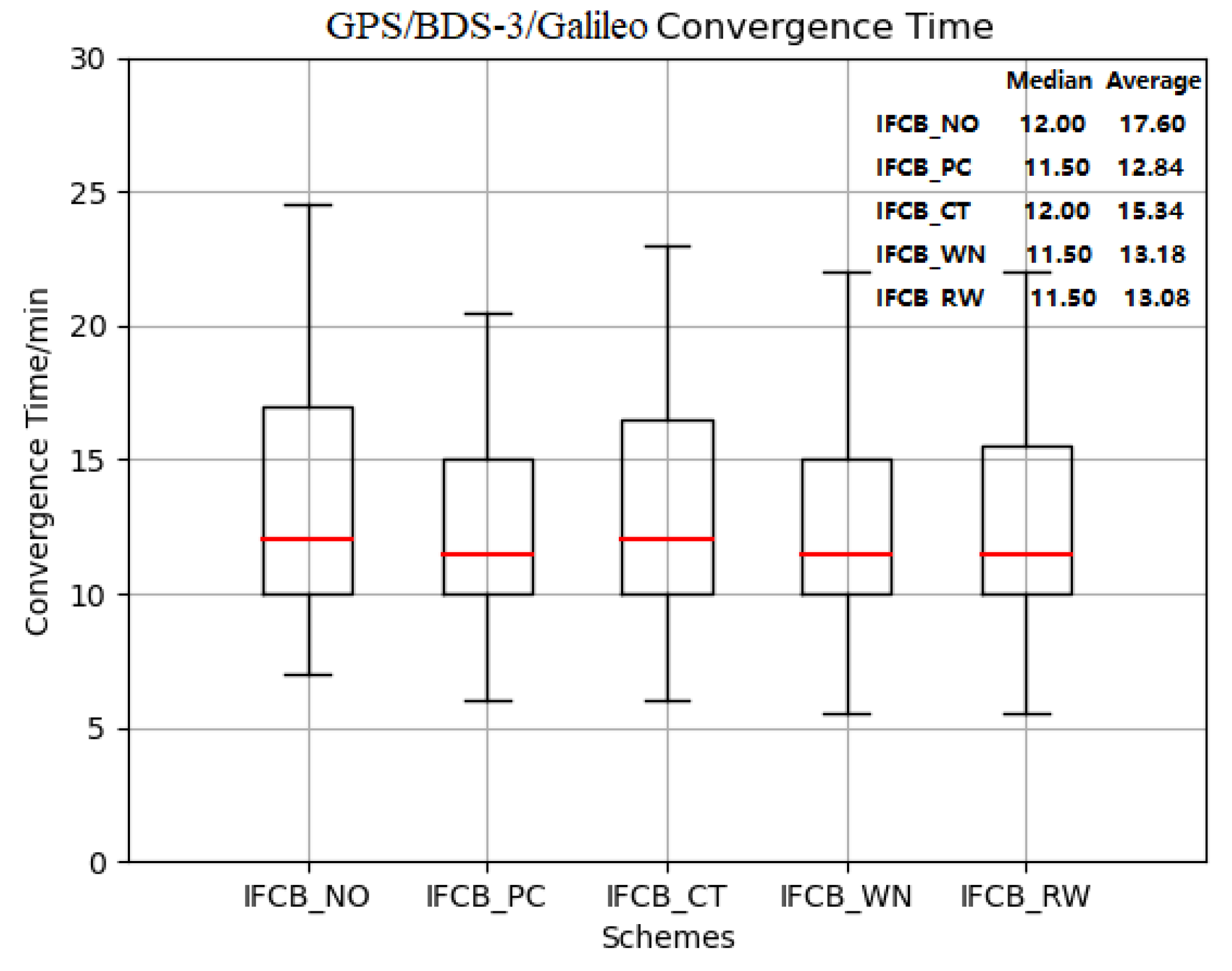
4.2.3. GPS/BDS-3/Galileo

Figure 7 shows the convergence time box diagram of GPS/BDS-3/Galileo PPP for the five IFCB process schemes. It is evident that the differences in convergence performance are similar to those of the GPS/BDS-3 PPP solutions.

Comparing IFCB_PC, IFCB_WN, and IFCB_RW convergence times of GPS/BDS-3/Galileo PPP solutions, the average convergence time of IFCB_NO (or IFCB_CT) is 5 min less than that of IFCB_WN (and IFCB_PC or IFCB_RW). It is also evident, from Figure 7, that the median convergence times are comparable among the five IFCB process schemes. This is attributed to the increase in the number of BDS-3 and Galileo observations, in which the strength of the observation equation and the redundancy are increased. The positioning accuracy of the IFCB_PC, IFCB_RW, and IFCB_WN schemes is improved by 41.34% (from 1.37 cm to 0.81 cm) in the east, by 23.29% (1.10 cm to 0.84 cm) in the north, and by 37.92% (2.72 cm to 1.70 cm) in the up components compared to the IFCB_NO scheme. As shown in

Table 6. RMS (m) of GPS/BDS-3/Galileo PPP solutions among the five IFCB process schemes at the 25 stations over one week.

RMS/m						Improvement/%
IFCB	IFCB_NO	IFCB_PC	IFCB_CT	IFCB_WN	IFCB_RW	IFCB_PC	IFCB_CT	IFCB_WN	IFCB_RW
E	0.0137	0.0082	0.0098	0.0081	0.0080	40.2152	28.6915	41.3393	41.7205
N	0.0110	0.0084	0.0087	0.0083	0.0083	23.2906	20.8129	24.0852	24.2910
U	0.0272	0.0175	0.0195	0.0169	0.0169	35.6965	28.2565	37.9158	37.9304

, the IFCB_PC, IFCB_WN, and IFCB_RW schemes are comparable among the five IFCB process schemes for positioning accuracy of PPP solutions.

In conclusion, the above three sets of experiments show that it is feasible to use the parameter estimation method to deal with IFCB, and its effect on positioning accuracy and convergence performance is comparable to that of using product correction. Therefore, the white noise or random walk process can be used to describe IFCB parameters to accelerate the multi-GNSS multi-frequency PPP convergence in the absence of product correction or real-time applications.

4.3. Residual Analysis

Some unmodeled errors, such as IFCB, are reflected in the post residuals due to poor observation models or incomplete corrections. Figure 8 shows the post-phase residuals of the five IFCB process schemes of GPS L5 at BRUX station (DOY 18 January 2022), where different colors represent the residuals of different satellites. As previously concluded, the IFCB_NO and IFCB_CT schemes exhibit significant systematic bias effects in the GPS L5 phase residuals, while the IFCB_PC, IFCB_WN, and IFCB_RW schemes eliminate these effects. 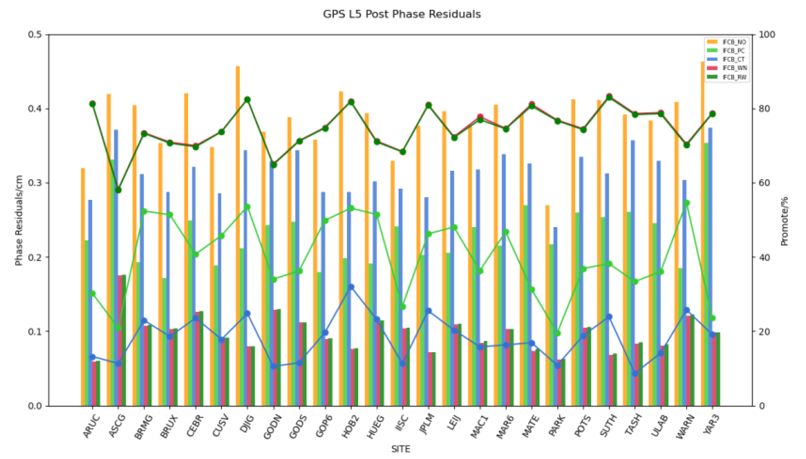At the same time, to further evaluate the effect of IFCB on GPS L5 phase residuals, Figure 9 and

Table 7. RMS (cm) of GPS PPP L5 phase residuals among different IFCB process schemes at the 25 stations over one week.

RMS/cm					Promote/%
IFCB_NO	IFCB_PC	IFCB_CT	IFCB_WN	IFCB_RW	IFCB_PC	IFCB_CT	IFCB_WN	IFCB_RW
0.3867	0.2311	0.3148	0.0971	0.0980	40.25	18.60	74.89	74.66

give the weekly RMS values of the GPS L5 phase residuals for the 25 stations. The histogram in Figure 9 shows the average GPS L5 phase residuals for one week at the 25 stations, while the line graph shows the percentage improvement of each station relative to the IFCB_NO scheme. Table 7 shows the average GPS L5 phase residual RMS values over one week of the five process schemes at the 25 stations. Compared to IFCB_NO, the RMS of the GPS L5 phase residuals of IFCB_PC, IFCB_WN, and IFCB_RW were improved from 0.3867 cm to 0.2311 cm, 0.0971 cm, and 0.0980 cm, respectively, which represent improvements of 40.25%, 74.89%, and 74.66%. The effect is especially pronounced in the case of the IFCB_WN and IFCB_RW schemes. Accordingly, it is concluded that the effect of the apparent systematic bias in the GPS L5 phase residuals can be eliminated using the IFCB_PC, IFCB_WN, or IFCB_RW schemes; the latter two schemes have significantly better residual values than the IFCB_PC scheme. The above conclusions indicate that the use of the estimation method results in an improved correction of the effects of IFCB compared to the use of product correction, and can help avoid satellite false rejects due to large residuals during data processing.

4.4. Discussion

The above results show that ignoring the effect of IFCB can seriously degrade the positioning performance of multi-GNSS multi-frequency PPP, and therefore the effect of IFCB must be considered. The IF combinations’ IFCB estimation method averages the IFCB over all stations, and although this method uses epoch differences in the calculation process to eliminate most of the errors, there are still some unmodeled errors remaining in the epoch-difference GFIF observations, such as multipath, higher-order ionospheric delay, and others. This method does not consider the receiver IFCB, so the average receiver IFCB is absorbed by the satellite IFCB. If the number of stations in the network is limited, the receiver IFCB cannot be eliminated through averaging, so this method is not theoretically rigorous [25]. This is also the reason why the residuals of IFCB_PC are larger than those of IFCB_RW or IFCB_WN. This effect can be derived from the following equation:

Taking into account the unmodeled error ${\tau }_r^s$ in Equation (10), the following equation can be obtained:

$$GFIF=L_{r,IF12}^s-L_{r,IF13}^s=N_{GFIF}+B_{r,GFIF}^s+\delta \hat{B}+{\tau }_r^s$$

(18)

Then, the new epoch-difference GFIF is expressed as follows:

$$GFI{F}_t-GFI{F}_{t-1}=\mathsf{\Delta }\delta {\hat{B}}_{(t,t-1)}+{\tau }_{r,(t,t-1)}^s$$

(19)

Therefore, the current epoch satellite IFCB becomes:

$$\mathsf{\Delta }\delta {\overline{B}}_{(t,t-1)}=\frac{{\displaystyle \sum _{r=1}^n(\mathsf{\Delta }\delta {\hat{B}}_{(t,t-1)}+{\tau }_{r,(t,t-1)}^s)·{\omega }_{r,(t,t-1)}}}{{\displaystyle \sum _{r=1}^n{\omega }_{r,(t,t-1)}}}$$

(20)

Obviously ${\tau }_{r,(t,t-1)}^s$ causes an accumulation of errors, indicating that the IFCB estimated using the IFCB_PC method contains an unmodeled error ${\tau }_r^s$ for n stations, but this unmodeled error is small (RMS < 2 mm, see RMS values in Table 7) and can be neglected. The analysis in the previous sections shows that IFCB_NO and IFCB_CT have comparable convergence performance, but the positioning accuracy of the latter is improved. IFCB_PC has comparable positioning accuracy and convergence time with IFCB_WN and IFCB_RW, but the residuals of the latter two are smaller than that of the former. This indicates that the use of a proper IFCB stochastic model can achieve comparable performance with the use of the product, but the method of IFCB parameter estimation increases the computational effort on the user side and incurs higher requirements for user equipment. However, the impact on positioning performance is minimal. Therefore, the IFCB_RW or IFCB_WN methods are recommended for processing IFCB, when an IFCB product is unavailable, in the case of users requiring real-time applications.

5. Conclusions

The incorporation of multi-frequency signals into GNSS has introduced new possibilities for precise positioning and rapid ambiguity resolution. The IFCB pertains to the variation in clock offsets among distinct frequencies of satellite signals, and its proper processing is of great importance, as it significantly impacts PPP accuracy when using multi-frequency signals. Neglecting the IFCB can result in reduced positioning accuracy and increased convergence time in both static and kinematic PPP solutions. In this study, the focus lies on the appropriate modeling for phase IFCB in multi-GNSS multi-frequency PPP based on the UDUC observation model. The optimal power spectral density applicable to IFCB is analyzed and studied, and the product correction methods are compared with parameter estimation methods. The impact of IFCB stochastic modeling on the performance of Undifferenced and Uncombined PPP is also evaluated from the aspects of convergence time and positioning accuracy through five IFCB process schemes, namely IFCB_NO, IFCB_PC, IFCB_CT, IFCB_RW, and IFCB_WN.

To validate these findings, an analysis of the effect of IFCB stochastic modeling on UDUC the multi-GNSS multi-frequency PPP performance was conducted using weekly data (DOY 18–24 January 2022) from 130 IGS MGEX tracking stations. Through this analysis, the following conclusions can be stated: (i) the optimal power spectral density for IFCB is 60, 0.006 m/sqrt(s); (ii) modeling IFCB as a random walk is feasible; (iii) the multi-GNSS multi-frequency PPP performance is comparable and best for the IFCB_PC, IFCB_RW, and IFCB_WN schemes, while the performance of the IFCB_NO and IFCB_CT schemes is poor; (iv) the third frequency phase residuals of the IFCB_RW and IFCB_WN scheme are smaller than those of the IFCB_PC scheme. However, any potential impacts on the troposphere, ionosphere, and float ambiguity are not discussed.

The methodology for estimating multi-GNSS satellite phase products is currently in a developmental stage, thus these products are not yet fully mature. The commonly utilized approach, which involves the use of IFCBs corrected via products, is applicable exclusively when the server provides such products. However, IFCB products are not readily accessible, especially for users who require immediate and continuous positioning solutions. Essentially, a random walk is an expansion and accumulation of white noise, and the IFCB_RW and IFCB_WN schemes are indistinguishable. However, compared to white noise, the random walk has the advantages of exhibiting trends, correlation, and memory, making it more suitable for modeling phenomena with directionality, time dependence, and historical dependence. Therefore, in the absence of IFCB products, modeling IFCBs as random walks can result in significantly more reliable performance.

References

1. Hein, G.W. Status, perspectives and trends of satellite navigation. Satell. Navig. 2020, 1, 22. [Google Scholar] [CrossRef] [PubMed]
2. Montenbruck, O.; Hauschild, A.; Steigenberger, P.; Langley, R. Three’s the Challenge: A Close Look at GPS SVN62 Triple-frequency Signal Combinations Finds Carrier-phase Variations on the New L5. GPS World 2010, 21, 8–19. [Google Scholar]
3. Pan, L.; Zhang, X.; Guo, F.; Liu, J. GPS inter-frequency clock bias estimation for both uncombined and ionospheric-free combined triple-frequency precise point positioning. J. Geod. 2019, 93, 473–487. [Google Scholar] [CrossRef]
4. Pan, L.; Li, X.; Zhang, X.; Li, X.; Lu, C.; Zhao, Q.; Liu, J. Considering Inter-Frequency Clock Bias for BDS Triple-Frequency Precise Point Positioning. Remote Sens. 2017, 9, 734. [Google Scholar] [CrossRef]
5. Guo, J.; Geng, J. GPS satellite clock determination in case of inter-frequency clock biases for triple-frequency precise point positioning. J. Geod. 2018, 92, 1133–1142. [Google Scholar] [CrossRef]
6. Montenbruck, O.; Hugentobler, U.; Dach, R.; Steigenberger, P.; Hauschild, A. Apparent clock variations of the Block IIF-1 (SVN62) GPS satellite. GPS Solut. 2012, 16, 303–313. [Google Scholar] [CrossRef]
7. Li, H.; Li, B.; Xiao, G.; Wang, J.; Xu, T. Improved method for estimating the inter-frequency satellite clock bias of triple-frequency GPS. GPS Solut. 2016, 20, 751–760. [Google Scholar] [CrossRef]
8. Li, H.; Zhou, X.; Wu, B.; Wang, J. Estimation of the inter-frequency clock bias for the satellites of PRN25 and PRN01. Sci. China-Phys. Mech. Astron. 2012, 55, 2186–2193. [Google Scholar] [CrossRef]
9. Wang, Z.; Wang, R.; Wang, Y.; Hu, C.; Liu, B. Modelling and Assessment of a New Triple-Frequency IF1213 PPP with BDS/GPS. Remote Sens. 2022, 14, 4509. [Google Scholar] [CrossRef]
10. Li, X.; Li, X.; Liu, G.; Feng, G.; Yuan, Y.; Zhang, K.; Ren, X. Triple-frequency PPP ambiguity resolution with multi-constellation GNSS: BDS and Galileo. J. Geod. 2019, 93, 1105–1122. [Google Scholar] [CrossRef]
11. Xu, G.; Xu, Y. Applications of GPS theory and algorithms. In GPS; Springer: Berlin/Heidelberg, Germany, 2016. [Google Scholar]
12. Xie, X.; Fang, R.; Geng, T.; Wang, G.; Zhao, Q.; Liu, J. Characterization of GNSS Signals Tracked by the iGMAS Network Considering Recent BDS-3 Satellites. Remote Sens. 2018, 10, 1736. [Google Scholar] [CrossRef]
13. Zhang, F.; Chai, H.; Li, L.; Xiao, G.; Du, Z. Estimation and analysis of GPS inter-fequency clock biases from long-term triple-frequency observations. GPS Solut. 2021, 25, 126. [Google Scholar] [CrossRef]
14. Pan, L.; Zhang, X.; Li, X.; Liu, J.; Li, X. Characteristics of inter-frequency clock bias for Block IIF satellites and its effect on triple-frequency GPS precise point positioning. GPS Solut. 2017, 21, 811–822. [Google Scholar] [CrossRef]
15. Li, H.; Zhou, X.; Wu, B. Fast estimation and analysis of the inter-frequency clock bias for Block IIF satellites. GPS Solut. 2013, 17, 347–355. [Google Scholar] [CrossRef]
16. Fan, L.; Shi, C.; Li, M.; Wang, C.; Zheng, F.; Jing, G.; Zhang, J. GPS satellite inter-frequency clock bias estimation using triple-frequency raw observations. J. Geod. 2019, 93, 2465–2479. [Google Scholar] [CrossRef]
17. Thoelert, S.; Steigenberger, P.; Montenbruck, O. Signal analysis of the first GPS III satellite. GPS Solut. 2019, 23, 92. [Google Scholar] [CrossRef]
18. Chen, Y.; Mi, J.; Gu, S.; Li, B.; Li, H.; Yang, L.; Pang, Y. GPS, BDS-3, and Galileo Inter-Frequency Clock Bias Deviation Time-Varying Characteristics and Positioning Performance Analysis. Remote Sens. 2022, 14, 3991. [Google Scholar] [CrossRef]
19. Zhang, Z.; Pan, L. Modeling and predicting inter-frequency clock bias of BDS-2 GEO, IGSO and MEO satellites for triple-frequency precise point positioning. GPS Solut. 2022, 26, 89. [Google Scholar] [CrossRef]
20. Gong, X.; Gu, S.; Lou, Y.; Zheng, F.; Yang, X.; Wang, Z.; Liu, J. Research on empirical correction models of GPS Block IIF and BDS satellite inter-frequency clock bias. J. Geod. 2020, 94. [Google Scholar] [CrossRef]
21. Li, P.; Jiang, X.; Zhang, X.; Ge, M.; Schuh, H. GPS + Galileo + BeiDou precise point positioning with triple-frequency ambiguity resolution. GPS Solut. 2020, 24, 78. [Google Scholar] [CrossRef]
22. Geng, J.; Guo, J.; Meng, X.; Gao, K. Speeding up PPP ambiguity resolution using triple-frequency GPS/BeiDou/Galileo/QZSS data. J. Geod. 2020, 94, 6. [Google Scholar] [CrossRef]
23. Guo, F.; Zhang, X.; Wang, J.; Ren, X. Modeling and assessment of triple-frequency BDS precise point positioning. J. Geod. 2016, 90, 1223–1235. [Google Scholar] [CrossRef]
24. Xiang, Y.; Gao, Y.; Shi, J.; Xu, C. Carrier phase-based ionospheric observables using PPP models. Geod. Geodyn. 2017, 8, 17–23. [Google Scholar] [CrossRef]
25. Zhang, Y.; Nobuaki, K.; Chen, J.; Wang, H.; Wang, J. An improved method for BDS inter-frequency clock bias estimation. In Proceedings of the China Satellite Navigation Conference (CSNC), Beijing, China, 22–25 May 2019; Volume II. [Google Scholar]
26. Kouba, J. A Guide to Using International GNSS Service (IGS) Products; Geodetic Survey Division; Natural Resources Canada: Ottawa, ON, Canada, 2015.
27. Liu, T.; Zhang, B.; Yuan, Y.; Li, Z.; Wang, N. Multi-GNSS triple-frequency differential code bias (DCB) determination with precise point positioning (PPP). J. Geod. 2018, 93, 765–784. [Google Scholar] [CrossRef]
28. Zhang, B.; Teunissen, P.J.; Yuan, Y. On the short-term temporal variations of GNSS receiver differential phase biases. J. Geod. 2017, 91, 563–572. [Google Scholar] [CrossRef]
29. Rebischung, P.; Schmid, R. IGS14/igs14.atx: A new framework for the IGS products. In Proceedings of the AGU Fall Meeting, San Francisco, CA, USA, 10–14 December 2017. [Google Scholar]
30. Li, X.; Ge, M.; Dai, X.; Ren, X.; Fritsche, M.; Wickert, J.; Schuh, H. Accuracy and reliability of multi-GNSS real-time precise positioning: GPS, GLONASS, BeiDou, and Galileo. J. Geod. 2015, 89, 607–635. [Google Scholar] [CrossRef]
31. Li, P.; Zhang, X. Integrating GPS and GLONASS to accelerate convergence and initialization times of precise point positioning. GPS Solut. 2014, 18, 461–471. [Google Scholar] [CrossRef]
32. Zhou, F.; Dong, D.; Li, W.; Jiang, X.; Wickert, J.; Schuh, H. GAMP: An open-source software of multi-GNSS precise point positioning using undifferenced and uncombined observations. GPS Solut. 2018, 22, 33. [Google Scholar] [CrossRef]
33. Zhou, F.; Dong, D.; Li, P.; Li, X.; Schuh, H. Influence of stochastic modeling for inter-system biases on multi-GNSS undifferenced and uncombined precise point positioning. GPS Solut. 2019, 23, 59. [Google Scholar] [CrossRef]
34. Li, B.; Mi, J.; Zhu, H.; Gu, S.; Xu, Y.; Wang, H.; Yang, L.; Chen, Y.; Pang, Y. BDS-3/GPS/Galileo OSB Estimation and PPP-AR Posi-tioning Analysis of Different Positioning Models. Remote Sens. 2022, 14, 4207. [Google Scholar] [CrossRef]
35. Lou, Y.; Zheng, F.; Gu, S.; Wang, C.; Guo, H.; Feng, Y. Multi-GNSS precise point positioning with raw single-frequency and dual-frequency measurement models. GPS Solut. 2016, 20, 849–862. [Google Scholar] [CrossRef]
Figure 1. MGEX stations used in the experiment. Blue dots represent stations used to estimate IFCB by IF; red dots represent stations used for PPP validation.
Remotesensing 15 04507 g001
Figure 2. GPS L5 IFCB based on the combined IF observations of 105 stations (DOY 18 January 2022), where each color represents a satellite.
Remotesensing 15 04507 g002
Figure 3. GPS IFCB for BRUX station based on the IFCB process Schemes IFCB_RW, IFCB_WN and IFCB_CT (DOY 18 January 2022), where each color represents a satellite.
Remotesensing 15 04507 g003
Figure 4. Comparisons of GPS-only convergence times for the five IFCB process schemes over 7 days.
Remotesensing 15 04507 g004
Figure 5. Comparisons of GPS/BDS-3 (Left) and GPS/Galileo (Right) convergence times for the five IFCB process schemes over 7 days.
Remotesensing 15 04507 g005
Figure 6. Comparisons of kinematic positioning errors for BRUX station for the five IFCB process schemes (DOY 18 January 2022).
Remotesensing 15 04507 g006
Figure 7. Comparisons of GPS/BDS-3/Galileo convergence times for the five IFCB process schemes over 7 days.
Remotesensing 15 04507 g007
Figure 8. Comparisons of GPS L5 post phase residuals for BRUX station based on the five IFCB process schemes (DOY 18 January 2022), where each color represents a satellite.
Remotesensing 15 04507 g008
Figure 9. RMS error of GPS L5 phase residuals for the 25 stations over 7 days (RMS, unit: cm).
Remotesensing 15 04507 g009