Author Contributions
Conceptualization, Z.Z., E.L. and Z.M.; Methodology, Z.Z.; Software, Z.Z.; Validation, Z.Z.; Formal analysis, A.Z.; Supervision, M.Q.-H.M.; Project administration, Y.Y. All authors have read and agreed to the published version of the manuscript.
Figure 1.
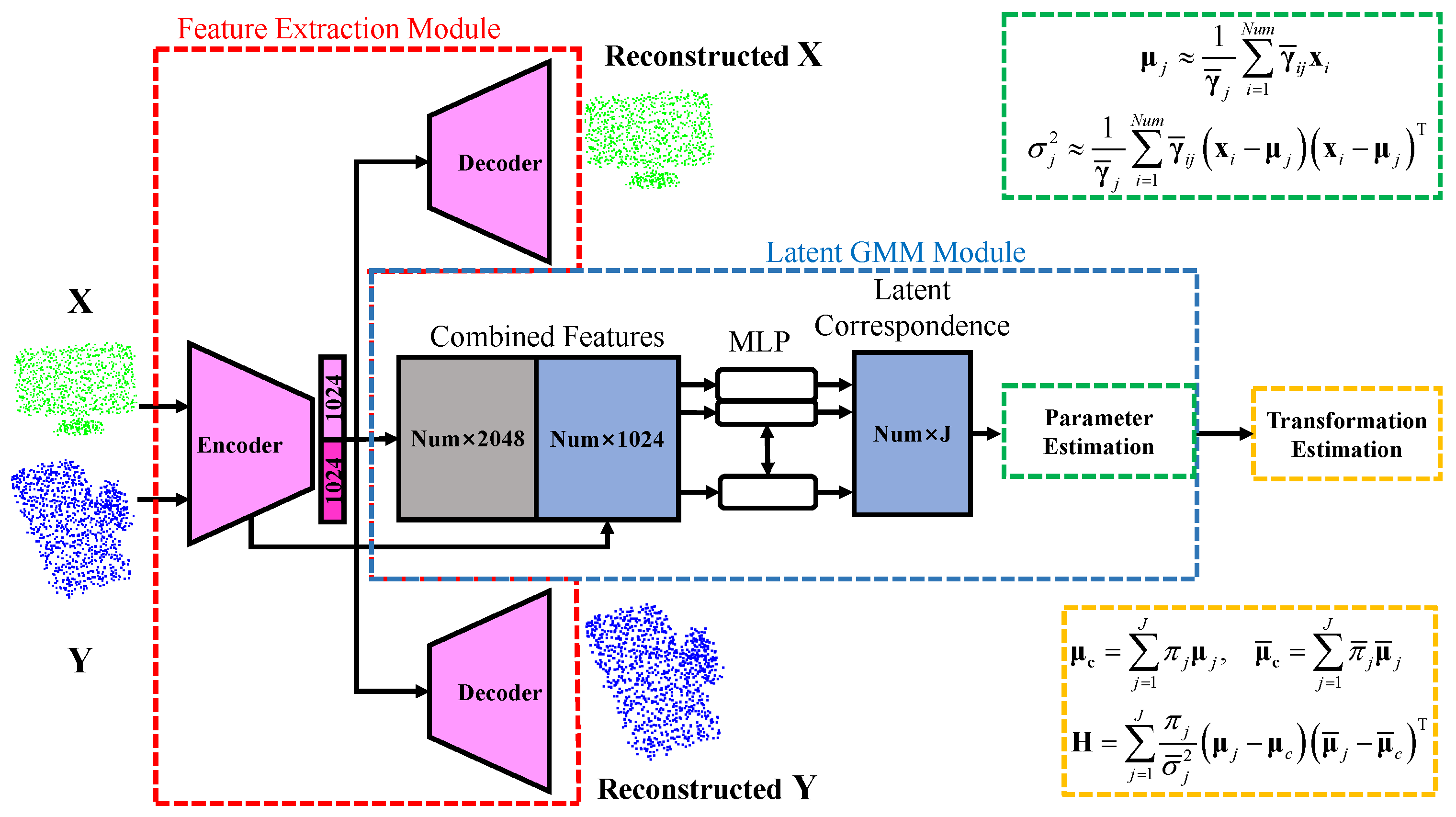
The overview of the proposed PCR method. The equations denoted by the green dashed line are used to estimate the latent source GMM component, while the equations denoted by the orange dashed line in the lower right corner are used in the weighted SVD module.
Figure 1.
The overview of the proposed PCR method. The equations denoted by the green dashed line are used to estimate the latent source GMM component, while the equations denoted by the orange dashed line in the lower right corner are used in the weighted SVD module.
Figure 2.
The architecture of the proposed autoencoder module.
Figure 2.
The architecture of the proposed autoencoder module.
Figure 3.
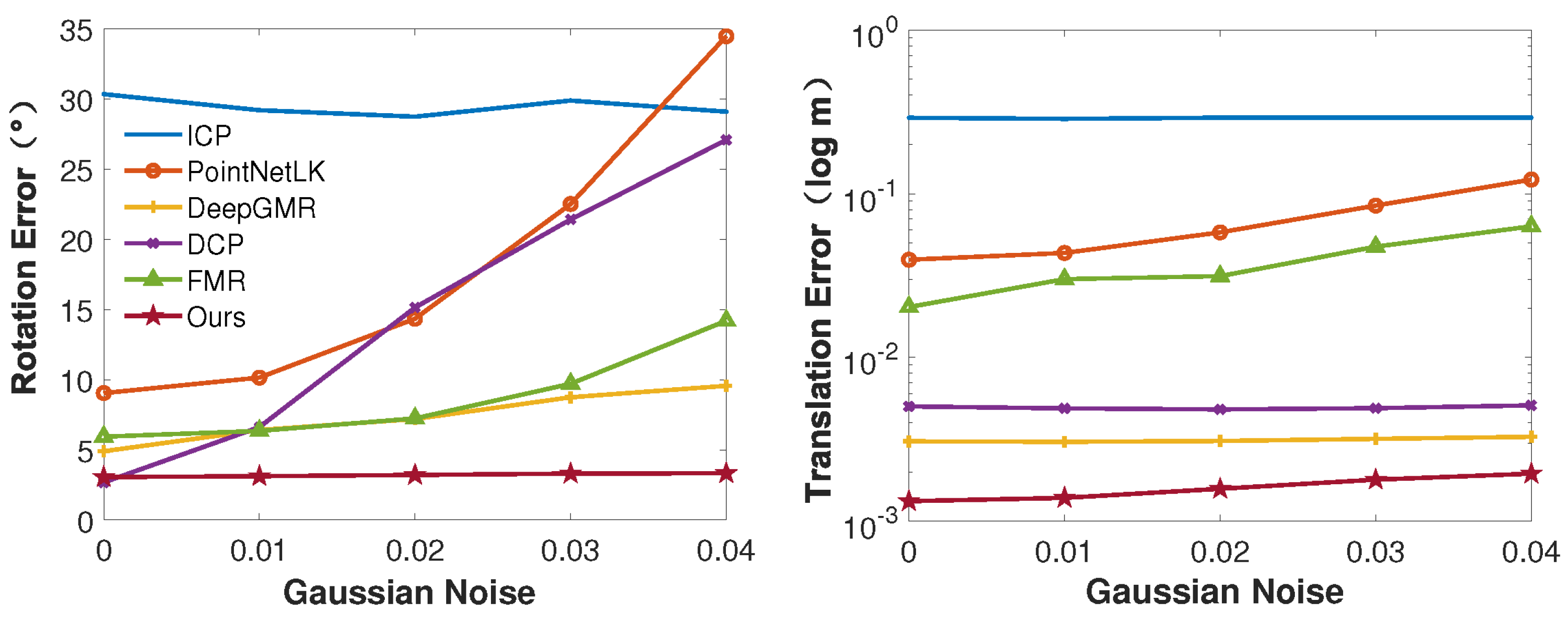
Comparison results on the noisy dataset. Even when noise is relative large ( 0.04), the proposed method achieves accurate and robust performances.
Figure 3.
Comparison results on the noisy dataset. Even when noise is relative large ( 0.04), the proposed method achieves accurate and robust performances.
Figure 4.
Qualitative registration results on the noisy ModelNet40 dataset (). The figures in three rows show the registration results of three classes of objects, including person, stool, and toilet. The source and target point cloud are shown in green and blue, respectively.
Figure 4.
Qualitative registration results on the noisy ModelNet40 dataset (). The figures in three rows show the registration results of three classes of objects, including person, stool, and toilet. The source and target point cloud are shown in green and blue, respectively.
Figure 5.
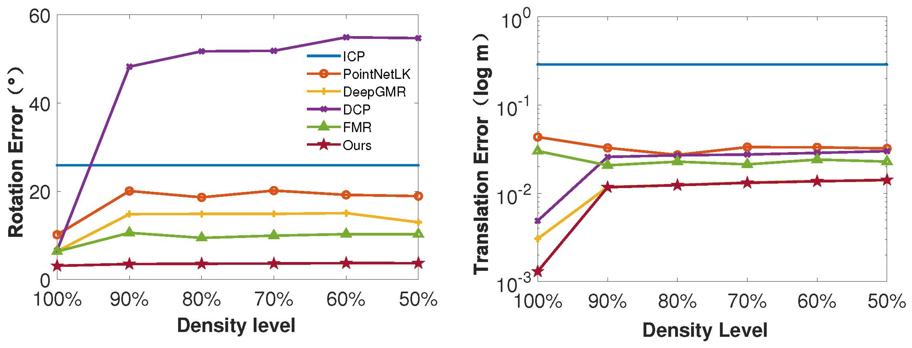
Comparison results on different density levels. The results confirm that our algorithm consistently exhibits accuracy and robustness in sparse PCR experiments.
Figure 5.
Comparison results on different density levels. The results confirm that our algorithm consistently exhibits accuracy and robustness in sparse PCR experiments.
Figure 6.
Qualitative registration results on noisy ModelNet40 dataset (). Figures in two rows show the registration results of two classes of objects, including wardrobe and table. The results show that our algorithm has better robustness to the used sparse data.
Figure 6.
Qualitative registration results on noisy ModelNet40 dataset (). Figures in two rows show the registration results of two classes of objects, including wardrobe and table. The results show that our algorithm has better robustness to the used sparse data.
Figure 7.
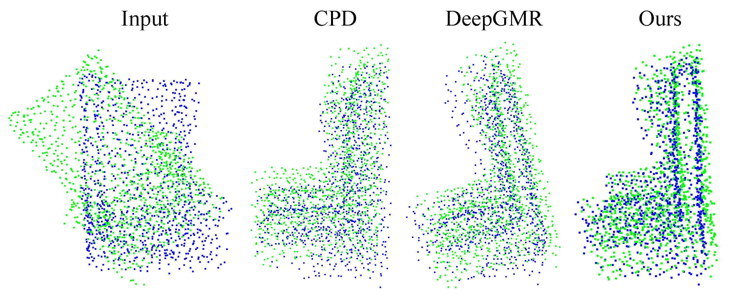
Qualitative registration results on partial data. The figures show the registration results of CPD, DeepGMR, and ours.
Figure 7.
Qualitative registration results on partial data. The figures show the registration results of CPD, DeepGMR, and ours.
Figure 8.
Qualitative registration results on the real-world dataset. Figures in two rows show the registration results of two classes of scenes, including the kitchen and office.
Figure 8.
Qualitative registration results on the real-world dataset. Figures in two rows show the registration results of two classes of scenes, including the kitchen and office.
Figure 9.
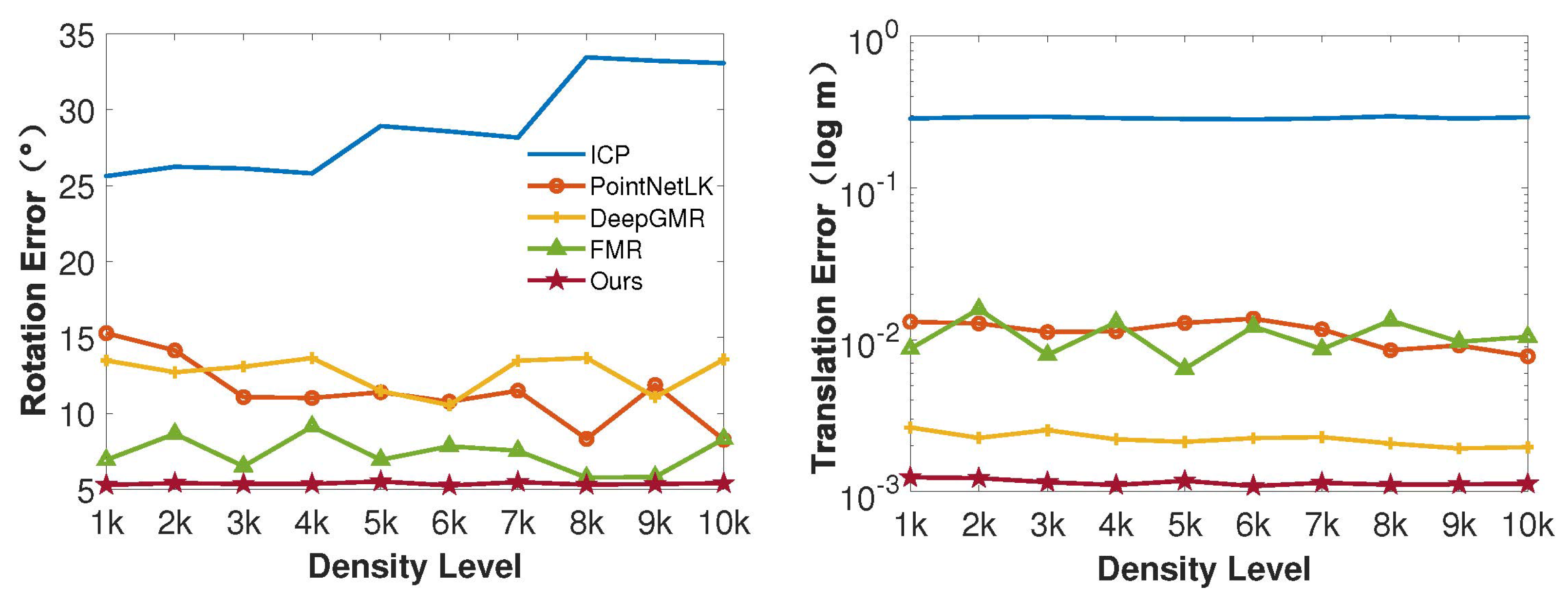
Comparison results of different density levels on the 7Scene dataset. The point numbers of the source and target point clouds range from 1 k to 10 k. In all registration experiments, our method maintains accuracy and robustness.
Figure 9.
Comparison results of different density levels on the 7Scene dataset. The point numbers of the source and target point clouds range from 1 k to 10 k. In all registration experiments, our method maintains accuracy and robustness.
Figure 10.
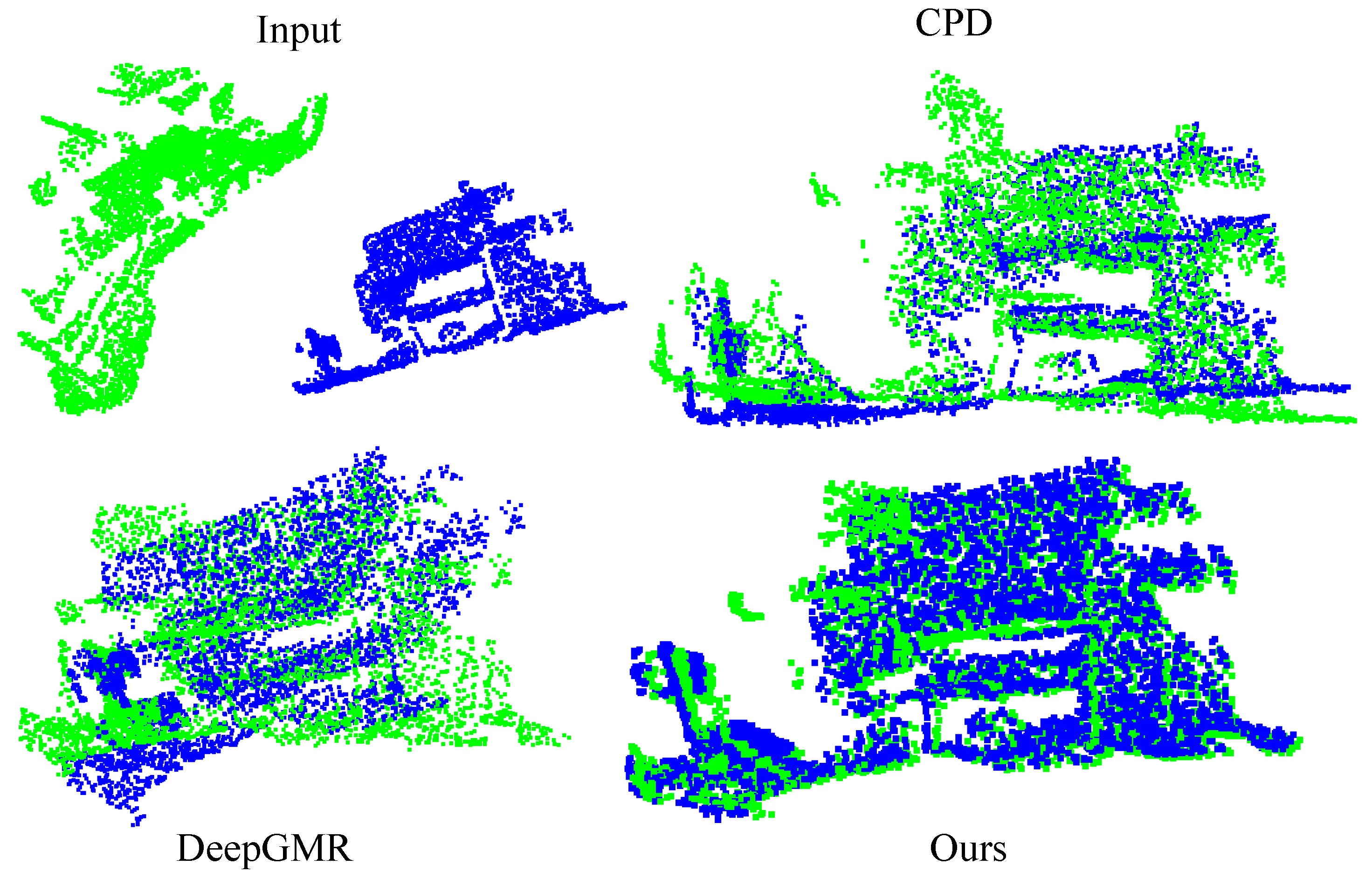
Qualitative registration results on partial data in the 7Scene dataset. The figures show the registration results of CPD, DeepGMR, and ours.
Figure 10.
Qualitative registration results on partial data in the 7Scene dataset. The figures show the registration results of CPD, DeepGMR, and ours.
Table 1.
ModelNet40: Comparison results of the unseen categories without Gaussian noise. The best results are displayed in bold, while the second-best results are underlined.
Table 1.
ModelNet40: Comparison results of the unseen categories without Gaussian noise. The best results are displayed in bold, while the second-best results are underlined.
| | Rotation Error () | Translation Error (m) |
|---|
| | RMSE ↓ | MAE ↓ | RMSE ↓ | MAE ↓ |
|---|
| ICP | 30.351408 | 23.879347 | 0.291203 | 0.250332 |
| FGR | 25.922915 | 22.460184 | 0.006555 | 0.004499 |
| CPD | 4.786544 | 0.762930 | 0.003145 | 0.000309 |
| PointNetLK | 9.047126 | 1.736442 | 0.039545 | 0.006354 |
| DeepGMR | 4.902193 | 2.541245 | 0.003074 | 0.002126 |
| DCP | 2.682713 | 1.802736 | 0.005024 | 0.003697 |
| FMR | 5.939945 | 1.234902 | 0.020327 | 0.003700 |
| Ours | 3.064052 | 1.609843 | 0.001325 | 0.000938 |
Table 2.
ModelNet40: Comparison results of the test on ModelNet40. The point numbers of two point clouds are both 512. The best results are displayed in bold, while the second-best results are underlined.
Table 2.
ModelNet40: Comparison results of the test on ModelNet40. The point numbers of two point clouds are both 512. The best results are displayed in bold, while the second-best results are underlined.
| | Rotation Error () | Translation Error (m) |
|---|
| | RMSE ↓ | MAE ↓ | RMSE ↓ | MAE ↓ |
|---|
| ICP | 39.799759 | 36.863148 | 0.288150 | 0.250225 |
| FGR | 16.473726 | 5.050144 | 0.040978 | 0.015393 |
| CPD | 9.001674 | 4.457861 | 0.003620 | 0.028238 |
| PointNetLK | 19.243651 | 4.851967 | 0.029123 | 0.005638 |
| DeepGMR | 4.770106 | 2.563812 | 0.003002 | 0.002057 |
| DCP | 38.305710 | 21.316710 | 0.009296 | 0.006652 |
| FMR | 10.119906 | 3.569691 | 0.019505 | 0.007553 |
| Ours | 3.373327 | 1.880049 | 0.001526 | 0.001117 |
Table 3.
ModelNet40: Comparison results of the test on the expanded transformation. The best results are displayed in bold, while the second-best results are underlined.
Table 3.
ModelNet40: Comparison results of the test on the expanded transformation. The best results are displayed in bold, while the second-best results are underlined.
| | Rotation Error () | Translation Error (m) |
|---|
| | RMSE ↓ | MAE ↓ | RMSE ↓ | MAE ↓ |
|---|
| ICP | 48.183731 | 44.349880 | 0.288150 | 0.250225 |
| FGR | 26.298521 | 10.552604 | 0.051524 | 0.022009 |
| CPD | 19.917654 | 9.409087 | 0.041613 | 0.030905 |
| PointNetLK | 38.747494 | 16.434245 | 0.047938 | 0.016704 |
| DeepGMR | 9.328154 | 4.062377 | 0.003980 | 0.002622 |
| DCP | 11.718525 | 5.886914 | 0.003053 | 0.002211 |
| FMR | 26.887462 | 12.422495 | 0.039190 | 0.018913 |
| Ours | 6.220909 | 3.203493 | 0.001616 | 0.001138 |
Table 4.
ModelNet40: Comparison results of the test on partial data. The point numbers of two point clouds are 1024 and 921, respectively.
Table 4.
ModelNet40: Comparison results of the test on partial data. The point numbers of two point clouds are 1024 and 921, respectively.
| | Rotation Error () | Translation Error (m) |
|---|
| | RMSE ↓ | MAE ↓ | RMSE ↓ | MAE ↓ |
|---|
| ICP | 25.922915 | 22.460186 | 0.494428 | 0.410775 |
| FGR | 27.229246 | 10.612548 | 0.053987 | 0.027252 |
| CPD | 11.553748 | 5.624317 | 0.042879 | 0.032712 |
| PointNetLK | 28.036747 | 11.787026 | 0.066898 | 0.040418 |
| DeepGMR | 24.422211 | 11.974214 | 0.041303 | 0.036290 |
| DCP | 31.406713 | 18.313848 | 0.044668 | 0.038792 |
| FMR | 28.328537 | 14.110557 | 0.045046 | 0.029118 |
| Ours | 8.340002 | 4.352821 | 0.043925 | 0.038332 |
Table 5.
7Scene: Comparison results of the test on real-world scenes. The best results are displayed in bold, while the second-best results are underlined.
Table 5.
7Scene: Comparison results of the test on real-world scenes. The best results are displayed in bold, while the second-best results are underlined.
| | Rotation Error () | Translation Error (m) |
|---|
| | RMSE ↓ | MAE ↓ | RMSE ↓ | MAE ↓ |
|---|
| ICP | 25.621710 | 22.087355 | 0.285877 | 0.246103 |
| FGR | 32.466103 | 17.400328 | 0.026984 | 0.012873 |
| CPD | 13.185246 | 7.772848 | 0.037270 | 0.028007 |
| PointNetLK | 15.288235 | 2.812165 | 0.013135 | 0.002467 |
| DeepGMR | 13.488777 | 6.892267 | 0.002648 | 0.001648 |
| DCP | 5.859264 | 3.314787 | 0.005533 | 0.003899 |
| FMR | 6.939286 | 1.400840 | 0.008716 | 0.001800 |
| Ours | 5.295327 | 3.909664 | 0.001243 | 0.000864 |
Table 6.
7Scene: Comparison results of the test on partial real-world scenes.
Table 6.
7Scene: Comparison results of the test on partial real-world scenes.
| | Rotation Error () | Translation Error (m) |
|---|
| | RMSE ↓ | MAE ↓ | RMSE ↓ | MAE ↓ |
|---|
| ICP | 25.922913 | 22.460184 | 0.356067 | 0.292270 |
| FGR | 16.824322 | 9.779890 | 0.033003 | 0.021518 |
| CPD | 17.643698 | 10.207256 | 0.047480 | 0.034908 |
| PointNetLK | 13.717697 | 6.552353 | 0.034506 | 0.021542 |
| DeepGMR | 28.637363 | 17.125318 | 0.025591 | 0.021899 |
| DCP | 9.964090 | 7.042327 | 0.026280 | 0.022408 |
| FMR | 43.034859 | 30.941980 | 0.054910 | 0.039119 |
| Ours | 7.464927 | 5.561217 | 0.025730 | 0.021929 |
Table 7.
Comparison results of the ablation study on the noisy ModelNet40 dataset ().
Table 7.
Comparison results of the ablation study on the noisy ModelNet40 dataset ().
| | Rotation Error () | Translation Error (m) |
|---|
| | RMSE ↓ | MAE ↓ | RMSE ↓ | MAE ↓ |
|---|
| DeepGMR | 6.416541 | 2.774974 | 0.003053 | 0.002131 |
| Ours-V1 | 3.146087 | 1.535921 | 0.003167 | 0.002299 |
| Ours-V2 | 3.103110 | 1.627020 | 0.001301 | 0.000921 |
Table 8.
Comparison of registration runtime results for different algorithms.
Table 8.
Comparison of registration runtime results for different algorithms.
| | Registration Runtime (ms) |
|---|
| | ModelNet40 | 7Scene |
|---|
| | 1024 | 1 k | 5 k | 10 k |
|---|
| ICP | 1.16 | 486.48 | 506.50 | 535.04 |
| FGR | 26.80 | 507.22 | 587.40 | 896.00 |
| CPD | 6.36 | 490.74 | 493.65 | 509.09 |
| PointNetLK | 64.32 | 156.96 | 261.15 | 454.83 |
| DeepGMR | 3.72 | 485.04 | 480.81 | 494.96 |
| DCP | 11.95 | 493.92 | 1828.99 | 2431.65 |
| FMR | 22.23 | 479.49 | 479.18 | 478.65 |
| Ours | 9.20 | 486.61 | 535.36 | 646.58 |
