Article

Spatiotemporal Change in Evapotranspiration across the Indus River Basin Detected by Combining GRACE/GRACE-FO and Swarm Observations

1
School of Architecture and Civil Engineering, Chengdu University, Chengdu 610106, China
2
Key Laboratory of Earthquake Geodesy, Institute of Seismology, China Earthquake Administration, Wuhan 430071, China
3
Gravitation and Earth Tide, National Observation and Research Station, Wuhan 430071, China
4
College of Natural Resources and Environment, South China Agricultural University, Guangzhou 510642, China
5
Department of Surveying Engineering, School of Civil and Transportation, Guangdong University of Technology, Guangzhou 510642, China
*
Author to whom correspondence should be addressed.
These authors contributed equally to this work.
Remote Sens. 2023, 15(18), 4469; https://doi.org/10.3390/rs15184469
Submission received: 25 July 2023 / Revised: 5 September 2023 / Accepted: 6 September 2023 / Published: 11 September 2023
(This article belongs to the Special Issue GRACE for Earth System Mass Change: Monitoring and Measurement)

Abstract

:
Evapotranspiration (ET) is an important approach for enabling water and energy exchange between the atmosphere and the land, and it has a very close relationship with terrestrial water resources and the ecological environment. Therefore, it is of great scientific to accurately quantify the spatiotemporal change in ET and its impact factors to understand the terrestrial water change pattern, maintaining water resource security and protecting the ecological environment. Our goal is to study the spatiotemporal characteristics of ET in the Indus River basin (IRB) and their driving factors. In our study, we first integrated the multi-source satellite gravimetry observations using the generalized three-cornered hat and least square methods to obtain the high-precision and continuous spatiotemporal evolution features of ET in the IRB from 2003 to 2021. Finally, we combined nine hydrometeorological and land cover type data to analyze the factors influencing ET. The results indicate that the algorithm used in our study can improve the ET accuracy by 40%. During the study period, ET shows a significant increasing trend (0.64 ± 0.73 mm/a), and the increasing rate presents spatial distribution characteristics of high variability in the northern areas and low variability in the southern areas of the study region. ET has a close relationship with precipitation, specific humidity, total canopy water storage, surface temperature and wind speed (with a correlation coefficients greater than 0.53 and variable importance of projection greater than 0.84). Among these factors, precipitation, specific humidity and surface temperature have significant correlations with ET (correlation coefficients greater than 0.85 and variable importance of projection greater than 1.42). And wind speed has a more significant positive effect on ET in the densely vegetated regions. The impacts of climate change on ET are significantly greater than those of land cover types, especially for similar land cover types. Ice and snow are significantly different to other land cover types. In this region, ET is only significantly correlated with precipitation, specific humidity and snow water equivalent (variable importance of projection greater than 0.81), and the impacts of precipitation and specific humidity on ET have been significantly weakened, while that of snow water equivalent is significantly enhanced. Our results contribute to furthering the understanding of the terrestrial water cycle in subtropical regions.

1. Introduction

Global warming and human activities have massive impacts on the terrestrial water cycle and have changed the natural hydrological system, resulting in a significant increase in the frequency of extreme heat, flood and drought events [1,2,3]. Due to these extreme disasters, affected ecosystems are significantly diminished [4,5]. Evapotranspiration (ET) is closely related to the water, energy and carbon cycle, reflecting the interactions between terrestrial, atmosphere and ocean environments [6,7]. The ET anomaly caused by natural and human factors alter the distribution of water vapor and turbulent energy flux, and they also affect temperature, atmospheric circulation, precipitation (PPT) and runoff and have an important impact on regional water resource changes and their spatiotemporal distribution [8,9]. Therefore, it is of great scientific value and social significance to accurately estimate ET change to master regional water resources, ensuring water resource security, evaluating the sustainability of ecosystems, and understanding the interaction between land and atmosphere [10,11].
The Indus River is an important water source used for agricultural irrigation in Pakistan, and the Pakistani economy is dominated by agriculture, with agricultural output accounting for 22% of GDP [12]. A previous study showed that extreme climatic events have shown to be significant factors in the major decline of water resources noted in recent years [13]. Due to the close relationship between ET and extreme climatic events, it is great socio-economic value to discuss the spatiotemporal evolution characteristics of ET in the Indus River basin (IRB) to maintain regional water security, ensure social stability and promote economic development. Previous studies of ET in the IRB have mainly relied on ground stations and remote sensing technology [14,15]. Although some studies’ results have been obtained, there are also certain limitations. Due to the low socio-economic development level, the ground stations are present in insufficient numbers and have an uneven distribution, meaning that they cannot meet the requirements for full coverage of the IRB. Although remote sensing technology can achieve full coverage, it cannot directly obtain the required hydrometeorological observations, which poses a huge issue regarding the uncertainty of study results [16]. Therefore, there is an urgent need to acquire novel data or a method to monitor ET in the IRB.
The successful application of gravity recovery and climate experiment (GRACE) and its follow-on (GRACE-FO) missions enable the comprehensive understanding of the terrestrial hydrology. GRACE/GRACE-FO satellites not only have the characteristics of all-weather and full coverage, but can also directly observe the time variable signals of terrestrial water with high precision [17,18]. Since Rodell first proposed the ET estimation method based on GRACE/GRACE-FO observations, GRACE/GRACE-FO data have been continuously used in regional ET studies, such as in the Yellow River basin [19], the Three Gorges Reservoir [20], the United States [21] and the Lake Chad basin [22]. However, the above studies did not take into account the discontinuity of observations caused by an 11-month data gap between GRACE/GRACE-FO missions. This discontinuity has brought certain difficulties to the research work [23,24]. The emergence of the Swarm mission has brought hope of solving the above problems, and its task period only covers the above gap and has the ability to detect the Earth’s time variable gravity signals [25,26,27]. Many scientists have applied Swarm observations to the study of droughts and ice sheet mass change [28,29,30]. However, to the best of our knowledge, there is no literature on ET detection in the IRB based on either GRACE/GRACE-FO observation or combining GRACE/GRACE-FO and Swarm observations to detect global or regional ET. In addition, due to the different mathematical models and methods used by different institutions when calculating GRACE/GRACE-FO data, there are certain discrepancies in the terrestrial water storage change (TWSC) estimated via different GRACE/GRACE-FO solutions. The discrepancy creates considerable uncertainty in the study results. This issue is not considered in previous studies of regional ET.
The main objectives of our work are as follows: (1) to evaluate the uncertainty of TWSC results estimated via different GRACE/GRACE-FO solutions using the generalized three-cornered hat (GTCH) method; (2) to reduce the uncertainty of TWSC results based on the fusion method; (3) to detect the spatiotemporal change in ET in the IRB by combining GRACE/GRACE-FO and Swarm solutions; (4) to analyze the impacts of hydrometeorological factors and land cover type on ET in the IRB. In our paper, the study area, data and method were introduced in Section 2 and Section 3, respectively. The results and analysis were shown in Section 4. The discussion and summary are shown in Section 5 and Section 6, respectively.

2. Study Area

The IRB is located in South Asia, and its geographical range is 24–37°N and 66–82°E (Figure 1). The Indus River originates from the Qinghai–Tibet Plateau, flows between the Himalayas and Karakoram Mountains, flows in a southwestern direction and runs through the Himalayas; the right bank meets the Kabul River, and the left bank meets the Punjab Tributaries, and it flows through Pakistan to the Arabian Sea. The IRB belongs to the subtropical climate zone with obvious monsoon climate characteristics, but due to the barrier of the mountains in the northeastern area, the climate ranges between semi-arid and arid and tropical and subtropical in nature. The highest and lowest temperatures in the basin are about 46 °C and −15 °C, and the average PPT is about 300 mm per year. The annual runoff of the Indus River is about 144 billion m3. Except for the mountainous parts of Pakistan, the IRB is the driest part of the subcontinent. The level of social and economic development in this region is low, and the national economy is mainly based on agriculture, which is highly dependent on water resources. Therefore, our results can help local governments to formulate reasonable water resource allocation policies and ensure the sustainable development of local social economies.

3. Data

3.1. GRACE/GRACE-FO Data

To obtain monthly TWSC gridded data between 2003 and 2021 at a spatial resolution 1° × 1°, we used the three GRACE/GRACE-FO RL06 spherical harmonic (SH) solutions. Before the TWSC data were estimated, these SH solutions experienced a series of pre-processing alterations, including coefficient substitution, filtering, scale recovery, etc. [31], which were provided by the Center for Space Research at the University of Texas at Austin (CSR), the Helmholtz-Centre Potsdam-German Research Centre for Geosciences (GFZ) and the Jet Propulsion Laboratory (JPL). For convenience, GRACE and GRACE-FO are called GRACE for short, and three SH solutions were called CSR-SH, GFZ-SH and JPL-SH, respectively.

3.2. Swarm Data

In our study, the Swarm SH solution from 2014 to 2021 was derived from the International Combination Service for Time-Variable Gravity. This service is a combination of Swarm solutions derived from four institutions (the Institute of Geodesy at the Graz University of Technology, the Astronomical Institute at the Czech Academy of Sciences, the University of Bern and Ohio State University) based on a variance component estimation method [32]. The Swarm SH solution also needs to be pre-processed before the calculation of TWSC gridded data. In addition to the different filter parameters (1000 km Fan filter), the other pre-processing stages are the same as those of the GRACE SH solution.

3.3. PPT, ET and Runoff Data

The monthly 0.5° × 0.5° PPT, ET and runoff gridded data from 2003 to 2021 were provided by the Global Land Surface Reanalysis Products of the China Meteorological Administration (CMA-RA/Land). The CMA-RA/Land was estimated using the set multi-source fusion method, assimilation algorithm, surface parameter optimization approach and Noah 3.3 land surface model.

3.4. Other ET Products

3.4.1. GLDAS Products

The Global Land Data Assimilation System (GLDAS) 2.1 model was sourced from the Goddard Space Flight Center at the National Aeronautics and Space Administration and the National Centers for Environmental Prediction at the National Oceanic and Atmospheric Administration, and it is based on different land surface hydrological models. The driving data of this model were determined by combing the measured data of land sites and remote sensing observations. The global terrestrial ET results were estimated and simulated according to hydrological simulation and data assimilation technology [33].

3.4.2. GLEAM Products

The Global Land Evaporation Amsterdam Model (GLEAM) 3.6a was jointly developed and provided by Regent University in Belgium and Vrije Universiteit Amsterdam in the Netherlands [34,35], and it provided the monthly ET gridded data at a spatial resolution 0.25° × 0.25°. The ET data were calculated using multi-source remote sensing and reanalysis PPT data based on the Priestley–Tylor formula [36].

3.4.3. A Harmonized Global Land Evaporation Dataset from Model-Based Products Covering the Period 1980–2017 (AHGLED)

The dataset with a spatial resolution 0.25° × 0.25° was based on the three widely used model-based ET datasets, namely ERA5, MERRA2 and GLDAS 2.1 Noah reanalysis data. The variation coefficient was used to select the fusion region with high concordance, and the dataset was obtained by fusing the above three ET data based on the reliable ensemble averaging method. The results show that the AHGLED ET data capture ET trends in different regions well and perform well under all vegetation cover scenarios [37].

3.5. Other Hydrometeorological Data

In our study, the hydrometeorological data include surface temperature (ST), soil moisture (SM), specific humidity (SH), total canopy water storage (TCWS), wind speed (WS), groundwater (GW) and snow water equivalent (SWE). Among these factors, monthly ST, SM, SH, TCWS, WS and SWE gridded data came from the CMA-RA/Land between 2003 and 2020, the spatial resolution of which was 0.5° × 0.5°, and the GLDAS 2.1 model provided the monthly 0.25° × 0.25° GW gridded data.

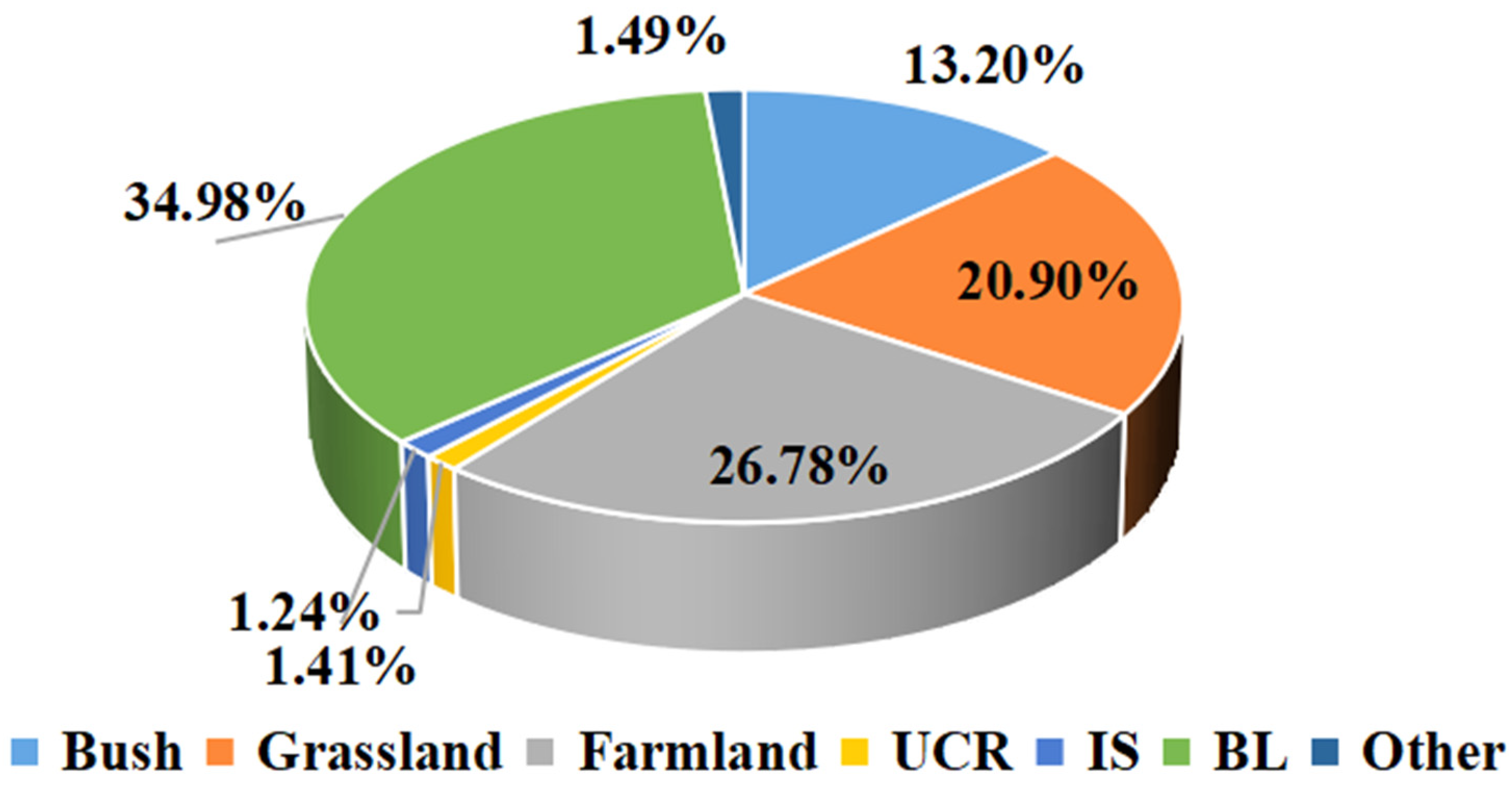
3.6. Land Cover Type Data

The land cover type gridded data were provided by the MODIS land vegetation cover classification product’s sixth edition. The product with a spatial solution of 500 × 500 m was estimated via the observations obtained from Terra and Aqua, which contain the main land cover types in the world at present [38,39]. Figure 2 shows the proportion of area occupied by each land cover type in the IRB.

4. Methods

In our study, we first assessed the uncertainty of the three TWSC results derived from different GRACE solutions using GTCH approach. Then, according to the uncertainty results, three TWSC results were fused based on the least square approach to reduce the uncertainty of TWSC result. Subsequently, we combined fused TWSC and Swarm TWSC to construct a 19-year ET continuous time series in the IRB. Finally, we estimated the impact of nine hydrometeorological factors and land cover types on ET in the IRB.

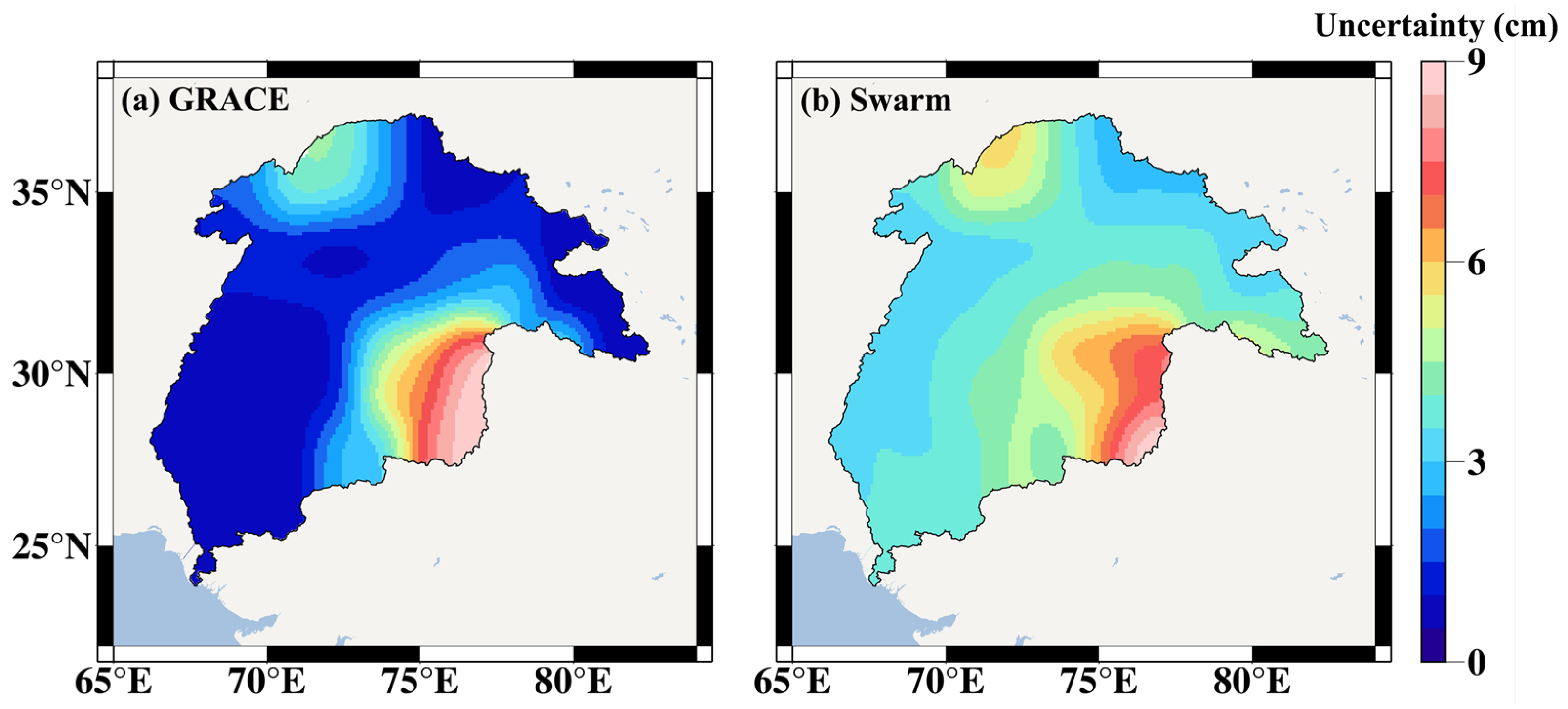
4.1. Uncertainty of TWSC

The uncertainty of the experimental data has a very important impact on the experimental results. Due to different mathematical models and methods, there are certain discrepancies in the TWSC results estimated via GRACE solutions provided by different institutions. These discrepancies introduced uncertainty to our results [40]. To reduce the uncertainty of our results, we used the GTCH and least square approaches to process three GRACE TWSCs. Compared to other methods, the GTCH approach could realize the evaluation of data uncertainty without prior information [10,41]. The specific technical details of this method can be seen in Ref. [42].
According to the relative covariance of different datasets derived via the GTCH method, we fused the different datasets by taking their weighted average.
X = i = 1 N k i X i i = 1 , 2 , , N
where  X i  and  p i  are the TWSC results derived via the individual GRACE solutions and its corresponding weight, respectively. The weights were determined based on the estimated variances.
k i = 1 / r i i n = 1 N 1 / r n n
where  r i i i = 1 , 2 , , 6  is the variance of the ith TWSC time series estimates determined via the GTCH method. The above process was performed grid by grid until we fused the TWSC results from the six GRACE solutions on all of the grid nodes.

4.2. ET Estimation

Based on the water balance equation, the expression of ET in the basin is as follows [43]:
E T = P R d s d t
where  P  and  R  represent PPT and runoff data in the basin, respectively.  d s / d t  represents the terrestrial water storage change.
d s d t = T W S A t + 1 T W S A t 1 2 Δ t
where  Δ t  represents the temporal resolution of TWSC result;  T W S A t 1  and  T W S A t + 1  represent the terrestrial water storage anomalies in the  t + 1  and  t 1  months, respectively.
Before GRACE appeared, it was very difficult to estimate the terrestrial water storage anomalies. Therefore, the terrestrial water storage anomalies were often ignored when estimating ET in the basin. The expression is
E T = P R

4.3. Evaluation Indicators

In this study, we used the other ET products to evaluate our result based on the three indicators, including correlation coefficient I, root mean square error (RMSE), Nash–Sutcliffe efficiency (NSE) and Lin’s concordance correlation coefficient (LCCC). The expressions of these indicators are as follows [26,44,45,46]:
r = i = 1 N x i x ¯ y i y ¯ i = 1 N x i x ¯ 2 i = 1 N y i y ¯ 2 i = 1 , 2 , , N
R M S E = i = 1 N x i y i 2 N
N S E = 1 i = 1 N x i y i 2 i = 1 N x i x ¯ 2
L C C C = 2 σ x y σ x 2 + σ y 2 + x ¯ y ¯ 2
where  x  represents the GRACE ET series;  y  represents the ETs derived via other approaches;  x i  and  y i  represent the  i th value in the  x  and  y  time series, respectively;  x ¯  and  y ¯  represent the average values of  x  and  y , respectively;  σ x  and  σ y  represent the variance of  x  and  y , respectively;  σ x y  represents the covariance of  x  and  y ; and  N  represents the number of observations  x  and  y .

4.4. Partial Least Squares Regression Model

The partial least squares regression model (PLSR) can estimate the relationship between multiple independent and dependent variables. Its advantage lies in fully considering the correlation between different independent variables. In our study, we applied the PLSR method to evaluate the impacts of various hydrometeorological elements on ET. ET is the dependent variable, and different independent variables are the independent variables. The variable importance of projection (VIP) can accurately estimate the influence level of hydrometeorological factors on regional ET. The specific expression of VIP is as follows [47]:
V I P j = n i = 1 m R d Y , v i w i j 2 i = 1 m R d Y , v i j = 1 , 2 , , n
where  n  is the number of hydrometeorological factors, and  V I P j  is the VIP value of the  j th hydrometeorological factor.  v i i = 1 , 2 , , m  represents the  m  principal components of  Y Y  represents FPI, and  w i j  represents the weight of each element in the matrix after the matrix  X  is standardized.  X  represents a matrix composed of the observations of  n  hydrometeorological factors, and  R d Y , v i = r 2 Y , v i  and  r Y , v i  represent the correlation coefficients between  Y  and  v i , respectively. And a VIP larger than 0.8 means that the factor has a significant impact on ET [48].

5. Results

5.1. Construction of Combined TWSC Observations

To reduce the impact of the uncertainty of GRACE TWSC, we performed fusion processing on the three GRACE TWSCs. Figure 3 shows that the fused TWSC results are consistent with the three GRACE TWSC results, having the same peaks, troughs and change trends. And the fused TWSC result has a strong correlation with three GRACE TWSC results (all correlation coefficients are greater than 0.86). And the fused TWSC result has a smaller uncertainty level (1.11 cm) than those of the three GRACE TWSC results (CSR-SH, 1.32 cm; GFZ-SH, 1.33 cm; JPL-SH, 1.86 cm). The above results explain that the fused TWSC result not only retains the reliability of the original TWSC result, but also effectively reduces the uncertainty level of the TWSC result. Therefore, we used the fused TWSC result as the GRACE result in the follow-up study.
In Figure 3, the TWSC time series has a disruption (from July 2017 to May 2018) due to the lack of a tight interface between GRACE and GRACE-FO missions. The GRACE satellites stopped working in July 2017, while the GRACE-FO satellites were launched in April 2018 and started working in the next month. To fill this gap, we used the Swarm TWSC result in our study. As the Swarm mission period extends from January 2014, we compared the GRACE and Swarm TWSC results derived during 2014 and 2021. Figure 4 and Table 1 show that Swarm TWSC has similar peaks, troughs and change trends to those of GRACE TWSC. However, the fluctuation range of Swarm TWSC is significantly greater than that of GRACE due to the greater uncertainty of Swarm TWSC [23]. Figure 5 shows that the uncertainties of GRACE and Swarm TWSC have the same spatial distribution. In most regions, the uncertainties of GRACE TWSC are lower than 2 cm, while those of the Swarm TWSC are mainly concentrated between 3 and 6 cm.
In Figure 6, we used GRACE and Swarm TWSC to construct 19 consecutive years of TWSC time series (GRACE/Swarm TWSC) in the IRB, using data derived between 2003 and 2021. To evaluate the reliability of the combined TWSC result, we compared the GRACE/Swarm and GLDAS TWSC. The results show that the two TWSC results have the similar peaks, troughs and change trends. However, GLDAS TWSC result (−0.12 ± 0.61 mm/a) shows a smaller decreasing rate than that of GRACE/Swarm (−4.32 ± 0.41 mm/a). This result occurs because the GLDAS TWSC result only reflects the naturally induced TWSC, while the GRACE/Swarm result is the sum of the naturally and human-induced TWSC. Previous studies [49,50] show declining TWSC in the IRB due to the high water withdrawals required for agricultural irrigation.

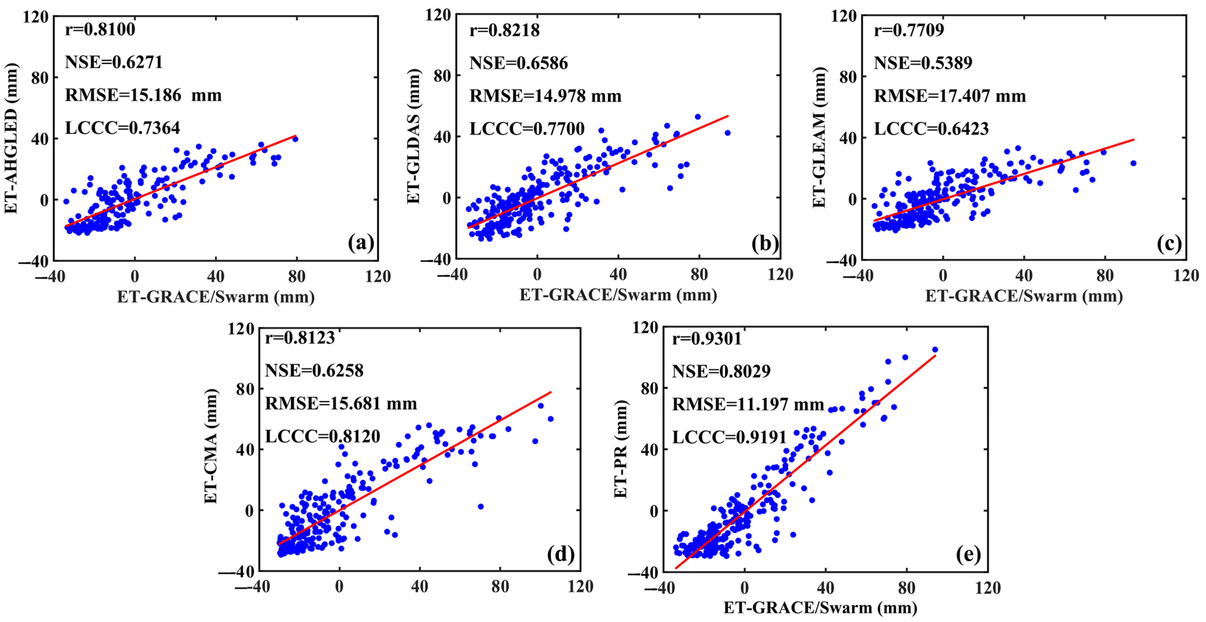
5.2. Evaluation of ET Result Based on GRACE and Swarm Results

In our study, the GRACE/Swarm TWSC result was used to estimate ET (ET-GRACE/Swarm) in the IRB between 2003 and 2021. In Figure 7 and Figure 8, we used five ET results from the GLDAS (ET-GLDAS), GLEAM (ET-GLEAM), CMA-RA/Land (ET-CMA), AHGLED (ET-AHGLED) and water balance methods based on PPT and runoff data (ET-PR) to examine the quality of ET-GRACE/Swarm (Figure 7 and Figure 8). In Figure 7, six time series of ET results show significant periodicity, and they have the same peaks and troughs. All ET results are mainly concentrated between −30 mm and 100 mm. The time series of ET-GRACE and ET-PR are the closest, and the amplitude of their results are significantly larger than those of the other ET results. This result occurs because they include nature- and human-induced ET, while other ET results only consider the nature-induced ET.
We calculated the correlation coefficient(r), NSEs, RMSEs and LCCCs between ET-GRACE/Swarm and the other five ET results to precisely quantify their discrepancy (Figure 8). Since the time span of ET-AHGLED is only 2003 to 2017, all ET data were limited to the period 2003–2017. The correlation coefficient, NSE and LCCC between ET-GRACE and ET-PR are the greaterst, which are 0.9301, 0.8029 and 0.9191. respectively. And their RMSE is very small (11.197 mm), which shows that they have a very high consistency. Combining the correlation coefficient, NSE and RMSE and LCCC, we ranked the five ET results according to their degree of agreement with ET-GRACE. The order is ET-PR, ET-CMA, ET-GLDAS, ET-AHGLED and ET-GLEAM. In general, ET-GRACE has a strong correlation with the other five ET results (r > 0.77), their NSEs and LCCCs are greater than 0.5 and 0.64, respectively, and their RMSEs are smaller than 17 mm. This result indicates that the performance of ET-GRACE in the IRB agreed well with the other five ET products.

5.3. Spatiotemporal Distribution of ET in the IRB

ET-GRACE/Swarm exhibits a significant seasonal variation characteristic (Figure 9). The red regions (high ET) are mainly concentrated in summer, while the blue regions (low ET) are mainly concentrated in autumn. This result means that the peak and trough of ET appear in summer and autumn. The maximum ETs (100 mm) appeared in summer of 2020, and the minimum ETs (−40 mm) occurred in autumn of 2012 and 2014. Figure 10a shows that the annual average ET in the IRB is 0.5 mm, and the variation range is −0.2~1.2 mm. The spatial distribution shows a gradually decreasing distribution trend in a northwest–southwest direction. Long-term trend changes in ET (Figure 10b) show increasing trends (0.7 mm/a) across most of the IRB, but there is a downward trend in parts of the northeastern area. The largest increasing rate (1.5–2.0 mm/a) occurs in the north–central region.

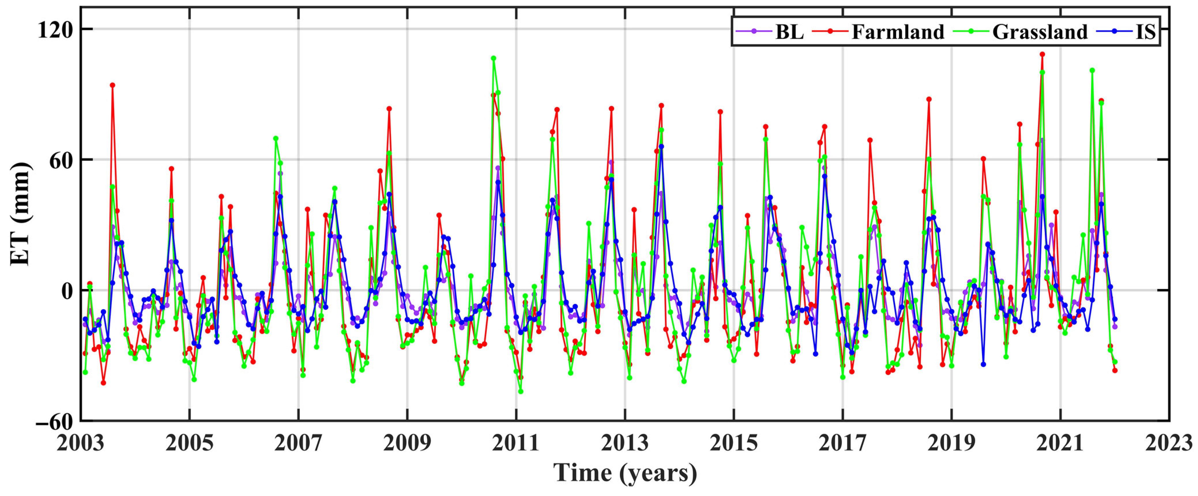
5.4. ET in the Different Land Cover Types

Figure 2 shows that the land cover types in the IRB are mainly BL (34.98%), farmland (26.78%), grassland (20.90%) and IS (13.20%), and the remaining land cover types accounted for only 4.14% of total land. Therefore, we focused on the discrepancy in ET in the four land cover types (BL, farmland, grassland and IS). The four ET time series (Figure 11) have the same peaks and troughs. Among these types, ETs in farmland and grassland have the larger fluctuations (−50~115 mm), while ETs in BL and IS have the smaller fluctuations (−30~65 mm). In Table 2, ET shows an increasing trend (0.80 ± 0.62 mm/a) in the IRB. Except for IS, the long-term change trends of ETs in the other three land cover types are increasing. This finding shows that BL, farmland and grassland have contributed to ET growth. Among these factors, the contribution of grassland is the greatest. ET in farmland has the largest annual amplitude (2.98 cm); the second highest figure is found in grassland (2.89 cm), and ET in the above two land cover types have larger annual amplitude than the one (2.36 cm) in the IRB. The smallest annual amplitude appears in the BL (1.41 cm). In summary, grassland and farmland are the most beneficial to ET among the four land cover types.
To further discuss the discrepancy between ETs in the different land cover types, we show the performance of ETs on three time scales (Figure 12). In Figure 12a, the largest annual ET appears in the IS (0.81 mm), followed by grassland (0.78 mm), farmland (0.71 mm) and BL (0.62 mm) regions. This result is not consistent with the area percentage of the four land cover types. It shows that the size of ET is independent of the area of the land cover type. Figure 12b shows the seasonal distributions of ET in the four land cover types. Except for IS, the ETs reach the maximum (farmland, 38.2 mm; grassland, 35.7 mm and BL, 12.4 mm) in summer, while the maximum ET (13.2 mm) in the IS appears in Autumn All the minimum ETs occur in winter. In summer, all the ETs are positive, and only the ET in the IS and BL are postive in autumn. Positive ET concentrates in summer, which is due to the greatest PPT occurring in this season. In Figure 12c, the largest ETs appear in July (farmland and grassland regions) and August (BL and IS regions), respectively, while the smallest ETs occur in December (farmland and grassland regions), July (BL region) and February (IS region). From the absolute value of ET changes, the fluctuations in grassland and farmland regions are the largest. Overall, the farmland and grassland regions have the largest ET changes, and the IS region has a different temporal distribution of ET with other three land cover types.

5.5. Impacts of Climate Change on ET in the IRB

The spatiotemporal evolution of ET is largely affected by climate change. To understand the relationship between climate change and ET, the two indicators (correlation coefficient and VIP) were used to evaluate the associations between the nine main hydrometeorological factors and ET (Table 3). In Table 3, SWE has a negative correlation with ET, while the other hydrometeorological factors have positive correlations in the IRB. And ET has a significant correlation with ST, TCWS, SH, PPT and WS in the IRB (correlation coefficient and VIP greater than 0.42 and 0.99, respectively). Among these factors, PPT and TCWS have very strong correlations with ET (correlation coefficient and VIP greater than 0.74 and 1.46, respectively). This result occurs because PPT and TCWS provide the required moisture to enable ET [51]. Vegetation transpiration is an important part of ET [52]. SH is also closely related to ET. With the intensification of ET, the content of water vapor in the air increases, which leads to the increase in SH [53]. ST represents energy, and the level of ST directly affects the intensity of ET activity. Goyal et al. [54] indicated that for every 8-degree increase in ST, ET increases by 14.8%. WS has a certain relationship with ET, but this relationship is relatively weak because the impact of WS on ET is indirect. Wind can increase air movement over the surface of the liquid, making it easier for moisture in the surface to evaporate [55].
To analyze the impacts of climate change on ET under different land cover types, we simultaneously precisely quantified the relationships between ET and nine hydrometeorological factors. Table 3 shows that the impacts of nine hydrometeorological factors on ET in the grassland and farmland regions are the same as that in the IRB. In the BL, the impacts of ST, TCWS, SH, PPT and WS on ET were weaken. Among, the impact of WS was most severely weaken (correlation coefficient ranged from 0.42 to 0.22). It may be related to the presence of less moisture in the BL. The impacts of other factors on ET are basically unchanged. In the IS, the result is a big change. PPT, ST, SH and SWE have a significant correlation with ET. Among, the relationship between SWE and ET was enhanced (correlation coefficient from −0.19 to −0.49; VIP from 0.15 to 1.40). It’s due to the greatly increased moisture provided by ice and snow to ET.
To discuss the impact of climate change on ET on the spatial scale, we plotted the spatial distributions of correlation coefficients and VIPs between ET and ST, TCWS, SH, PPT and WS in the IRB (Figure 13). In Figure 13, the correlation coefficient and VIP have a similar spatial distribution. This finding suggests that the results of two evaluation indicators are basically the same. Figure 13a,b show the spatial distribution of the correlation coefficient and VIP between ST and ET. The correlation between ST and ET has distinct spatial distribution characteristics, that is, high variability in the eastern areas and low variability in the western areas. The higher correlations are mainly concentrated in the upper reaches, where IS dominates (Figure 1b). Due to the rise in ST, the melting of ice and snow speeds up, which provide sufficient water for ET. Among these factors, the maximums appear in the northern area (correlation coefficient and VIP are 1.00 and 1.35), while the minimums occur in the western area (correlation coefficient and VIP close to 0). The correlations between TCWS and ET show significant north–south distribution characteristics, that is, the correlation in the northern area is low, and the correlation in the southern area is high (Figure 13c,d). The closer to area is to the southeastern region, the higher the correlation because the region is dominated by bush, grassland and farmland (Figure 1b). The maximums appear in the delta region (correlation coefficient and VIP are 1.0 and 2.0, respectively) because the delta region is dominated by wetland and farmland. In Figure 13e,f, SH has a strong correlation with ET in most regions. Only in the northern area are the correlations relatively weak (correlation coefficients and VIPs close to 0). The correlations between SH and ET represent an east–west distribution feature, that is, the correlations in the eastern area are greater than those in the western area. This finding is related to the fact that the eastern region is mostly densely vegetated. Comparing Figure 13c–f, we found that the spatial distributions of the correlation of TCWS and SH are the most similar. This finding shows that the regions with dense vegetation are more conducive to ET. Figure 13g,h show that PPT and ET have a strong correlation in most regions (correlation coefficients and VIPs greater than 0.9 and 1.7, respectively). The maximums appear in the northwestern area (correlation coefficient and VIP are 1.0 and 3.5, respectively). The correlations between WS and ET show a significant north–south distribution feature, that is, the correlations in the southern area are stronger than those in the northern area (Figure 13i,j) because the southern regions are closer to the ocean and more prone to windy weather.
As there is a delay in the interactions between the hydrometeorological factors, we calculated the maximum correlation coefficients and delay months between ET and six hydrometeorological factors in the IRB and areas with different land cover types (Figure 14). In Figure 14a, ET has a strong correlation with ST, TCWS, SH, PPT and WS in the IRB (all correlation coefficients are greater than 0.57). Among these factors, the correlation coefficient between ST and ET is the smallest (0.57). The response times of ET to ST, TCWS, SH and PPT are 0 months, but the response time of ET to WS is 1 month. This finding is due to the indirect impact of WS on ET [55]. Comparing Figure 14a–d, the relationships between ET and ST, TCWS, SH, PPT and WS in the grassland, farmland and BL regions are the most similar to those in the IRB, that is, the correlation order of five hydrometeorological factors is the most consistent. Among three land cover types, the correlations between ET and ST, SH, PPT and WS are the largest in the farmland region, while that between ET and TCWS is the largest in the grassland region. This finding indicates that ET in the farmland region is more vulnerable to climate change, and vegetation transpiration activity in the grassland region is more active than that in the farmland region. Figure 14e shows that the impact of PPT on ET is weaken (correlation coefficient from 0.97 to 0.70), which is smaller than the one of SH. The response time of ET to SH and PPT increase (from 0 month to 1 month). And SWE has a significant correlation with ET (correlation coefficient is −0.52). This finding demonstrates that the proportion of moisture provided by SWE to ET is increasing, while that provided by PPT to ET is decreasing. However, the moisture provided by PPT is relatively large. In the IS, the process of ET is stretched, which may be due to the low temperature and dry environment.
To further understand the role played by ET in the land–atmosphere water cycle, we calculated the correlation coefficients and VIPs between nine hydrometeorological factors (Figure 15). TCWS has a stronger correlation with PPT than runoff and SMC, which shows that vegetation absorbs most of water brought by PPT. This result is consistent with the conclusion that TCWS is the terrestrial water component most strongly correlated with ET (Table 3). Comparing Table 3 and Figure 15, the correlations between runoff, SMC and PPT are the similar to that of ET. This result shows that the proportion of water distribution brought by PPT is consistent with that returned to the atmosphere by the terrestrial water. It preliminarily reveals the pattern of water exchange between the land and the atmosphere. ST has a strong correlation with WS because the two factors represent the reflection of energy.

6. Discussion

6.1. Influencing Factors of ET

In this study, we discussed the impacts of climate change and land cover type on ET in the IRB. The results show that except for IS, the impacts of climate change on ET in the other three land cover types are basically the same. A previous study [56,57] also indicated that the impacts of hydrometeorological factors on ET are much greater than that of the land cover type. We found that three similar land cover types (grassland, farmland and BL) have the same impacts of climate change on ET. IS has a great discrepancy compared to the three other land cover types, and the impacts of climate change on ET in the IS are significantly different to those of the three other land cover types. This result shows that the impacts of climate change on ET in the similar land cover types have few differences, but those in the land cover types with significant differences have great discrepancy. Therefore, the impacts of climate change on ET are negligible in the regions with similar land cover types in the follow-up study.
Different land cover types differently contribute to ET. Table 2 shows that the increasing rate of ET in the BL (0.35 ± 0.44 mm/a) is only half of that of farmland (0.68 ± 0.94 mm/a) and one-third of that of grassland (0.94 ± 0.77 mm/a). It demonstrates that relatively intense ET activity occurs in the regions with dense vegetation. Li et al. [58] showed that the ETs in the grassland and farmland are more severe that those in other land cover types. As vegetation transpiration is an important part of ET, the regions with denser vegetation have more intense vegetation transpiration. The ET changes in the farmland are less than those in the grassland, which may be attributed to the differences in the ETs of farmland at different agricultural production stages. Chen et al. [59] indicated that ET in farmland is significantly greater in the harvesting and planting stages than in the irrigation stage. In the IS, ET shows a decreasing trend (−0.11 ± 0.36 mm/a), which is significantly smaller than that in the other three land cover types due to the low temperature, less PPT, dry climate and short vegetation growth season [60].

6.2. Uncertainty of Observations

Different institutions have used different data processing strategies and background models, which can lead to some discrepancies between the phase, amplitude, period and location of the strongest signal in the TWSC signals [61,62]. Therefore, we may misinterpret the hydrological changes in the study region when only using a single model [63]. At present, the verification and evaluation of GRACE results mainly occur through comparisons with hydrological models [64,65], actual observations [66,67] and water balance methods [68,69]. However, these methods can be affected by hydrological model accuracy, hydrometric station coverage and human activities. The GTCH approach can evaluate the uncertainty of GRACE TWSC without knowing the real reference field. In our study, we used the GTCH approach to evaluate the uncertainty of three GRACE TWSC models. To reduce the uncertainty of GRACE TWSC models, we integrated the three GRACE TWSC using the least square approach according to the uncertainty results. The results show that our approach reduces the uncertainty of GRACE TWSC models from 1.86 cm to 1.11 cm, i.e., a 40% reduction in the uncertainty level. This approach significantly improves the reliability of our results.
In our study, we used Swarm TWSC to fill the data gaps between GRACE and GRACE-FO missions to ensure the continuity of observations. To maintain the reliability of our results, we also calculated the uncertainty of Swarm TWSC. By comparing GRACE to Swarm TWSC in the same period, we tested the reliability of Swarm TWSC for the IRB. Figure 4 and Figure 5 and Table 1 show that Swarm TWSC has good performance with GRACE TWSC in the IRB. Previous study [70] used GRACE and Swarm solutions to calculate the TWSC in the IRB and compared the trend change, average mass change, correlation coefficient, root mean square error and cycle repetition time of the two TWSC results. The results show that the Swarm solution has the better accuracy and can replace GRACE one to monitor TWSC in the IRB.

6.3. Limitation and Future Work

IRB is a region in which frequent human activities have changed the spatiotemporal distribution of ET. Unfortunately, our study did not provide a detailed analysis of the impact of human activities on ET in the IRB. Due to limited capacity, more accurate human activities data have not been collected. Therefore, in the follow-up study, we will investigate ways to separate human-induced ET from total ET and collect high-precision and high time-scale human activities data to discuss the impact of human activities on ET. And we will also use deep learning to extend the ET time series to explore the long-term change rule of ET and its causes.

7. Conclusions

Global warming and human activities have profoundly changed the spatiotemporal distribution features of global and regional ET. Therefore, it is of great significance to understand ET change patterns and their driving factors. Although many scholars have conducted a lot of studies of global and regional ET, there are certain limitations. To achieve the uninterrupted monitoring of regional ET with full coverage, all-weather abilities and high precision, we integrated GRACE/GRACE-FO and Swarm solutions to estimate ET in the IRB.
Firstly, we used the GTCH method to evaluate the uncertainties associated with the three GRACE TWSCs and fused three GRACE TWSCs to reduce the uncertainty of TWSC using the least square method. The results show that our approach improved the accuracy of the TWSC results by 40%.
Secondly, we applied the fused TWSC, PPT and runoff data to estimate ET in the IRB based on the water balance equation. To verify the reliability of our ET result, we used the correlation coefficient, RMSE, NSE and LCCC to measure the differences between our ET result and other ET data from five productions. The results indicate that our result has good performance with other five ET data in the IRB.
Finally, we discussed the relationships between ET and hydrometeorological factors, land cover types based on correlation coefficient and VIP. It was found that climate change has a more pronounced impact on ET than land cover type, and the impacts of climate change on ET are the same for the similar land cover types. The regions with dense vegetation have the greatest ET.
Our result helps to understand the basic process of Earth’s water cycle, and it is of great scientific value and social significance in terms of protecting the safety of water resources and preventing hydrological disasters.

Author Contributions

Conceptualization, L.C.; methodology, Z.Z. and L.C.; investigation, C.Y.; resources, C.X.; data curation, M.Y.; writing—original draft preparation, L.C.; writing—review and editing, C.Y. and L.C.; visualization, Y.M.; supervision, Y.L.; project administration, C.X.; funding acquisition, Z.Z. All authors have read and agreed to the published version of the manuscript.

Funding

This research was funded by the Open Fund of Wuhan, Gravitation and Solid Earth Tides, National Observation and Research Station (WHYWZ202102); the National Natural Science Foundation of China (41931074, 41974014, 42074172, 42004013, 42274004); the Science for Earthquake Resilience (XH21021); the Max Planck Society; and the Chinese Academy of Sciences within the LEGACY (“Low-Frequency Gravitational Wave Astronomy in Space”) collaboration (M.IF.A.QOP18098; Guangdong Basic and Applied Basic Research Foundation (2022A1515010469).

Data Availability Statement

GRACE RL06 data were derived from CSR, GFZ and JPL and the Swarm solution via COST-G: http://icgem.gfz-potsdam.de/series (accessed on 6 July 2023); PPT, runoff, WS, TCWS, SWE, SMC and ST gridded data were acquired via the following webpage: http://data.cma.cn (accessed on 6 July 2023); ET gridded data were acquired via the following link: sftp://hydras.ugent.be (accessed on 6 July 2023); GW gridded data derived from the GLDAS model were acquired via the following link: https://disc.gsfc.nasa.gov/datasets (accessed on 6 July 2023).

Acknowledgments

We are grateful to COST-G for providing Swarm solution; CSR, GFZ and JPL for providing GRACE solution; the China National Meteorological Science Data Center for providing PPT, ET, runoff, WS, TCWS, SWE, SMC and ST data; GLEAM and AHGLED for providing ET data; and the Goddard Space Flight Center for providing GLDAS-2.1 data.

Conflicts of Interest

The authors declare no conflict of interest.

References

  1. Wey, H.; Lo, M.; Lee, S.; Yu, J.; Hsu, H. Potential impacts of wintertime soil moisture anomalies from agricultural irrigation at low latitudes on regional and global climates. Geophys. Res. Lett. 2015, 42, 8605–8614. [Google Scholar] [CrossRef]
  2. Cui, L.; He, M.; Zou, Z.; Yao, C.; Wang, S.; An, C.; Wang, X. The Influence of Climate Change on Droughts and Floods in the Yangtze River Basin from 2003 to 2020. Sensors 2022, 22, 8178. [Google Scholar] [CrossRef] [PubMed]
  3. Zou, Z.; Li, Y.; Cui, L.; Yao, C.; Xu, C.; Yin, M.; Zhu, C. Spatiotemporal evaluation of the flood potential index and its driving factors across the Volga River basin based on combined satellite gravity observations. Remote Sens. 2023, 15, 4144. [Google Scholar] [CrossRef]
  4. Mahdian, M.; Hosseinzadeh, M.; Siadatmousavi, S.; Chalipa, Z.; Delavar, M.; Guo, M.; Abolfathi, S.; Noori, R. Modelling impact of climate change and anthropogenic activities on inflows and sediment loads of wetlands: Case study of the Anzali wetland. Sci. Rep. 2023, 13, 5399. [Google Scholar] [CrossRef]
  5. Cui, L.; Zhu, C.; Zou, Z.; Yao, C.; Zhang, C.; Li, Y. The spatiotemporal characteristics of wildfires across Australia and their connection to extreme climate based on a combined hydrological drought index. Fire 2023, 6, 42. [Google Scholar] [CrossRef]
  6. Vinukollu, R.; Wood, E.; Fergison, C.; Fisher, J. Global estimates of evapotranspiration for climate studies using multi-sensor remote sensing data: Evaluation of three process-based approaches. Remote Sens. Environ. 2011, 115, 801–823. [Google Scholar] [CrossRef]
  7. Bai, Y.; Zhang, J.; Zhang, S.; Koju, U.; Yao, F.; Igbawua, T. Using precipiation, vertical root distribution, and satelite-retrieved vegetation information to parameterize water stress in a Penman-Monteith approach to evapotranspiration modeling under Mediterranean climate. J. Adv. Model. Earth Syst. 2017, 9, 168–192. [Google Scholar] [CrossRef]
  8. Lobell, D.; Bonfils, C. The effect of irrigation on regional temperatures: A spatial and temporal analysis of trends in California, 1934–2002. J. Clim. 2008, 21, 2063–2071. [Google Scholar] [CrossRef]
  9. Sterling, S.; Ducharne, A.; Polcher, J. The impact of global land-cover change on the terrestrial water cycle. Nat. Clim. Chang. 2013, 3, 385–390. [Google Scholar] [CrossRef]
  10. Yeh, J.; Irizary, M.; Eltahir, E. Hydroclimatology of illinois: A comparison of monthly evaporation estimates based on atmospheric water balance and soil water balance. J. Geophys. Res. Atmos. 1998, 103, 19823–19837. [Google Scholar] [CrossRef]
  11. Cui, L.; Zhu, C.; Wu, Y.; Yao, C.; Wang, X.; An, J.; Wei, P. Natural- and human- induced influences on terrestrial water storage change in Sichuan, Southwest China from 2003 to 2020. Remote Sens. 2020, 14, 1369. [Google Scholar] [CrossRef]
  12. Memon, J.; Thapa, G. The Indus irrigation system, natural resources, and community occupational quality in the delta region of Pakistan. Environ. Manag. 2011, 47, 173–187. [Google Scholar] [CrossRef] [PubMed]
  13. Noori, R.; Maghrebi, M.; Jessen, S.; Bateni, S.; Heggy, E.; Javadi, S.; Nouri, M.; Pistre, S.; Abolfathi, S.; Aghakouchak, A. Deline in Iran’s groundwater recharge. Nat. Portfolio 2023, in press. [Google Scholar]
  14. Ali, S.; Cheema, M.; Waqas, M.; Waseem, M.; Awan, U.; Khaliq, T. Changes in snow cover dynamics over the Indus basin: Evidences from 2008 to 2018 MODIS NDSI trends analysis. Remote Sens. 2020, 12, 2782. [Google Scholar] [CrossRef]
  15. Oureshi, A. Water management in the Indus Basin in Pakistan: Challenges and opportunities. Mt. Res. Dev. 2011, 31, 252–260. [Google Scholar]
  16. Jiang, D.; Wang, J.; Huang, Y.; Zhou, K.; Ding, X.; Fu, J. The review of GRACE data applications in terrestrial hydrology monitoring. Adv. Meteorol. 2014, 2014, 725131. [Google Scholar] [CrossRef]
  17. Tapley, D.; Bettadpur, S.; Ries, J.; Thompson, P.; Watkins, M. GRACE measurements of mass variability in the Earth system. Science 2004, 305, 503–505. [Google Scholar] [CrossRef]
  18. Winsemius, H.; Savenije, H.; van de Giesen, N.; van de Hurk, B.; Zapreeva, E.; Klees, R. Assessment of Gravity Recovery and Climate Experiment (GRACE) temporal signature over the upper Zambezi. Water Resour. Res. 2006, 42, W12201. [Google Scholar] [CrossRef]
  19. Qu, W.; Jin, Z.; Zhang, Q.; Gao, Y.; Zhang, P.; Chen, P. Estimation of Evapotranspiration in the Yellow River basin from 2002 to 2020 based on GRACE and GRACE-FO Observations. Remote Sens. 2022, 14, 730. [Google Scholar] [CrossRef]
  20. Zheng, Y.; Wang, L.; Chen, C.; Fu, Z.; Peng, Z. Using satellite gravity and hydrological data to estimate changes in evapotranspiration induced by water storage fluctuations in the Three Gorges Reservoir of China. Remote Sens. 2020, 12, 2143. [Google Scholar] [CrossRef]
  21. Madeleine, A.; Pascolini, C.; Reager, J.T.; Fisher, J.B. GRACE-based Mass Conservation as a Validation Target for Basin-Scale Evapotranspiration in the Contiguous United States. Water Resour. Res. 2020, 56, e2019WR026594. [Google Scholar]
  22. Liu, Y.; Mo, X.; Hu, S.; Chen, X.; Liu, S. Assessment of human-induced evapotranspiration with GRACE satellites in the Ziya-Daqing Basins, China. Hydrol. Sci. J. 2020, 65, 2577–2589. [Google Scholar] [CrossRef]
  23. Da Encarnação, T.; Visser, P.; Arnold, D.; Bezděk, A.; Doornbos, E.; Ellmer, M.; Guo, J.; van den IJssel, J.; Iorfida, E.; Jäggi, A.; et al. Description of the multi-approach gravity field models from Swarm GPS data. Earth Syst. Sci. Data 2020, 12, 1385–1417. [Google Scholar] [CrossRef]
  24. Cui, L.; Song, Z.; Luo, Z.; Zhong, B.; Wang, X.; Zou, Z. Comparison of terrestrial water storage changes derived from GRACE/GRACE-FO and Swarm: A case study in the Amazon River Basin. Water 2020, 12, 3128. [Google Scholar] [CrossRef]
  25. Bezděk, A.; Sebera, J.; Teixeira da Encarnação, J.; Klokocnik, J. Time-variable gravity fields derived from GPS tracking of Swarm. Geophys. J. Int. 2016, 205, 1665–1669. [Google Scholar] [CrossRef]
  26. Lück, C.; Kusche, J.; Rietbroek, R.; Löcher, A. Time-variable gravity fields and ocean mass change from 37 months of kinematic Swarm orbits. Solid Earth 2018, 9, 323–339. [Google Scholar] [CrossRef]
  27. Cui, L.; Yin, M.; Huang, Z.; Yao, C.; Wang, X.; Lin, X. The drought events over the Amazon River basin from 2003 to 2020 detected by GRACE/GRACE-FO and Swarm satellites. Remote Sens. 2022, 14, 2887. [Google Scholar] [CrossRef]
  28. Li, F.; Wang, Z.; Chao, N.; Feng, J.; Zhang, B.; Tian, K.; Han, Y. 2015–2016 drought event in the Amazon River Basin as measured by Swarm constellation. Geomat. Inf. Sci. Wuhan Univ. 2020, 45, 595–603. (In Chinese) [Google Scholar]
  29. Zhang, C.; Shum, C.; Bezděk, A.; Bevis, M.; de Encarnação, T.; Tapley, B.; Zhang, Y.; Su, X.; Shen, Q. Rapid mass loss in west Antractica revealed by Swarm Gravimetry in the Absence of GRACE. Geophys. Res. Lett. 2021, 48, e2021GL095141. [Google Scholar] [CrossRef]
  30. Chen, W.; Zhong, M.; Feng, W.; Wang, C.; Li, W.; Liang, L. Using GRACE/GRACE-FO and Swarm to estimate ice-sheets mass loss in Antarctica and Greenland during 2003–2020. Chin. J. Geophys. 2022, 65, 952–964. (In Chinese) [Google Scholar]
  31. Cui, L.; Zhang, C.; Yao, C.; Luo, Z.; Wang, X.; Li, Q. Analysis of the influencing factors of drought events based on GRACE data under different climatic conditions: A case study in Mainland China. Water 2021, 13, 2575. [Google Scholar] [CrossRef]
  32. Jean, Y.; Meyer, U.; Jäggi, A. Combination of GRACE monthly gravity field solutions from different processing strategies. J. Geod. 2018, 92, 1313–1328. [Google Scholar] [CrossRef]
  33. Rodell, M.; Houser, P.R.; Jambor, U.; Gottschalck, J.; Mitchell, K.; Meng, C.-J.; Arsenault, K.; Cosgrove, B.; Radakovich, J.; Bosilovich, M.; et al. The Global Land Data Assimilation System. Bull. Am. Meteorol. Soc. 2004, 85, 381–394. [Google Scholar] [CrossRef]
  34. Khan, M.; Liaqat, U.; Baik, J. Stand-alone uncertainty characterization of GLEAM, GLDAS and MOD16 evapotranspiration products using an extended triple collocation approach. Agric. Forest Meteorol. 2018, 252, 256–268. [Google Scholar] [CrossRef]
  35. Martens, B.; Gonzalez Miralles, D.; Lievens, H.; Van Der Schalie, R.; De Jeu, R.; Fernández-Prieto, D.; Beck, H.; Dorigo, W.; Verhoest, N. GLEAM v3: Satellite-based land evaporation and root-zone soil moisture. Geosci. Model Dev. 2017, 10, 1903–1925. [Google Scholar] [CrossRef]
  36. Wagner, S.; Fersch, B.; Yuan, F.; Yu, Z.; Kunstmann, H. Fully coupled atmospheric-hydrological modeling at regional and long-term scales: Development, application, and analysis of WRF-HMS. Water Resour. Res. 2016, 52, 3187–3211. [Google Scholar] [CrossRef]
  37. Lu, J.; Wang, G.; Chen, T.; Li, S.; Hagan, D.; Kattel, G.; Peng, J.; Jiang, T.; Su, B. A harmonized global land evaporation dataset from model-based products covering 1980–2017. Earth Syst. Sci. Data 2021, 13, 5879–5898. [Google Scholar] [CrossRef]
  38. He, Y. Based on MODIS land vegetation cover classification product Sixth Edition (mcd12q1)_ The pan third pole vegatation cover product data set of V06 (2001–2017). A Big Earth Data Platform for Three Ploes. 2019. [Google Scholar]
  39. Friedl, M.; Sulla-Menashe, D.; Tan, B.; Schneider, A.; Ramankutty, N.; Sibley, A.; Huang, X. MODIS collection 5 global land cover: Algorithm refinements and characterization of new datasets. Remote Sens. Environ. 2010, 114, 168–182. [Google Scholar] [CrossRef]
  40. Zhang, B.; Liu, L.; Yao, Y.; van Dam, T.; Khan, S. Improving the estimate of the secular variation of Greenland ice mass in the recent decades by incorporating a stochastic process. Earth Planet Sci. Lett. 2020, 549, 116518. [Google Scholar] [CrossRef]
  41. Long, D.; Pan, Y.; Zhou, J.; Chen, Y.; Hou, X.; Hong, Y.; Scanlon, B.; Longuevergne, L. Global analysis of spatiotemporal variability in merged total water storage changes using multiple GRACE products and global hydrological models. Remote Sens. Environ. 2017, 192, 198–216. [Google Scholar] [CrossRef]
  42. Cui, L.; Luo, C.; Yao, C.; Zou, Z.; Wu, G.; Li, Q.; Wang, X. The influence of climate change on forest fires in Yunnan province, Southwest China detected by GRACE satellites. Remote Sens. 2020, 14, 712. [Google Scholar] [CrossRef]
  43. Ramillien, G.; Frappart, F.; Guntner, A.; Ngo-Duc, T.; Cazenave, A.; Laval, K. Time variations of the regional evapotranspiration rate from Gravity Recovery and Climate Experiment (GRACE) satellite gravimetry. Water Resour. Res. 2006, 42, 1–8. [Google Scholar] [CrossRef]
  44. Moriasi, D.; Arnold, J.; van Liew, M.; Bingner, R.; Harmel, R.; Veith, T. Model evalution guidelines for systematic quantification of accurary in watershed sumulation. Trans. ASABE 2007, 50, 885–900. [Google Scholar] [CrossRef]
  45. Zhao, D.; Arshad, M.; Li, N.; Triantafilis, J. Predicting soil physical and chemical properties using vis-NIR in Australian cotton areas. Catena 2021, 196, 104938. [Google Scholar] [CrossRef]
  46. Zhao, D.; Wang, J.; Zhao, X.; Triantafilis, J. Clay content mapping and uncertainty estimation using weighted model averaging. Catena 2022, 209, 105791. [Google Scholar] [CrossRef]
  47. Cui, L.; Chen, X.; An, J.; Yao, C.; Su, Y.; Zhu, C.; Li, Y. Spatiotemporal Variation Characteristics of Droughts and Its Connection to Climate Variability and Human Activities in the Pearl River Basin, South China. Water 2023, 15, 1720. [Google Scholar] [CrossRef]
  48. Farrés, M.; Platikanov, S.; Tsakovski, S.; Tauler, R. Comparison of the variable importance in projection (VIP) and of the selectivity ratio (SR) methods for variable selection and interpretation. J. Chemom. 2015, 29, 528–536. [Google Scholar] [CrossRef]
  49. Iqbal, N.; Hossain, F.; Lee, H.; Akhter, G. Satellite gravimetric estimation of groundwater storage variations over Indus Basin 608 in Pakistan. IEEE J. Sel. Top. Appl. Earth Obs. Remote Sens. 2016, 9, 3524–3534. [Google Scholar] [CrossRef]
  50. Zhu, Y.; Liu, S.; Yi, Y.; Xie, F.; Grunwald, R.; Miao, W.; Wu, K.; Qi, M.; Gao, Y.; Singh, D. Overview of terrestrial water storage 610 changes over the Indus River basin based on GRACE/GRACE-FO solution. Sci. Total Environ. 2021, 799, 149366. [Google Scholar] [CrossRef] [PubMed]
  51. Gao, G.; Chen, D.; Xu, C.-Y.; Simelton, E. Trend of estimated actual evapotranspiration over China during 1960–2002. J. Geophys. Res. Atmos. 2007, 112, D11120. [Google Scholar] [CrossRef]
  52. Shen, M.; Piao, S.; Jeong, S.-J.; Zhou, L.; Zeng, Z.; Ciais, P.; Chen, D.; Huang, M.; Jin, C.-S.; Li, L.Z.X.; et al. Evaporative cooling over the Tibetan Plateau induced by vegetation growth. Proc. Natl. Acad. Sci. USA 2015, 112, 9299. [Google Scholar] [CrossRef] [PubMed]
  53. Ma, D.; Wang, T.; Gao, C.; Pan, S.; Sun, Z.; Xu, Y. Potential evapotranspiration changes in Lancang River Basin and Yarlung Zangbo River Basin, southwest China. Hydrol. Sci. J. 2018, 63, 1653–1668. [Google Scholar] [CrossRef]
  54. Goyal, R.K. Sensitivity of evapotranspiration to global warming: A case study of arid zone of Rajasthan (India). Agric. Water Manag. 2004, 69, 1–11. [Google Scholar] [CrossRef]
  55. Burn, D.H.; Hesch, N.M. Trends in evaporation for the Canadian Prairies. J. Hydrol. 2007, 336, 61–73. [Google Scholar] [CrossRef]
  56. Li, X.; Zou, L.; Xia, J.; Dou, M.; Li, H.; Song, Z. Untangling the effects of climate change and land use/cover change on spatiotemporal variation of evapotranspiration over China. J. Hydrol. 2022, 612, 128189. [Google Scholar] [CrossRef]
  57. Li, M.; Chu, R.; Islam, A.; Shen, S. Characteristics of surface evapotranspiration and its response to climate and land use and land cover in the Huai River basin of eastern China. Environ. Sci. Pollut. Res. 2021, 28, 683–699. [Google Scholar] [CrossRef]
  58. Li, G.; Zhang, F.; Jing, Y.; Liu, Y.; Sun, G. Response of evapotranspiration to changes in land use and land cover and climate in China during 2001–2013. Sci. Total Environ. 2017, 596, 256–265. [Google Scholar] [CrossRef]
  59. Chen, H.; Huang, J.; Wang, K.; McBean, E. Quantitative assessment of agricultural pracices on farmland evapotranspiration using eddycovariance method and numerical modelling. Water Resour. Manag. 2020, 34, 515–527. [Google Scholar] [CrossRef]
  60. Yao, T.; Lu, H.; Yu, Q.; Feng, W.; Xue, Y. Change and attribution of pan evaporation throughout the Qinghai-Tibet Plateau during 1979–2017 using China meteorological forcing dataset. Int. J. Climatol. 2022, 42, 1445–1459. [Google Scholar] [CrossRef]
  61. Bruinsma, S.; Lemoine, J.; Biancale, R. GNES/GRGS 10-day gravity field models (release 2) and their evaluation. Adv. Space Res. 2010, 45, 587–601. [Google Scholar] [CrossRef]
  62. Nanteza, J.; De Linge, C.; Thomas, B.; Famiglietti, J. Monitoring groundwater storage changes in complex basement aquifers: An evaluation of the GRACE satellites over East Africa. Water Resour. Res. 2016, 52, 9542–9564. [Google Scholar] [CrossRef]
  63. Steffen, H.; Petrovic, S.; Müller, J.; Schmidt, R.; Wūnsch, J.; Barthelmes, F.; Kusche, J. Significance of secular trends of mass variations determined from GRACE solutions. J. Geodyn. 2009, 48, 157–165. [Google Scholar] [CrossRef]
  64. Syed, T.; Famiglietti, J.; Rodell, M.; Chen, J.; Wilson, C. Analysis of terrestrial water storage changes from GRACE and GLDAS. Water Resour. Res. 2008, 44, W02433. [Google Scholar] [CrossRef]
  65. Werth, S.; Gūntner, A.; Schmidt, R.; Kusche, J. Evaluation of GRACE filter tools from a hydrological perspective. Geophys. J. Int. 2009, 179, 1499–1515. [Google Scholar] [CrossRef]
  66. Swenson, S.; Yeh, P.; Wahr, J.; Famiglietti, J. A comparison of terrestrial water storage variations from GRACE with in situ measurement from Illinois. Geophys. Res. Lett. 2006, 33, L16401. [Google Scholar] [CrossRef]
  67. Strassberg, G.; Scanlon, B.; Chambers, D. Evaluation of groundwater storage monitoring with the GRACE satellite: Case study of the High Plain aquifer, central United States. Water Resour. Res. 2009, 45, W05410. [Google Scholar] [CrossRef]
  68. Famiglietti, J.; Lo, M.; Ho, S. Satellites measure recent rates of groundwater depletion in Californa’s Central Valley. Geophys. Res. Lett. 2011, 38, L03403. [Google Scholar] [CrossRef]
  69. Long, D.; Shen, Y.; Sun, A.; Hong, Y.; Longuevergne, L.; Yang, Y.; Li, B.; Chen, L. Drought and flood monitoring for a large karst plateau in Southwest China using extended GRACE data. Remote Sens. Environ. 2014, 155, 145–160. [Google Scholar] [CrossRef]
  70. Wang, Z.; Tian, K.; Li, F.; Xiong, S.; Gao, Y.; Wang, L.; Zhang, B. Using Swarm to detect total water storage changes in 26 global basins (taking the Amazon Basin, Volga Basin and Zambezi Basin as example). Remote Sens. 2021, 13, 2659. [Google Scholar] [CrossRef]
Figure 1. The topographic (a) and land cover type (b) map of IRB. UCR: Urban and Construction region; IS: Ice and Snow; BL: Bare Land.
Remotesensing 15 04469 g001
Figure 2. The proportion of area occupied by each land cover type in the IRB.
Remotesensing 15 04469 g002
Figure 3. The time series of three GRACE TWSC results and the fused result in the IRB from 2014 to 2021.
Remotesensing 15 04469 g003
Figure 4. The temporal evolution of GRACE and Swarm TWSC results in the IRB from 2014 to 2021.
Remotesensing 15 04469 g004
Figure 5. The spatial distribution of uncertainty of GRACE and Swarm TWSC results during 2014 and 2021.
Remotesensing 15 04469 g005
Figure 6. The temporal evolution of GRACE/Swarm and GLDAS TWSC results in the IRB from 2003 to 2021. The purple and blue dotted lines indicate the change trends of GLDAS and GRACE/Swarm.
Remotesensing 15 04469 g006
Figure 7. The temporal evolution of ET-GRACE and other five ET products in the IRB between 2003 and 2021.
Remotesensing 15 04469 g007
Figure 8. Comparison scatter plots among ET-GRACE and other five ET results in the IRB from 2003 to 2021. (a) ET-GRACE vs. ET-AHGLED; (b) ET-GRACE vs. ET-GLDAS; (c) ET-GRACE vs. ET-GLEAM; (d) ET-GRACE vs. ET-CMA; (e) ET-GRACE vs. ET-PR.
Remotesensing 15 04469 g008
Figure 9. Seasonal characteristics of monthly ET-GRACE in the IRB from 2003 to 2021.
Remotesensing 15 04469 g009
Figure 10. The annual average (a) and long-term trend change (b) of ET in the IRB.
Remotesensing 15 04469 g010
Figure 11. The temporal evolution of ET in the IRB, BL, farmland and grassland in the period 2003–2021.
Remotesensing 15 04469 g011
Figure 12. The ET changes in the four land cover types in the period 2003–2021. (a) annual average; (b) seasonal average; (c) monthly average.
Remotesensing 15 04469 g012
Figure 13. The spatial distributions of correlation coefficient and VIP between ET and ST, TCWS, SH, PPT and WS: (a) correlation coefficient between ET and ST; (b) VIP between ET and ST; (c) correlation coefficient between ET and TCWS; (d) VIP between ET and IS; (e) correlation coefficient between ET and SH; (f) VIP between ET and SH; (g) correlation coefficient between ET and PPT; (h) VIP between ET and PPT; (i) correlation coefficient between ET and WS; (j) VIP between ET and WS.
Remotesensing 15 04469 g013
Figure 14. The maximum correlation coefficients and delay months between ET and ST, TCWS, SH, PPT, WS and SWE.
Remotesensing 15 04469 g014
Figure 15. The diagram of correlation coefficients and VIPs between nine hydrometeorological factors in the IRB.
Remotesensing 15 04469 g015
Table 1. Temporal characteristics of GRACE and Swarm TWSC results in the IRB.
TWSCLong-Term Trend ChangeAnnual AmplitudeAnnual Phase
GRACE−6.17 ± 1.80 mm/a2.05 cm2.17 rad
Swarm−4.09 ± 3.18 cm/a1.25 cm3.15 rad
Table 2. Temporal characteristics of ET in the IRB, NL, Farmland, Grassland and IS.
RegionLong-Term Trend ChangeAnnual AmplitudeAnnual Phase
Indus0.80 ± 0.62 mm/a2.36 cm0.77 rad
BL0.49 ± 0.39 mm/a1.41 cm1.08 rad
Farmland0.83 ± 0.80 mm/a2.98 cm0.73 rad
Grassland1.10 ± 0.72 mm/a2.89 cm0.58 rad
IS0.05 ± 0.44 mm/a1.98 cm1.249 rad
Table 3. Correlation coefficients and VIPs between different ETs of land cover types and nine hydrometeorological factors in the IRB.
FactorsIRBBLFarmlandGrasslandIS
Correlation CoefficientVIPCorrelation CoefficientVIPCorrelation CoefficientVIPCorrelation CoefficientVIPCorrelation CoefficientVIP
ST0.581.010.490.900.571.030.641.090.541.16
TCWS0.751.460.571.040.761.530.791.620.260.57
GW0.320.270.390.590.250.170.290.200.360.56
SH0.801.620.681.480.801.630.831.680.661.69
Runoff0.360.760.170.360.400.710.420.76−0.070.20
PPT0.932.460.782.130.942.550.932.360.531.12
SMC0.320.270.310.340.270.190.350.310.150.10
WS0.420.990.220.750.460.980.520.950.220.76
SWE−0.190.15−0.250.36−0.210.20−0.110.03−0.491.40
Disclaimer/Publisher’s Note: The statements, opinions and data contained in all publications are solely those of the individual author(s) and contributor(s) and not of MDPI and/or the editor(s). MDPI and/or the editor(s) disclaim responsibility for any injury to people or property resulting from any ideas, methods, instructions or products referred to in the content.

