SDRSwin: A Residual Swin Transformer Network with Saliency Detection for Infrared and Visible Image Fusion

Abstract

Infrared and visible image fusion is a solution that generates an information-rich individual image with different modal information by fusing images obtained from various sensors. Salient detection can better emphasize the targets of concern. We propose a residual Swin Transformer fusion network based on saliency detection, termed SDRSwin, aiming to highlight the salient thermal targets in the infrared image while maintaining the texture details in the visible image. The SDRSwin network is trained with a two-stage training approach. In the first stage, we train an encoder–decoder network based on residual Swin Transformers to achieve powerful feature extraction and reconstruction capabilities. In the second stage, we develop a novel salient loss function to guide the network to fuse the salient targets in the infrared image and the background detail regions in the visible image. The extensive results indicate that our method has abundant texture details with clear bright infrared targets and achieves a better performance than the twenty-one state-of-the-art methods in both subjective and objective evaluation.

1. Introduction

Infrared (IR) and visible sensors provide different modalities of visual information, and their fusion is one of the significant research topics in the remote sensing field. IR images highlight thermal radiation objects through pixel brightness, but they have low resolutions and lack structural texture details. Although visible images display rich structural details through gradients and edges, it is difficult for them to provide useful information about thermal radiation objects under weak light conditions. A single IR image or visible image cannot provide complete information about the target scene. Two or more images with different modalities in the same scene help us to better understand the target scene. Complementary features from different modalities should be integrated into a single image to provide a more accurate scene description than any single image. The fusion system can extract and combine information from these complementary images to generate a fused image, helping people and computers better understand the information in the images. IR and visible image fusion is widely applied in remote sensing [1], object tracking [2,3,4], and wildlife protection [5].

Image fusion approaches mainly include the following: multi-scale transformation (MST) approaches, sparse representation (SR) approaches, saliency-based approaches, optimization-based approaches, and deep learning approaches.

(1) The MST approach first decomposes the images into multiple scales (mainly including low frequencies and high frequencies), then fuses the images on different scales through specific fusion strategies, and at last acquires the fused image via the corresponding inverse transformation. The classic MST methods include ratio of low-pass pyramid (RP) [6], discrete wavelet transform (DWT) [7], curvelet transform (CVT) [8], dual-tree complex wavelet transform (DTCWT) [9], etc. The authors in [10] proposed a multi-resolution singular value decomposition (MSVD) technique, and applied Daubechies 2 to decompose images. In [11], the authors decomposed the source images into global structures and local structures by the latent low-rank representation (LatLRR) method, where the global structures applied a weighted-average strategy and the local structures used a sum strategy. Tan et al. [12] proposed a fusion method based on multi-level Gaussian curvature filtering (MLGCF), and applied max-value, integrated, and energy-based fusion strategies. Although the MST method represents the source images through multiple different scales of information, the method and number of layers of decomposition are not easily determined, and the fusion rules are generally pretty complicated.

(2) The SR approach first learns an over-complete dictionary from high-quality images. Secondly, the sliding window approach decomposes the images into multiple patches, and these patches form a matrix. Thirdly, the matrix is fed into the SR model to figure out the SR coefficients, and then the fusion coefficients are obtained via a specific rule. At last, the fusion coefficients are rebuilt through the over-complete dictionary to obtain the fused image. Zhang et al. [13] developed a joint sparse representation (JSR) technique, and proposed a new dictionary learning scheme. Furthermore, Gao et al. [14] proposed a fusion method of a joint sparse model (JSM) and expressed the source image as two different components through an over-complete dictionary. The SR-based method is generally robust to noise, but the learning process of over-complete dictionary and image reconstruction are extremely time-consuming.

(3) The thermal radiation areas in IR images are more attractive to human visual perception than other areas. The saliency method tends to extract the salient IR targets in the image and generally improves the pixel intensity and visual quality of significant regions. In [15], the authors proposed a weight map construction method for saliency, called two-scale saliency detection (TSSD). Ma et al. [16] presented a weighted least square (WLS) optimization and saliency scheme to highlight IR features and make background details more natural. Moreover, Xu et al. [17] proposed a pixel classification saliency (CSF) model, and this method generated a classification saliency map based on the contribution of pixels. The saliency methods well highlight the features of salient regions in the image, but these methods are usually very complex.

(4) The idea of the optimization-based approach is to transform the fusion issue into a total variation minimization issue, and the representative fusion methods are gradient transfer fusion (GTF) [18] and different resolution total variation (DRTV) [19].

(5) The deep learning method extracts the features of different modalities through the encoder of the deep network, then fuses them via a specific fusion strategy, and at last reconstructs the fused image via the decoder. Compared with other traditional fusion methods, the deep learning method can capture the deep features of input samples and excavate the internal relationship between samples.

Currently, although the deep learning fusion techniques have achieved great fusion results in most conditions, there is still a disadvantage. To be specific, these fusion methods did not consider the saliency targets in the infrared image and the background detail regions in the visible image when constructing the loss function, resulting in the introduction of a large amount of redundant or even invalid information in the fusion result, which may lead to the loss of useful information in the fused image.

To address the issue, we develop an end-to-end residual Swin Transformer fusion network based on saliency detection for IR and visible images, termed SDRSwin, which aims to preserve salient targets in IR images and texture details in visible images. The proposed framework consists of three components: an encoder network, a residual dense network (RDFN), and a decoder network. Both the encoder network and decoder network are constructed based on the residual Swin Transformer [20,21]. The encoder is designed to extract the global and long-range semantic information of source images with different modalities, and the decoder aims to reconstruct the desired results. The SDRSwin method is trained with a two-stage training method. In the first stage, we train the encoder and decoder networks with the aim of obtaining an encoder–decoder architecture with powerful feature extraction and reconstruction capabilities. In the second stage, we develop a novel salient loss function to guide RDFN to detect and fuse salient thermal radiation targets in IR images. The SDRSwin is able to capture salient features effectively.

To visually demonstrate the performance of our method, we provide a Hainan gibbon example for comparison with the excellent RFN-Nest [22] and FusionGAN [23] methods. In Figure 1, although the RFN-Nest method has rich tropical rainforest details, the Hainan gibbon lacks brightness. The FusionGAN method has high-brightness thermal radiation objects but loses a large number of tropical rainforest details. Our method has both rich tropical rainforest details and high-luminance Hainan gibbon information. Therefore, our method can highlight important targets and key information.

The contributions of the proposed approach are listed as follows:

• We develop a novel salient loss function to guide the network to fuse salient thermal radiation targets in IR images and background texture details in visible images, aiming to preserve as many significant features as possible in the source images and reduce the influence of redundant information;
• The extensive results and 21 comparison methods demonstrate that the proposed method achieves state-of-the-art fusion performance and strong robustness.

The remaining sections are arranged as follows: Section 2 is about the work on deep learning, the Swin Transformer, and test datasets. Section 3 is a specific description of the proposed method. Section 4 includes experimental setups and experiments. Section 5 is the discussion. Section 6 is the conclusion of the paper.

2. Related Work

2.1. The Fusion Methods Based on Deep Learning

Deep learning has achieved great success in the field of image fusion. In the early times, researchers applied deep learning methods to extract features to construct weight maps. Li et al. [24] developed a visual geometry group 19 (VGG19) [25] and multi-layers (VggML) approach. In this approach, the authors divided the images into basic parts and detail parts, and then obtained the feature maps through VGG19 in the detail parts. In [26], the authors developed a residual network and zero-phase component analysis (ResNet-ZCA) technique that utilized ResNet to extract features to construct weight maps. Furthermore, Li et al. [27] presented a principal component analysis network (PCANet) scheme. In this scheme, an image pyramid is applied to decompose the images into multiple scales, and PCANet is employed for weight assignment on each scale. However, these deep learning methods based on weight maps do not consider different regions of the IR and visible images, resulting in the introduction of a large amount of redundant information in the fusion results. With further research, researchers have developed some deep learning methods based on autoencoders, and these methods achieve feature extraction and reconstruction through training autoencoders. Li et al. [28] presented a DenseFuse technique to obtain more useful features. However, the DenseFuse technique is not an end-to-end method, and it implements the addition and the $l_1$-norm as fusion strategies. Later, Li et al. [22] developed an end-to-end fusion method based on a residual network and nest connections, namely RFN-Nest. This method uses residual networks to fuse features of different scales, but it cannot handle IR salient features well. Xu et al. [29] developed a disentangled representation fusion (DRF) approach, and the information obtained by this approach is closer to the information extracted by each sensor. Due to the unsupervised distribution estimation capability of a generative adversarial network (GAN) being well suited for image fusion, researchers have developed a series of GAN-based fusion methods. Ma et al. [23] developed a GAN fusion framework, termed FusionGAN, and employed the discriminator to constantly optimize the generator to obtain the fusion result. However, this single adversarial strategy may make the fused image lose some important features. Later, Ma et al. [30] presented a GAN with multi-classification constraints, named GANMcC, which applied multi-distribution estimation to improve fusion performance. Xu et al. [31] proposed a universal fusion framework called U2Fusion that can solve several different fusion problems. In addition, Wang et al. [21] proposed a Swin-Transformer-based fusion method called SwinFuse and applied an artificially designed $l_1$-norm as the fusion strategy.

Although the above methods have reached a satisfactory fusion performance, there is still a weakness. These methods did not consider the salient regions in the source images when designing the loss functions, resulting in the introduction of a large amount of redundant information in the fusion results.

2.2. Swin Transformer

Transformer [32] has a powerful ability for long-range dependencies modeling and was initially applied in the field of natural language processing. In 2020, Dosovitskiy et al. [33] proposed the Vision Transformer (ViT), which has achieved significant success in the field of computer vision. The ViT establishes hierarchical feature maps via merging multi-level $16\times$ down-sampling rate patches. Since the feature map of each layer of the ViT has the same down-sampling rate, the ViT must perform multi-head self-attention (MSA) on the global feature map of each layer, resulting in high computational complexity.

In order to solve the above problem, Liu et al. [34] presented the Swin Transformer, which builds hierarchical feature maps using different down-sampling rate operations. In addition, the Swin Transformer divides the images into local windows and cross windows by shift operations, and calculates self-attention in the corresponding windows through windows multi-head self-attention (W-MSA) and shifted windows multi-head self-attention (SW-MSA). Compared with the ViT, the hierarchical structure of different down-sampling rates, W-MSA and SW-MSA make the Swin Transformer generate lower computational complexity. The role of the Swin Transformer Block is to extract the global and long-distance semantic information by employing the self-attention mechanism. The Swin Transformer has achieved great success in medical image segmentation [35], image restoration [20], and object tracking [36].

2.3. The TNO and RoadScene Datasets

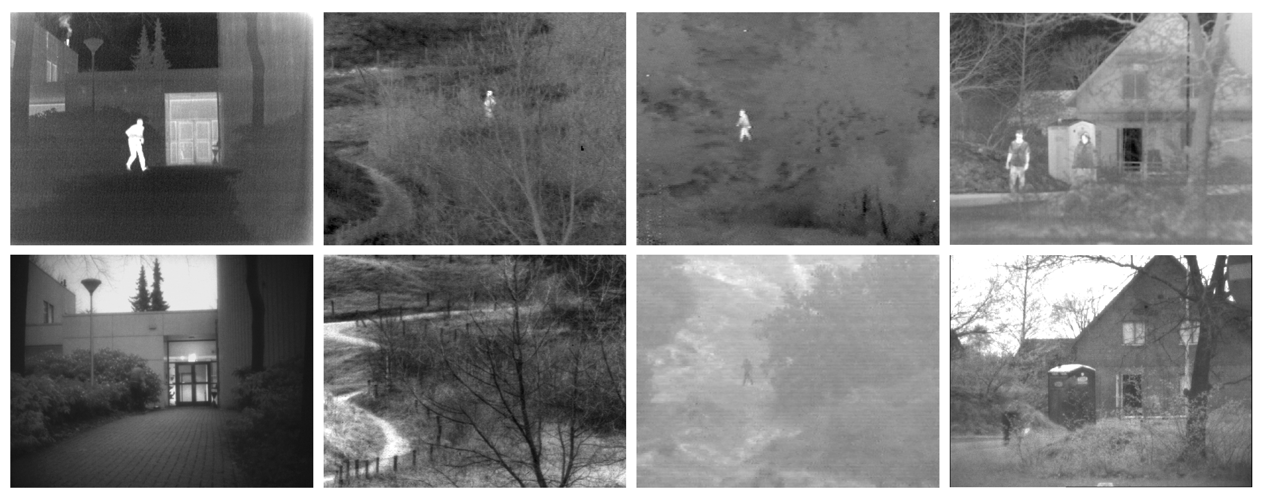
The TNO dataset [37] is one of the most commonly used datasets for IR and visible image fusion tasks. Most of the scenes in the dataset are military-related, including tanks, soldiers, fighter jets, jeeps, etc.

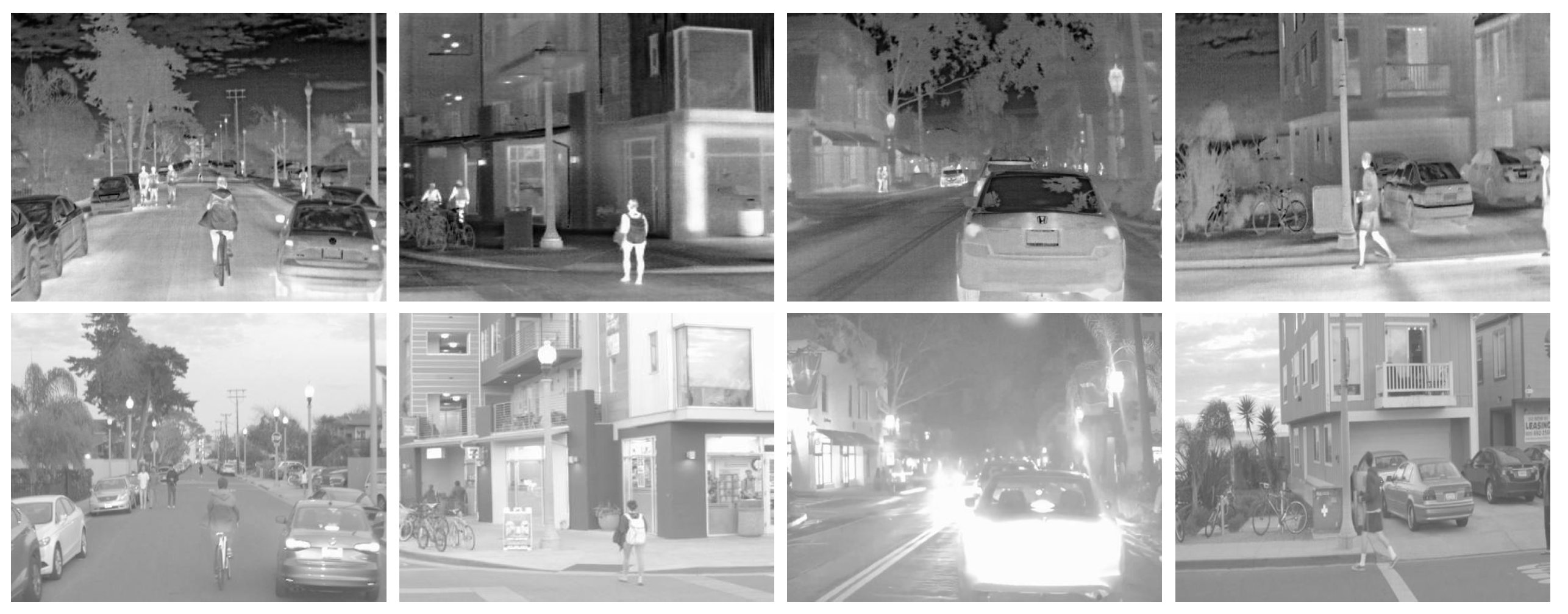
The RoadScene dataset (https://github.com/hanna-xu/RoadScene, accessed on 1 June 2023) is a dataset released by Xu et al. [38] based on FLIR videos that mainly includes rich scenes such as roads, vehicles, and pedestrians.

Figure 2 and Figure 3 show several examples of the TNO dataset and the RoadScene dataset.

2.4. Hainan Gibbon ($Nomascus$ $hainanus$) Dataset

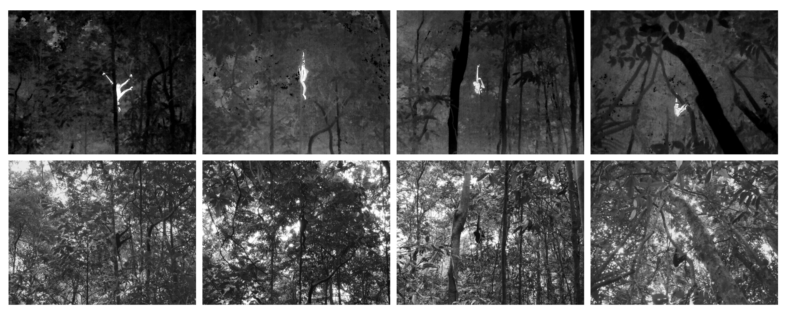
In order to verify the robustness of the proposed algorithm on different datasets, our team took a large number of IR and visible images of Hainan gibbons ($Nomascus$ $hainanus$) using a drone [39]. Hainan gibbons are the most endangered primates in the world and are in danger of extinction at any time [40]. The Hainan gibbon is listed as critically endangered by the International Union for Conservation of Nature Red List of Threatened Species [41]. At present, there are only 37 Hainan gibbons in the world, which are distributed in Bawangling National Nature Reserve in Changjiang Li Autonomous County, Hainan Province, China. Nonhuman primate species are our closest biological relatives, and they can provide insights into human evolution, biology, behavior, and the threat of emerging diseases [42]. Hainan gibbons live in foggy and complex tropical rainforests all year round [43]. It is difficult to capture useful information about the Hainan gibbons based on a single IR image or visible image. The fusion of IR and visible images can observe the movements and habitat of the Hainan gibbons and provide an important reference for wildlife protection. Figure 4 shows several examples of the Hainan gibbon dataset.

3. The Proposed Fusion Method

In order to better highlight salient objects in the source images, we propose an end-to-end salient residual Swin Transformer for IR and visible image fusion network, termed SDRSwin. The proposed fusion network is shown in Figure 5, and it includes an encoder, a residual dense fusion network (RDFN), and a decoder. The SDRSwin network is trained with a two-stage training approach. In the first stage of training, we use the $l_1$ loss function and the structural similarity loss to train an encoder–decoder network. In the second stage of training, we propose a novel salient loss function to train RDFN, which aims to guide the network to fuse the salient features of different modalities. The proposed salient loss function is presented in Section 3.2.2. In the fusion stage, the encoder first extracts the IR and visible features of the source images. Then, these features are fused through RDFN. At last, the fused features are rebuilt via the decoder to obtain the fused image.

3.1. The Architecture of the Proposed Method

3.1.1. Encoder and Decoder Networks

We use an encoder-and-decoder network based on residual Swin Transformers [20,21], aiming to obtain an encoder–decoder architecture with powerful feature extraction and reconstruction abilities. We assume that IR image $A\in {\mathbb{R}}^{H\times W\times C_{in}}$ and visible image $B\in {\mathbb{R}}^{H\times W\times C_{in}}$ are pre-registered images. In addition, H, W, and $C_{in}$ denote the length, width, and number of channels of the image, respectively. The encoder network includes a shallow feature extraction layer (SFEL) and three residual Swin Transformer layers (RSTLs), where SFEL is composed of a $1\times 1$ convolutional layer and a LayerNorm (LN) layer, and each RSTL consists of two successive Swin Transformer blocks (STBs). Figure 6 denotes the structure of RSTL. The decoder network consists of three RSTLs and a $1\times 1$ convolutional layer.

Firstly, an SFEL is used to extract the shallow features of A and B, and then the channel $C_{in}$ is transformed into C:

$$\begin{array}{c}\hfill {\Phi }_S^0=SFEL\left(S\right),S\in \left\{A,B\right\},\end{array}$$

(1)

where $SFEL\left(·\right)$ represents the shallow feature extraction operation. In our work, we set C to 96.

Secondly, the three RSTLs are utilized in the encoder to extract global and long-range semantic information:

$$\begin{array}{c}\hfill {\Phi }_S^m=ENCODE{R}_{RST{L}_m}\left({\Phi }_S^{m-1}\right)+{\Phi }_S^{m-1},m=1,2,3,\end{array}$$

(2)

$$\begin{array}{c}\hfill H_m,W_m,C_m=H,W,96,\end{array}$$

(3)

where $ENCODE{R}_{RST{L}_m}\left(·\right)$ indicates the m-th RSTL in the encoder, and $H_m$, $W_m$, and $C_m$ represent the length, width, and number of channels of the m-th RSTL’s features, respectively. With such a structural design, the global and long-range semantic features of IR and visible images are captured.

Thirdly, the RDFN is employed to fuse deep features of different modalities:

$$\begin{array}{c}\hfill {\Phi }_F^0=RDFN\left({\Phi }_A^3,{\Phi }_B^3\right),\end{array}$$

(4)

where $RDFN\left(·\right)$ represents the residual dense fusion network operation and ${\Phi }_F^0\in {\mathbb{R}}^{H\times W\times 96}$.

Finally, the fusion result is obtained through three RSTLs in the decoder and one convolutional layer:

$$\begin{array}{c}\hfill {\Phi }_F^n=DECODE{R}_{RST{L}_n}\left({\Phi }_F^{n-1}\right)+{\Phi }_F^{n-1},n=1,2,3,\end{array}$$

(5)

$$\begin{array}{c}\hfill H_n,W_n,C_n=H,W,96,\end{array}$$

(6)

$$\begin{array}{c}\hfill F=CONV\left({\Phi }_F^3\right),\end{array}$$

(7)

where $DECODE{R}_{RST{L}_n}\left(·\right)$ represents the n-th RSTL in the decoder, $CONV$ denotes a $1\times 1$ convolutional layer, and F indicates the fused image.

3.1.2. Swin Transformer Block (STB)

The Swin Transformer block (STB) is a multi-headed self-attention Transformer layer that is based on local attention and shifted window mechanisms [34]. Each STB consists of a multi-head self-attention (MSA) layer, two layer normalization (LN) layers, and a multi-layer perceptron (MLP) layer. MSA contains windows multi-head self-attention (W-MSA) and shifted windows multi-head self-attention (SW-MSA). A LN layer is utilized before each MSA and each MLP, and a residual connection is applied after each layer. The architecture of two successive Swin Transformer blocks is shown in Figure 7, and it is calculated as:

$$\begin{array}{c}\hfill \begin{array}{c}X=\mathrm{W}\text{-}\mathrm{MSA}\left(\mathrm{LN}\left(X\right)\right)+X\hfill \\ X=\mathrm{MLP}\left(\mathrm{LN}\left(X\right)\right)+X\hfill \\ X=\mathrm{SW}\text{-}\mathrm{MSA}\left(\mathrm{LN}\left(X\right)\right)+X\hfill \\ O=\mathrm{MLP}\left(\mathrm{LN}\left(X\right)\right)+X\hfill \end{array}\end{array}$$

(8)

where X denotes the local window of the input and O represents the output.

Assume that the size of the input image is $H\times W\times C$. Firstly, the input image is segmented into non-overlapping $M\times M$ local windows and further reshaped into $\frac{HW}{M^2}\times M^2\times C$, where $\frac{HW}{M^2}$ represents the total number of windows. Secondly, the corresponding self-attention mechanism is implemented in each corresponding window. In addition, the query Q, key K, and value V matrices are calculated as:

$$\begin{array}{c}\hfill Q=X{W}^Q,K=X{W}^K,V=X{W}^V,\end{array}$$

(9)

where X stands for the input local window feature, and $W^Q$, $W^K$, and $W^V$ are learnable projection weight matrices that are shared across various windows.

The attention mechanism of matrices is calculated as:

$$\begin{array}{c}\hfill \mathrm{Attention}\left(Q,K,V\right)=\mathrm{SoftMax}\left(\frac{Q{K}^T}{\sqrt{d}}+B\right)V,\end{array}$$

(10)

where B is the learnable relative positional encoding and d is the dimension of keys.

3.1.3. Residual Dense Fusion Network (RDFN)

In order to avoid the limitations of the hand-designed fusion scheme, a residual dense fusion network (RDFN) is utilized to detect and fuse the salient features of IR and visible images. The RDFN contains four convolutional layers (Conv1, Conv2, Conv3, Conv4) and three convolutional blocks (ConvBlock1, ConvBlock2, ConvBlock3). In particular, a convolutional block consists of two convolutional layers. The RDFN captures and fuses the salient features of different modalities through residual connections [44], convolutional blocks [45], and skip connections. The architecture and network parameters of the RDFN are shown in Figure 8 and

Table 1. The network settings of RDFN.

Layer	Kernel Size	Stride	Channel (Input)	Channel (Output)	Activation
Conv1	$3\times 3$	1	96	96	Relu
Conv2	$3\times 3$	1	96	96	Relu
Conv3	$3\times 3$	1	192	96	Relu
Conv4	$3\times 3$	1	96	1	Relu
ConvBlock1	$3\times 3$	1	192	96	Relu
	$1\times 1$	1	96	192	Relu
ConvBlock2	$3\times 3$	1	384	192	Relu
	$1\times 1$	1	192	96	Relu
ConvBlock3	$3\times 3$	1	480	240	Relu
	$1\times 1$	1	240	96	Relu

, respectively.

3.2. Two-Stage Training Strategy

The proposed approach adopts a two-stage training strategy, where the first stage is the training of the encoder–decoder network and the second stage is the training of the RDFN. The first stage of training aims to train a powerful encoder–decoder network to reconstruct the input image. The purpose of the second stage of training is to train a RDFN to fuse salient features.

3.2.1. Training of the Encoder–Decoder Network

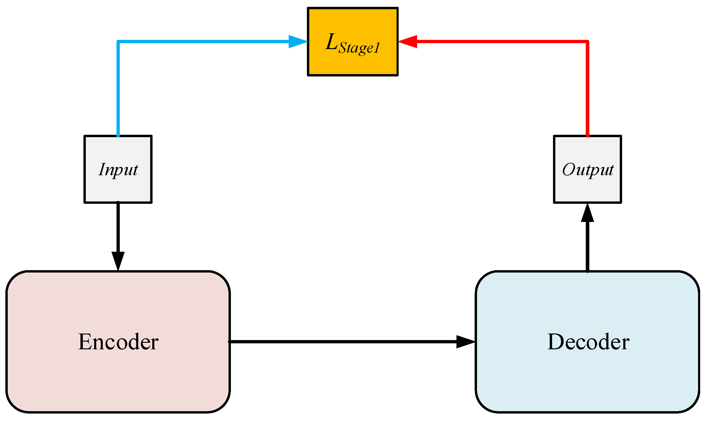
The first stage of training is shown in Figure 9, where we just consider encoder and decoder networks (the RDFN is discarded). The loss function $L_{stage1}$ of the first stage is calculated as:

$$\begin{array}{c}\hfill L_{stage1}=L_{l_1}+\lambda L_{ssim},\end{array}$$

(11)

where $L_{l_1}$ represents the $l_1$ loss function, $L_{ssim}$ indicates the structural similarity loss, and $\lambda$ stands for the trade-off between $L_{l_1}$ and $L_{ssim}$.

In addition, $L_{l_1}$ and $L_{ssim}$ are calculated as:

$$\begin{array}{c}\hfill L_{l_1}=\frac{1}{HW}\sum \left|Output-Input\right|,\end{array}$$

(12)

$$\begin{array}{c}\hfill L_{ssim}=1-\mathrm{SSIM}\left(Output,Input\right),\end{array}$$

(13)

where $Input$ denotes the input training image, $Output$ is the output image, H represents the height of the image, W indicates the width of the image, and $\mathrm{SSIM}\left(·\right)$ stands for the structural similarity measure [46]. On the one hand, a smaller $L_{l_1}$ indicates that the reconstructed image is more similar to the input image. On the other hand, a smaller $L_{ssim}$ means that the output image and input image are more similar in structure.

3.2.2. Training of the RDFN

In the process of fusion, the most critical problem is how to extract the salient targets in the IR image and the background detail regions in the visible image. The loss function determines the distribution ratio of IR and visible features in the fusion result. Therefore, in the second stage, we develop a novel salient loss function to guide the RDFN to fuse the salient targets in the IR image and the background detail regions in the visible image.

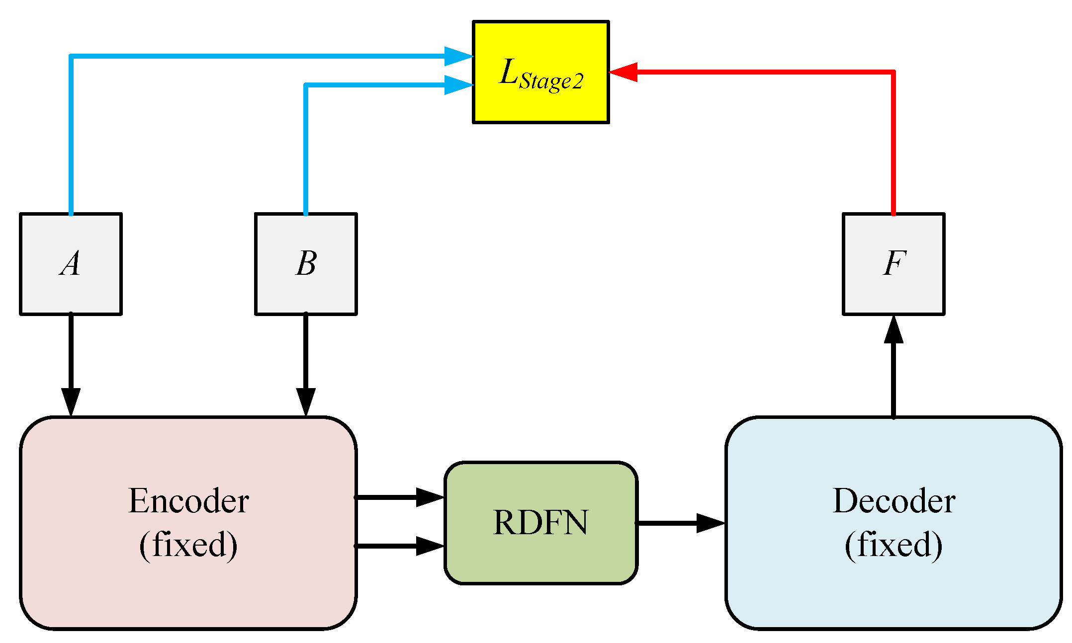
The second stage of training is shown in Figure 10, where A indicates an IR image, B is a visible image, and F denotes a fused image.

With the encoder and decoder fixed, the loss function $L_{stage2}$ of the second stage is calculated as:

$$\begin{array}{c}\hfill L_{stage2}=\left(2L_{salient\_ir}+L_{pixel\_ir}+L_{ssim\_ir}\right)+\left(L_{salient\_vis}+L_{pixel\_vis}+L_{ssim\_vis}\right).\end{array}$$

(14)

The loss function in the second stage consists of three loss functions: salient loss, pixel loss, and structural similarity loss. In the above equation, $L_{salient\_ir}$ and $L_{salient\_vis}$ represent IR and visible salient losses, respectively; $L_{pixel\_ir}$ and $L_{pixel\_vis}$ indicate IR and visible pixel losses, respectively; $L_{ssim\_ir}$ and $L_{ssim\_vis}$ denote IR and visible structural similarity losses, respectively.

The salient loss limits the fused image to have the same pixel intensity distribution as the desired image. $L_{salient\_ir}$ and $L_{salient\_vis}$ are, respectively, calculated as:

$$\begin{array}{c}\hfill L_{salient\_ir}=\frac{1}{HW}{∥A\circ \left(F-A\right)∥}_1,\end{array}$$

(15)

$$\begin{array}{c}\hfill L_{salient\_vis}=\frac{1}{HW}{∥B\circ \left(F-B\right)∥}_1,\end{array}$$

(16)

where H and W represent the height and width of the image, respectively; ∘ denotes the elementwise multiplication; and ${∥·∥}_1$ stands for the $l_1$-norm. With such a loss function design, the network can extract salient objects in the IR image and background detail regions in the visible image.

The pixel loss calculates the distance between the fused image and the input image, with the purpose of making the fused image more similar to the input image at the pixel level. $L_{pixel\_ir}$ and $L_{pixel\_vis}$ are, respectively, computed as:

$$\begin{array}{c}\hfill L_{pixel\_ir}={∥F-A∥}_F^2,\end{array}$$

(17)

$$\begin{array}{c}\hfill L_{pixel\_vis}={∥F-B∥}_F^2,\end{array}$$

(18)

where ${∥·∥}_F^2$ stands for the Frobenius norm.

The structural similarity loss calculates the structural similarity between the fused image and the input image, with the goal of making the fused image more similar to the input image in structure. $L_{ssim\_ir}$ and $L_{ssim\_vis}$ are, respectively, calculated as:

$$\begin{array}{c}\hfill L_{ssim\_ir}=1-\mathrm{SSIM}\left(F,A\right),\end{array}$$

(19)

$$\begin{array}{c}\hfill L_{ssim\_vis}=1-\mathrm{SSIM}\left(F,B\right).\end{array}$$

(20)

Algorithm 1 provides an overview of the key phases of the proposed algorithm.

Algorithm 1 Proposed infrared and visible image fusion algorithm

Training stage

Part 1: The first-stage training

1 Initialize the encoder and decoder networks of SDRSwin;

2 Train the parameters of encoder and decoder networks through minimizing $L_{stage1}$

defined in Equations (11)–(13);

Part 2: The second-stage training

3 Initialize the RDFN;

4 Train the parameters of the RDFN through minimizing $L_{stage2}$ defined in

Equations (14)–(20).

Testing (fusion) stage

Part 1: Encoder

1. Feed infrared image A and visible image B into an SFEL and three RSTLs to obtain

the infrared feature ${\Phi }_A^3$ and visible feature ${\Phi }_B^3$ according to Equations (1)–(3);

Part 2: RDFN

2. Feed infrared feature ${\Phi }_A^3$ and visible feature ${\Phi }_B^3$ to RDFN to generate the fused

feature ${\Phi }_F^0$ according to Equation (4);

Part 3: Decoder

3. Feed the fused feature ${\Phi }_F^0$ into three RSTLs and a convolutional layer to obtain

the fused image F according to Equations (5)–(7).

4. Experimental Results

The first part describes the experimental settings. The second part introduces subjective and objective evaluation metrics. The third part shows several ablation studies. The last part is three comparative experiments on the TNO, RoadScene, and Hainan gibbon datasets.

4.1. Experimental Settings

MS-COCO [47] is a dataset based on natural images, and KAIST [48] is a dataset based on infrared and visible images. The first stage of training aims to train a powerful encoder–decoder network to reconstruct the input image. The purpose of the second stage of training is to train a RDFN to fuse salient features.

In the first-stage training, we trained the encoder–decoder network by using 80,000 images from the MS-COCO dataset, and each image was converted to a $224\times 224$ grayscale image. We set the patch size and sliding window size to $1\times 1$ and $7\times 7$, respectively. Furthermore, we selected Adam as the optimizer and set the following parameters: $1\times {10}^{-5}$ for learning rate, 4 for batch size, and 3 for epoch. The head numbers of the three RSTLs in the encoder were set to 1, 2, and 4, respectively. The head numbers of the three RSTLs in the decoder were also set to 1, 2, and 4, respectively. In addition, $\lambda$ was specifically analyzed in the ablation study.

In the second-stage training, we used 50,000 pairs of images from the KAIST dataset to train the RDFN, and each image was converted to a $224\times 224$ grayscale image. In addition, we selected Adam as the optimizer and set the learning rate, batch size, and epoch to $1\times {10}^{-5}$, 4, and 3, respectively.

In the fusion stage, we converted the grayscale range of test images to −1 and 1 and applied the sliding window $224\times 224$ to partition them into several patches, where the value of the invalid region is filled with 0. After the combination of each patch pair, we conducted the reverse operation according to the previous partition order to obtain the fusion image. The experimental environments of our method were Intel Core i7 13700KF, NVIDIA GeForce RTX 4090 24 GB and PyTorch.

4.2. Evaluation Metrics

The validity of the proposed approach is assessed in terms of both subjective visual evaluation and objective evaluation metrics.

Subjective evaluation is the evaluation of the visual effect of the fused image by human eyes, including color, brightness, definition, contrast, noise, fidelity, etc. The subjective evaluation is essentially to judge whether the fused image gives a satisfactory feeling.

Objective evaluation is a comprehensive assessment of the fusion performance of algorithms through various objective evaluation metrics. We selected eight important and common evaluation metrics:

• Entropy ($EN$) [49]: $EN$ is an information theory-based evaluation metric that calculates the degree of information contained in the fused image;
• Standard deviation ($SD$) [50]: $SD$ reflects the contrast and distribution of the fused image;
• Normalized mutual information metric $Q_{MI}$ [51]: $Q_{MI}$ measures normalized mutual information between the fused image and the source images;
• Nonlinear correlation information entropy metric $Q_{NCIE}$ [52]: $Q_{NCIE}$ calculates the nonlinear correlation information entropy of the fused image;
• Phase-congruency-based metric $Q_P$ [53]: $Q_P$ measures the extent to which salient features in the source images are transferred to the fused image, and it is based on the absolute measure of image features;
• Chen–Varshney metric $Q_{CV}$ [54]: $Q_{CV}$ provides a fusion metric of a human vision system that can fit the results of human visual inspection well;
• Visual information fidelity ($VIF$) [55]: $VIF$ measures the fidelity of the fused image;
• Mutual information ($MI$) [56]: $MI$ computes the amount of information transferred from the source images to the fused image.

In all the above metrics, except $Q_{CV}$, the higher the value of the metrics, the better the fusion performance. The smaller the value of $Q_{CV}$, the better the fusion performance. In objective evaluation, the more optimal the values of a method, the stronger the fusion performance of the method.

4.3. Ablation Study

In this part, we carried out several ablation studies to verify the validity of the proposed method. We used the above-mentioned 21 pairs of images from the TNO dataset as test images, and the average of eight objective evaluation metrics as reference standards.

4.3.1. Parameter $\lambda$ Ablation Study in Loss Function in the First Stage

In the first stage of training, due to the different orders of magnitude of $L_{ssim}$ and $L_{pixel}$, we set the trade-off parameter $\lambda$ as 1, 10, 100, 1000, and 10,000, respectively.

Table 2. The average values of different $\lambda$ objective evaluation metrics.

$\mathit{\lambda }$	$\mathit{EN}$	$\mathit{SD}$	${\mathit{Q}}_{\mathit{MI}}$	${\mathit{Q}}_{\mathit{NCIE}}$	${\mathit{Q}}_{\mathit{P}}$	${\mathit{Q}}_{\mathit{CV}}$	$\mathit{VIF}$	$\mathit{MI}$
1	6.9137	42.6050	0.4842	0.8081	0.3168	335.8123	0.9716	3.2746
10	6.8700	41.5785	0.4797	0.8080	0.3110	333.8100	0.9598	3.2347
100	6.9253	42.8145	0.4716	0.8078	0.3086	325.3314	0.9667	3.1926
1000	6.8763	42.1298	0.4759	0.8079	0.3111	322.1715	0.9679	3.2112
10,000	6.8847	42.0794	0.4823	0.8080	0.3132	341.2470	0.9706	3.2575

shows the average values of different $\lambda$ objective evaluation metrics, where the best values are indicated in red font. The model obtains the most optimal values when $\lambda =1$. Therefore, we chose $\lambda =1$ as the trade-off parameter in the following experiments.

4.3.2. Residual Connections Ablation Study

We verified the impact of residual connections on the fusion model. The without residual connections method means that residual connections are removed from all RSTLs, and all other parameters are set the same.

Table 3. The average values of objective evaluation metrics for without and with residual connections methods.

Method	$\mathit{EN}$	$\mathit{SD}$	${\mathit{Q}}_{\mathit{MI}}$	${\mathit{Q}}_{\mathit{NCIE}}$	${\mathit{Q}}_{\mathit{P}}$	${\mathit{Q}}_{\mathit{CV}}$	$\mathit{VIF}$	$\mathit{MI}$
Without Residual	6.9275	41.7175	0.4564	0.8074	0.2975	339.8872	0.9473	3.0982
Our	6.9137	42.6050	0.4842	0.8081	0.3168	335.8123	0.9716	3.2746

presents the average values of objective evaluation metrics without and with residual connections, and we notice that the model with residual connections is obviously better than the model without residual connections, because residual connections preserve more critical information from the previous layer.

4.3.3. Salient Loss Function Ablation Study

In this part, we analyzed the impact of the salient loss function in the second stage of training on the fusion performance. We performed an ablation study to test the validity of the salient loss function. We trained a network without salient loss in the second stage, and the loss function is defined as follows:

$$\begin{array}{c}\hfill L_{without}=\left(L_{pixel\_ir}+L_{ssim\_ir}\right)+\left(L_{pixel\_vis}+L_{ssim\_vis}\right).\end{array}$$

(21)

Table 4. The average values of objective evaluation metrics for without and with salient losses methods.

Method	$\mathit{EN}$	$\mathit{SD}$	${\mathit{Q}}_{\mathit{MI}}$	${\mathit{Q}}_{\mathit{NCIE}}$	${\mathit{Q}}_{\mathit{P}}$	${\mathit{Q}}_{\mathit{CV}}$	$\mathit{VIF}$	$\mathit{MI}$
Without salient loss	6.8863	38.5237	0.3762	0.8067	0.2838	662.0475	0.8492	2.5793
Our	6.9137	42.6050	0.4842	0.8081	0.3168	335.8123	0.9716	3.2746

presents the average values of objective evaluation metrics for the networks without and with salient losses. We observe that the fusion performance of the network with salient loss is significantly better than that of the network without salient loss, demonstrating that the proposed salient loss function can guide the network to better fuse the salient features.

4.4. The Three Comparative Experiments

In this section, we used 21 pairs of images from the TNO dataset, 44 pairs of images from the RoadScene dataset, and 21 pairs of images from the Hainan gibbon dataset as test images. We selected 21 classical and state-of-the-art competitive algorithms for comparison. The 21 comparison methods mainly contain five types, i.e., MST methods (RP [6], DWT [7], CVT [8], DTCWT [9], MSVD [10], LatLRR [11], MLGCF [12]), SR methods (JSM [14]), saliency methods (TSSD [15], CSF [17]), optimization-based methods (GTF [18], DRTV [19]), and deep learning methods (VggML [24], ResNet-ZCA [26], DenseFuse [28], FusionGAN [23], GANMcC [30], U2Fusion [31], RFN-Nest [22], DRF [29], SwinFuse [21]). All parameters of the comparison approaches are the default values provided by the corresponding authors.

4.4.1. The Experiment on the TNO Dataset

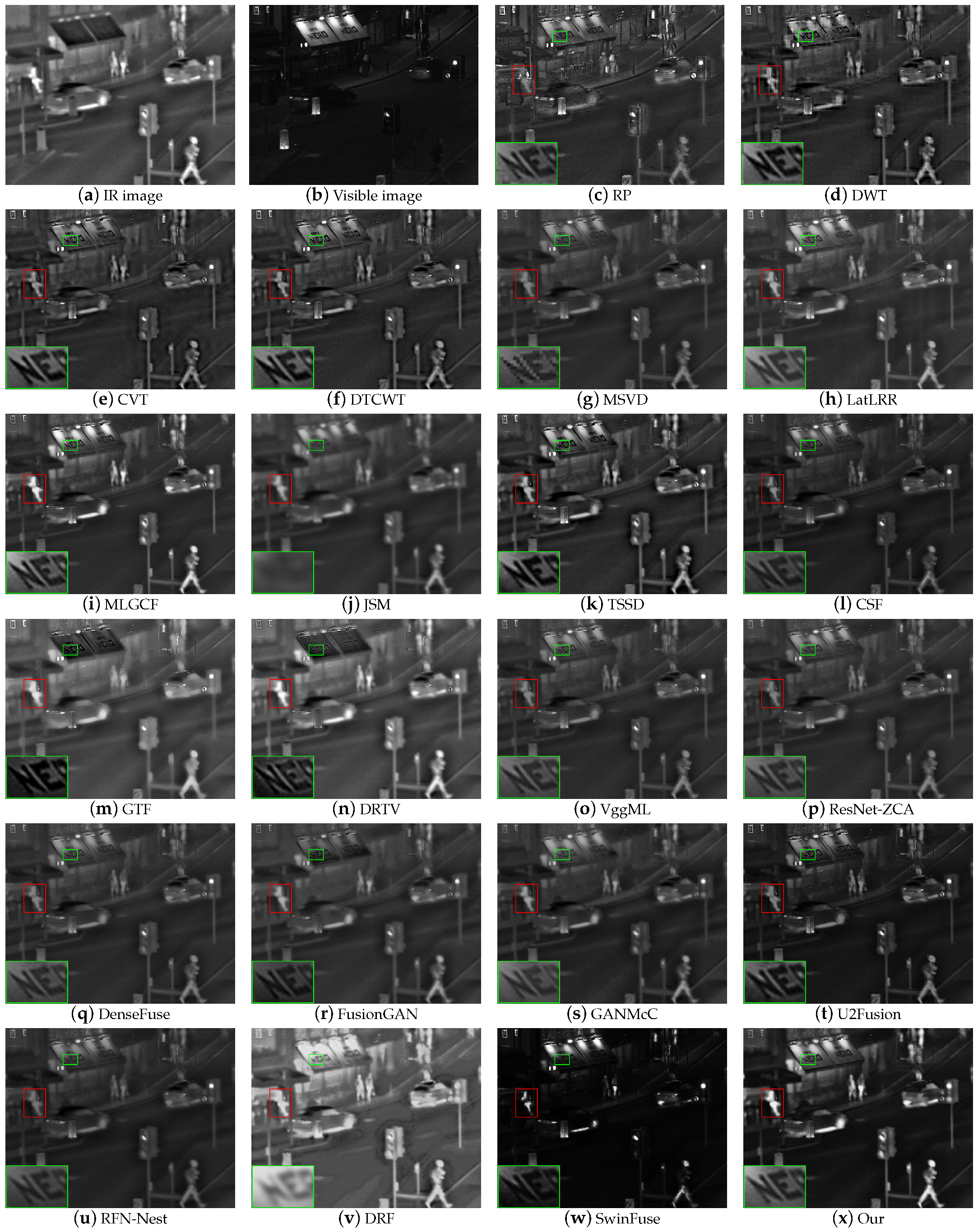
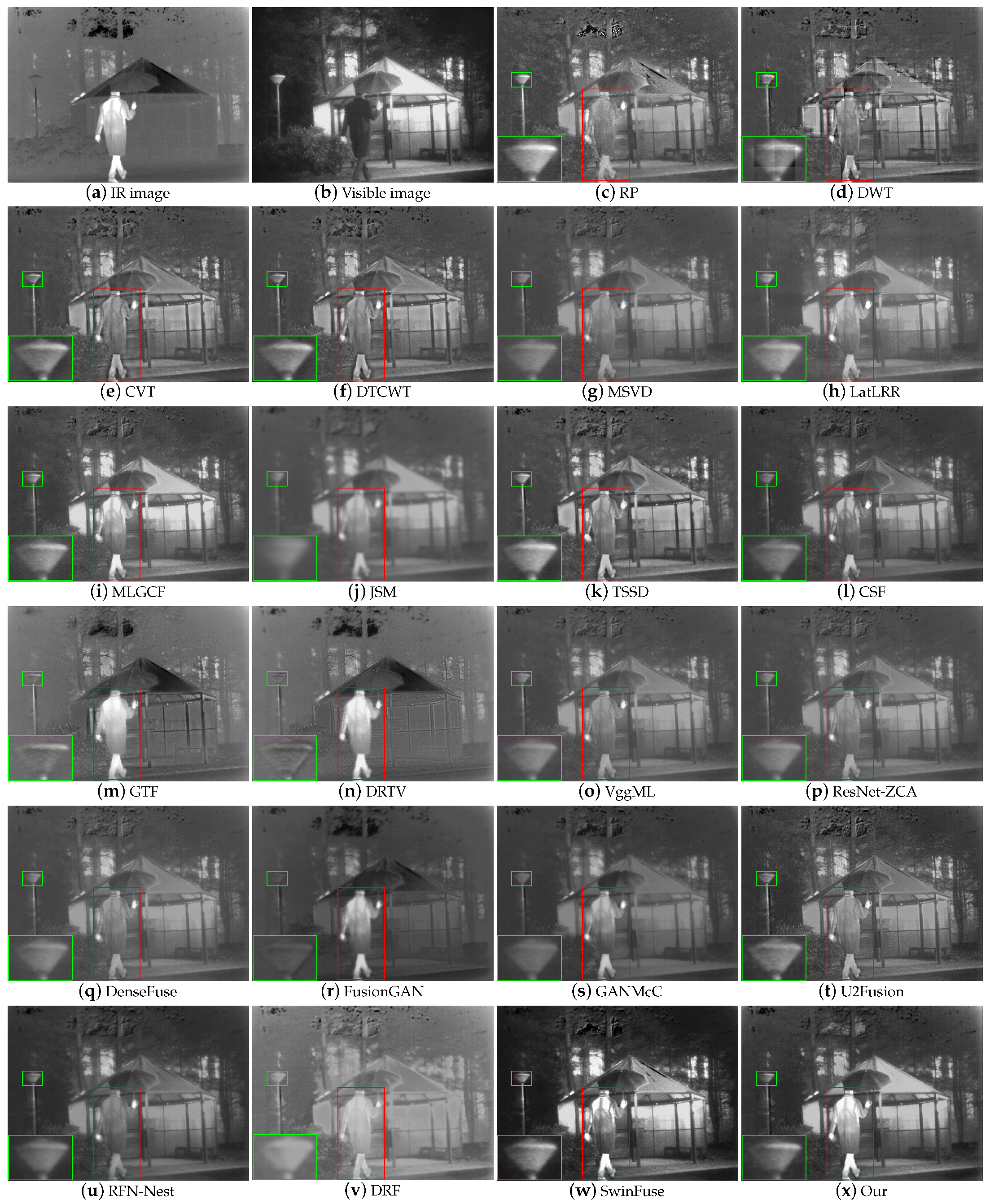
Figure 11, Figure 12 and Figure 13 exhibit several representative fusion examples. Some parts of the images are enlarged by rectangular boxes for a better visual effect. Figure 11 shows the scene on the road at night. The IR image shows information about thermal radiation objects at night-time, such as pedestrians, cars, and street lights. Due to the night scene, the visible image can only capture the details of the panels of the store with high brightness. The desired fusion effect in this case is to maintain the high luminance of the thermal radiation object information and simultaneously keep the clarity of the store panels’ details. The RP, DWT, and CVT methods introduce some artifacts around pedestrians (see the red boxes in Figure 11c–e). The pedestrians in the DTCWT method suffer from low brightness and contrast (as shown in the man in Figure 11f). The MSVD result brings in obvious noise in the store panels (see Figure 11g). The pedestrians in the LatLRR technique have low luminance (as shown in the man in Figure 11h), and this result produces some artifacts during the fusion process (see the road in Figure 11h). The MLGCF approach obtains a great fusion result. The fused image of the JSM algorithm is significantly blurred (as shown in Figure 11j). In the saliency-based fusion approaches, the IR targets in the TSSD and CSF methods have low luminance (see the red boxes in Figure 11k,l). The panels in the GTF and DRTV methods introduce an excessive infrared spectrum, resulting in a lack of details in the panels (see green boxes in Figure 11m,n). In this example, most of the visible information around the panels is desired. In deep-learning-based methods, the pedestrians in the red boxes in VggML, ResNet-ZCA, DenseFuse, FusionGAN, GANMcC, U2Fusion, and RFN-Nest approaches suffer from low luminance and contrast (as shown in the man in Figure 11o–u). The DRF-based method appears overexposed, and the panels are fuzzy (see Figure 11v). The SwinFuse is a non-end-to-end fusion approach that employs a fusion strategy based on an artificially designed $l_1$-norm. The SwinFuse method appears excessively dark because the $l_1$-norm fusion rule does not integrate infrared and visible features well (see Figure 11w). Compared with other methods, our method obtains a higher brightness and contrast of the IR saliency targets (as shown in the man in Figure 11x), and clearer panel details (as shown in the store panels in Figure 11x).

Figure 12 and Figure 13 show more fusion results.

Table 5. The average values of different methods on the TNO dataset.

Method	$\mathit{EN}$	$\mathit{SD}$	${\mathit{Q}}_{\mathit{MI}}$	${\mathit{Q}}_{\mathit{NCIE}}$	${\mathit{Q}}_{\mathit{P}}$	${\mathit{Q}}_{\mathit{CV}}$	$\mathit{VIF}$	$\mathit{MI}$
RP	6.5014	27.8622	0.2398	0.8037	0.2527	682.3019	0.7036	1.5768
DWT	6.5012	27.4182	0.2495	0.8038	0.2289	501.7177	0.6033	1.6416
CVT	6.4314	26.0457	0.2407	0.8037	0.2585	506.9577	0.5996	1.5757
DTCWT	6.3903	25.6292	0.2511	0.8038	0.2798	519.5448	0.6317	1.6474
MSVD	6.1927	22.7202	0.2961	0.8043	0.2239	510.2300	0.6079	1.9090
LatLRR	6.3574	25.8487	0.2839	0.8041	0.2635	434.5201	0.6436	1.8453
MLGCF	6.6412	34.3708	0.3391	0.8052	0.2891	402.9804	0.7467	2.2662
JSM	6.1733	25.0041	0.2895	0.8041	0.0558	580.3658	0.3117	1.8494
TSSD	6.5260	28.2417	0.2529	0.8038	0.3021	414.0477	0.7291	1.6667
CSF	6.7905	35.7161	0.2975	0.8045	0.2481	490.5935	0.7458	2.0084
GTF	6.6353	31.5791	0.3637	0.8061	0.2003	1281.2336	0.5656	2.4225
DRTV	6.3210	30.8169	0.3899	0.8069	0.0896	1568.6859	0.6741	2.5746
VggML	6.1819	22.6981	0.3290	0.8047	0.2893	478.8354	0.6127	2.1124
ResNet-ZCA	6.1953	22.9400	0.3167	0.8046	0.2885	461.4566	0.6141	2.0328
DenseFuse	6.1740	22.5463	0.3340	0.8048	0.2861	471.9678	0.6088	2.1434
FusionGAN	6.3629	26.0676	0.3476	0.8052	0.0989	1061.5684	0.6525	2.2570
GANMcC	6.5422	30.2862	0.3388	0.8048	0.2295	642.7662	0.6646	2.2414
U2Fusion	6.7571	31.7084	0.2691	0.8040	0.2604	619.1068	0.7514	1.8045
RFN-Nest	6.8413	35.2704	0.3007	0.8045	0.2374	534.2482	0.7926	2.0351
DRF	6.7187	30.7325	0.2641	0.8040	0.0886	1122.9130	0.6315	1.7626
SwinFuse	6.8820	46.9457	0.3549	0.8056	0.2908	433.7429	0.8299	2.3907
Our	6.9137	42.6050	0.4842	0.8081	0.3168	335.8123	0.9716	3.2746

exhibits the average values of different objective evaluation metrics on the TNO dataset, where the best values are indicated in red font. Table 5 displays that our approach achieves optimal results in all objective evaluation metrics except $SD$, demonstrating that our approach has a stronger fusion performance than the other 21 comparison approaches.

4.4.2. The Experiment on the Roadscene Dataset

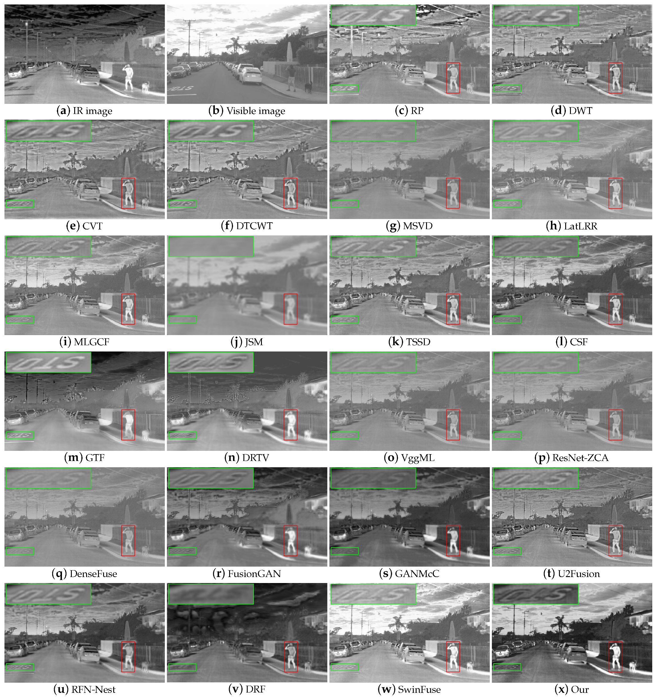
In this section, we verified the effectiveness of the proposed algorithm by employing the RoadScene dataset. We used 44 pairs of images from the RoadScene dataset as test images. Figure 14, Figure 15 and Figure 16 show several representative examples. Figure 14 depicts a person waiting on the roadside. The pedestrian and vehicle have high brightness in the IR image, and the visible image provides clearer background details. The fonts on the walls in the RP and MSVD methods are obviously blurred (see the green boxes in Figure 14c,g). The DWT-based approach introduces some noticeable noise around the vehicle (see the vehicle in Figure 14d). The results of CVT, DTCWT, and MLGCF are alike, and the IR targets in their results lack brightness (see the red boxes in Figure 14e,f,i). The pedestrians in the LatLRR method suffer from weak luminance and contrast (as shown by the man in Figure 14h). The JSM approach obtains a low fusion performance because its fusion result is fuzzy (see Figure 14j). In the saliency-based methods, the fonts in the wall of the TSSD approach are unclear (see the wall in Figure 14k). The fonts on the wall in the CSF approach bring in an excessive IR spectrum, leading to unnatural visual perception (see green boxes in Figure 14l). In this case, most of the visible details on the walls are desired. The GTF and DRTV methods achieve poor fusion results because of the introduction of obvious artifacts (see green boxes in Figure 14m,n). The fonts on the walls in the VggML, ResNet-ZCA, and DenseFuse approaches are significantly blurred (see the green boxes in Figure 14o–q). The pedestrian, vehicle, and trees in the FusionGAN method are fuzzy (as shown on the wall in Figure 14r). The GANMcC, U2Fusion, and RFN-Nest methods obtain a good fusion performance, but their IR targets lack some brightness (as shown in the man in Figure 14s–u). The DRF-based method achieves high luminance for the pedestrian and vehicle, but the background details are blurred, leading to an unnatural visual effect (as shown on the wall in Figure 14v). The upper-left tree in the SwinFuse method introduces a number of undesired little black dots, leading to an unnatural visual experience. In addition, the contrast in the fusion result of SwinFuse is low, which makes it difficult to highlight the targets well (see Figure 14w). Our approach highlights the brightness of the pedestrian and vehicle (as shown in the man in Figure 14x) and simultaneously maintains the details of the fonts on the walls well (see the green box in Figure 14x). As a result, our approach achieves a more natural visual experience and higher fusion performance.

In addition, Figure 15 and Figure 16 show more examples.

Table 6. The average values of different methods on the RoadScene dataset.

Method	$\mathit{EN}$	$\mathit{SD}$	${\mathit{Q}}_{\mathit{MI}}$	${\mathit{Q}}_{\mathit{NCIE}}$	${\mathit{Q}}_{\mathit{P}}$	${\mathit{Q}}_{\mathit{CV}}$	$\mathit{VIF}$	$\mathit{MI}$
RP	7.1424	39.2232	0.3251	0.8056	0.3684	1101.3929	0.7412	2.3478
DWT	7.1186	37.5085	0.3373	0.8058	0.3266	769.0781	0.6480	2.4328
CVT	7.0930	36.4588	0.3093	0.8053	0.3523	982.3925	0.6278	2.2247
DTCWT	7.0352	35.6115	0.3219	0.8055	0.3255	800.1602	0.6429	2.3057
MSVD	6.8257	31.7375	0.3831	0.8064	0.3122	808.7879	0.6795	2.7014
LatLRR	6.9070	34.3897	0.3680	0.8061	0.3481	814.2121	0.6770	2.6127
MLGCF	7.1553	39.3276	0.4073	0.8075	0.3732	795.6147	0.7648	2.9505
JSM	6.7059	31.2440	0.3430	0.8054	0.0789	752.1129	0.3029	2.3850
TSSD	7.1486	38.4876	0.3374	0.8058	0.3952	877.1808	0.7537	2.4365
CSF	7.3758	46.2558	0.3929	0.8070	0.3727	772.7454	0.7734	2.8790
GTF	7.4665	51.8793	0.4476	0.8084	0.2495	1595.9816	0.6061	3.3066
DRTV	6.4458	46.9789	0.4534	0.8082	0.1313	1672.9384	0.6636	3.1251
VggML	6.8143	31.6182	0.4164	0.8071	0.4017	791.5175	0.6854	2.9376
ResNet-ZCA	6.8117	31.5816	0.4150	0.8071	0.3964	798.9765	0.6815	2.9266
DenseFuse	6.8046	31.4389	0.4186	0.8071	0.3948	795.7429	0.6796	2.9503
FusionGAN	7.0392	38.1160	0.3889	0.8068	0.1387	1138.3050	0.5913	2.7851
GANMcC	7.1712	41.6191	0.3958	0.8066	0.3029	943.6773	0.6829	2.8421
U2Fusion	7.2495	41.9339	0.3845	0.8069	0.3939	859.1278	0.7305	2.8016
RFN-Nest	7.3188	44.7048	0.3824	0.8065	0.2648	981.0049	0.7396	2.7822
DRF	7.3031	47.6624	0.3683	0.8063	0.1138	1668.1819	0.4650	2.6812
SwinFuse	7.5148	57.7277	0.4264	0.8079	0.3883	612.9746	0.8218	3.1559
Our	7.4873	56.9426	0.5555	0.8112	0.3964	493.1310	0.9583	4.0885

exhibits the average values of different objective evaluation metrics on the RoadScene dataset, where the best values are indicated in red font. The proposed method achieved five best values ($Q_{MI}$, $Q_{NCIE}$, $Q_{CV}$, $VIF$, $MI$) and three second-best values ($EN$, $SD$, $Q_P$). The fusion performance of the proposed approach is significantly superior to the other 21 comparative approaches.

4.4.3. The Experiment on the Hainan Gibbon Dataset

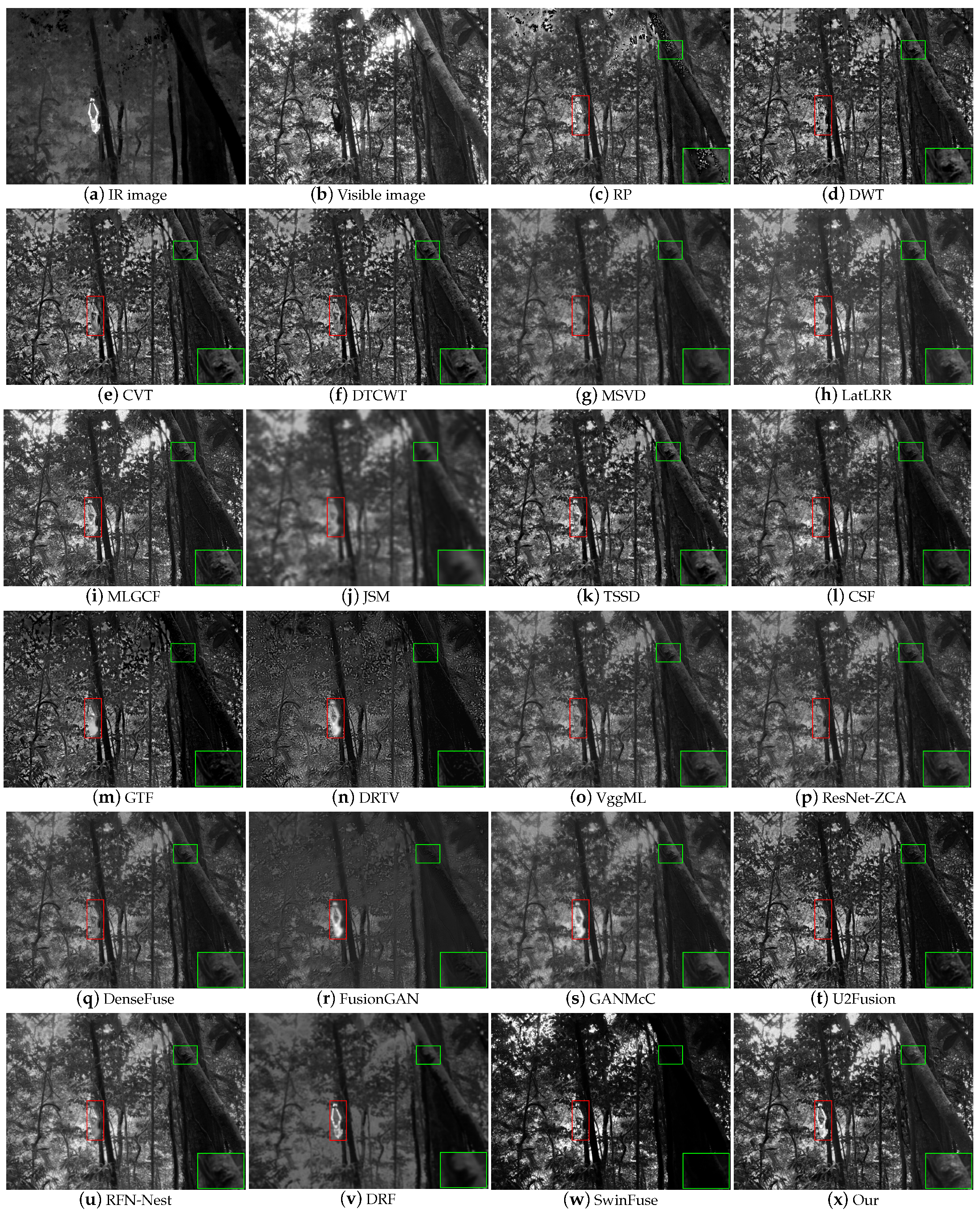
In this section, we used 21 pairs of images from the Hainan gibbon dataset as test images. Figure 17, Figure 18 and Figure 19 present several representative Hainan gibbon image fusion examples. Figure 17 depicts the scene of a gibbon preparing to jump in the tropical rainforest. The IR image accurately locates the position of the gibbon, but the tropical rainforest in the background is blurred. The visible image can hardly locate the position of the gibbon, but there are clear details of the tropical rainforest. The fusion of IR and visible images can be used to observe the movements and habitat of gibbons, providing an important reference for the protection of endangered animals. In RP, DWT, CVT, and DTCWT approaches, the gibbons are dim, and their results make it difficult to locate the position of the gibbons (see the gibbons in Figure 17c–f). In the MSVD, LatLRR, and JSM techniques, the tropical rainforests are fuzzy (see tropical rainforests in Figure 17g,h,j). Although the MLGCF approach achieves a relatively good fusion effect, the brightness of the gibbon in the fusion result is relatively low (see the thermal radiation target in Figure 17i). In the saliency-based scheme, the brightness of the gibbon in the TSSD and CSF schemes is similar to the background brightness, which makes it difficult to find the position of the gibbon (see the gibbons in Figure 17k,l). In addition, the GTF and DRTV approaches extract too much of the infrared spectrum, resulting in the loss of a large amount of tropical rainforest details (as shown in the background areas in Figure 17m,n). Among the deep-learning-based approaches, the gibbons in VggML, ResNet-ZCA, DenseFuse, U2Fusion, and RFN-Nest approaches have low brightness and contrast, making it difficult to discover the location of the gibbon (as shown in the red boxes in Figure 17o,p,q,t,u). Although the gibbons in FusionGAN, GANMCC, and DRF approaches have relatively high brightness and contrast, the backgrounds have lost a lot of details (see Figure 17r,s,v). The Hainan gibbon in the SwinFuse method is almost invisible, and the rainforest in the method loses a great number of details (see Figure 17w). The proposed method has a bright gibbon and a clear tropical rainforest background (see the red and green boxes in Figure 17x). Our method can easily locate the position of gibbons and observe their habitat.

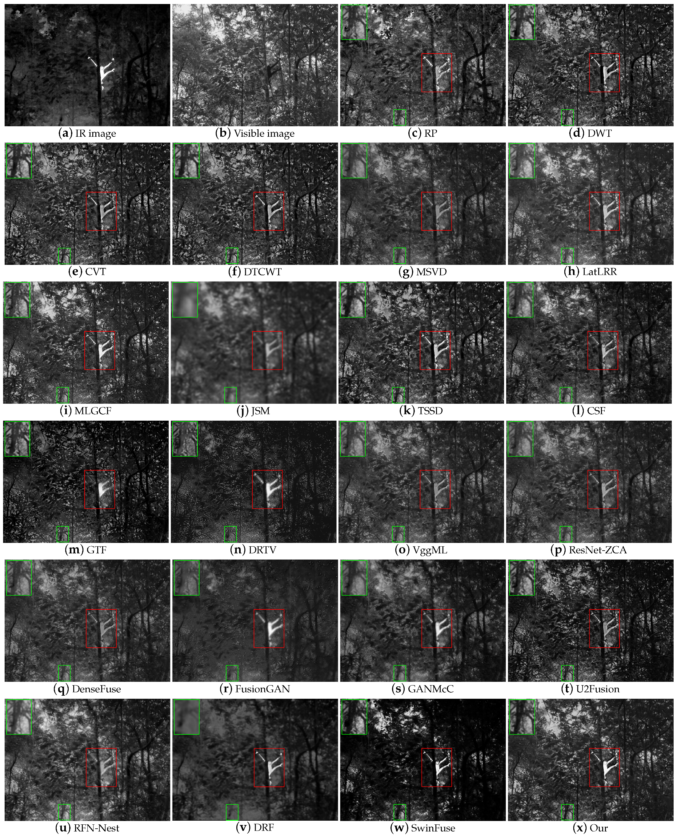
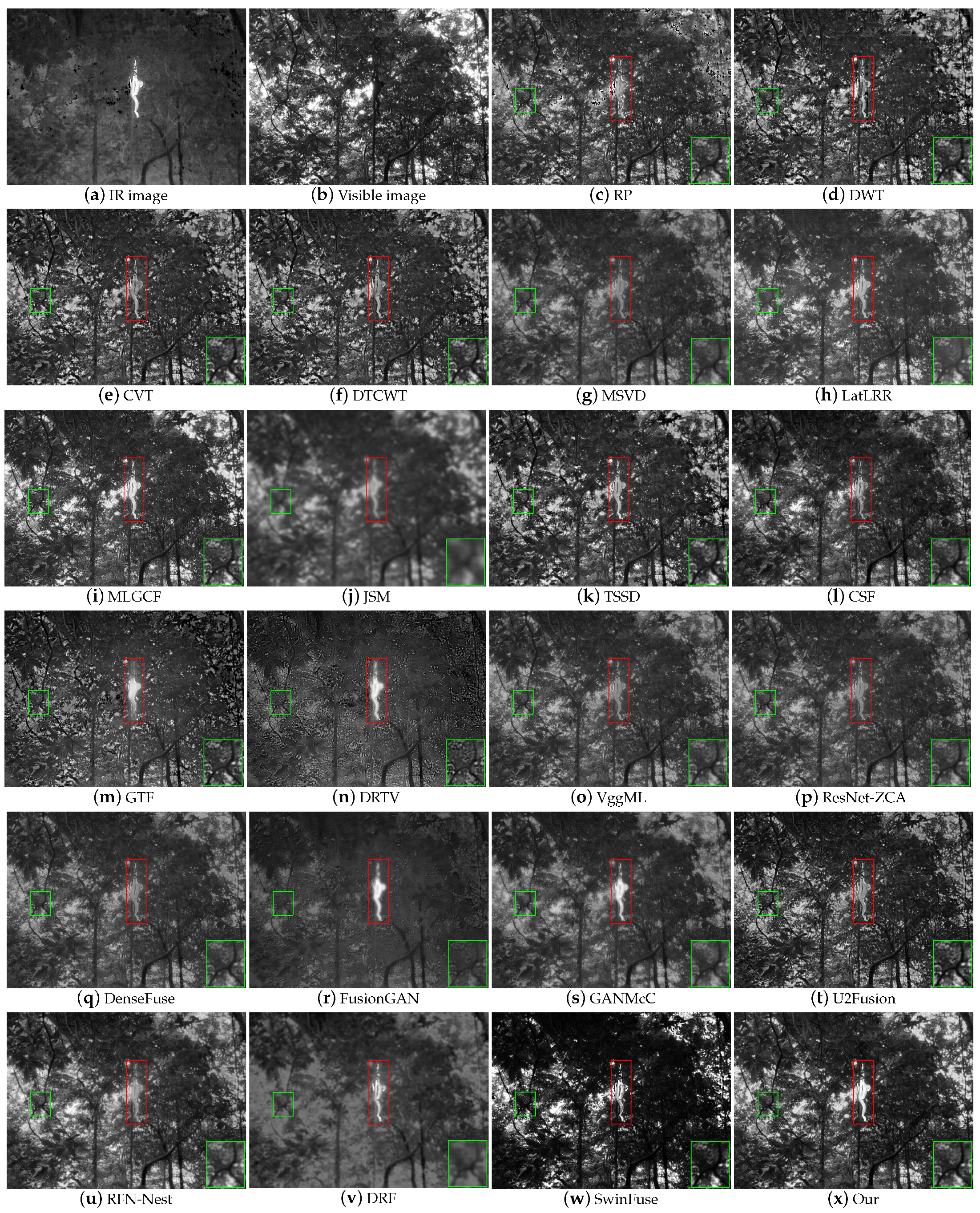
Figure 18 and Figure 19 show more examples.

Table 7. The average values of different methods on the Hainan gibbon dataset.

Method	$\mathit{EN}$	$\mathit{SD}$	${\mathit{Q}}_{\mathit{MI}}$	${\mathit{Q}}_{\mathit{NCIE}}$	${\mathit{Q}}_{\mathit{P}}$	${\mathit{Q}}_{\mathit{CV}}$	$\mathit{VIF}$	$\mathit{MI}$
RP	7.1900	41.6702	0.2714	0.8039	0.4132	718.0131	0.7074	1.9215
DWT	7.2141	44.1572	0.2673	0.8043	0.5452	331.0208	0.7170	1.9181
CVT	7.1751	42.8986	0.2623	0.8042	0.5695	311.9264	0.6900	1.8760
DTCWT	7.1651	42.8177	0.2007	0.8031	0.2887	381.1528	0.5872	1.4343
MSVD	6.8682	32.4591	0.2772	0.8038	0.3213	472.2735	0.6768	1.9276
LatLRR	7.0301	39.3770	0.3128	0.8043	0.4524	362.1853	0.6560	2.1853
MLGCF	7.1850	46.7326	0.3384	0.8053	0.5387	237.2870	0.7471	2.4118
JSM	6.7914	30.8472	0.1872	0.8027	0.0435	1107.6623	0.2369	1.2778
TSSD	7.2002	44.2699	0.2764	0.8043	0.5289	227.4334	0.7773	1.9750
CSF	7.1128	39.7546	0.2976	0.8042	0.4305	491.2285	0.6726	2.0935
GTF	6.9333	38.5621	0.2034	0.8029	0.5079	792.7470	0.6130	1.4064
DRTV	6.1445	31.4192	0.1970	0.8028	0.2247	1389.3428	0.4882	1.2674
VggML	6.8955	33.5505	0.3385	0.8049	0.5244	414.4148	0.6934	2.3531
ResNet-ZCA	6.8761	32.9442	0.3316	0.8048	0.5129	413.8779	0.6877	2.3010
DenseFuse	6.8599	32.4391	0.3406	0.8049	0.5048	437.2690	0.6803	2.3596
FusionGAN	6.2767	22.0895	0.2550	0.8034	0.1970	1435.6146	0.4683	1.6515
GANMcC	7.0135	36.1804	0.3260	0.8046	0.4395	585.5526	0.6397	2.2785
U2Fusion	7.0568	42.9271	0.2775	0.8039	0.4512	436.9586	0.6375	1.9436
RFN-Nest	7.2953	43.1552	0.2915	0.8042	0.4314	437.7463	0.7083	2.0785
DRF	6.6997	28.0482	0.2301	0.8031	0.0729	1148.9914	0.4572	1.5634
SwinFuse	6.6527	50.0185	0.3633	0.8049	0.4295	472.7369	0.6685	2.4522
Our	7.0999	46.9677	0.4393	0.8095	0.5999	194.4086	0.9018	3.1424

exhibits the average values of different objective evaluation metrics on the Hainan gibbon dataset, where the best values are indicated in red font. The proposed method achieved six best values ($Q_{MI}$, $Q_{NCIE}$, $Q_P$, $Q_{CV}$, $VIF$, $MI$) and a second-best values ($SD$).

5. Discussion

In general, the experiments on the three datasets exhibit that the proposed approach has a better fusion performance than the 21 comparison methods, which proves that the proposed approach can be applied not only in the military field (TNO dataset) and civil field (RoadScene dataset), but also in the field of observation of endangered animals (Hainan gibbon dataset). Therefore, the proposed approach has achieved state-of-the-art fusion performance and strong robustness. The loss function determines the distribution ratio of IR and visible features in the fusion result. The proposed loss function can effectively improve fusion performance. In addition, our method has a limitation: the two-stage training method is very time-consuming. Therefore, in future work, we will try to change the network to one-stage training.

6. Conclusions

In this paper, we propose an end-to-end salient detection method for infrared and visible image fusion called SDRSwin. The loss function determines the distribution ratio of IR and visible features in the fusion result. We develop a novel salient loss function to guide the network to fuse the salient targets in the infrared image and the background detail regions in the visible image. The extensive results of the TNO, RoadScene, and Hainan gibbon datasets indicate that our method has abundant texture details with clear bright infrared targets and achieves a better performance than the twenty-one state-of-the-art methods in both subjective and objective evaluation. In future work, we will apply SDRSwin to remote sensing image fusion, medical image fusion, and multi-focus image fusion.

References

1. Qi, B.; Jin, L.; Li, G.; Zhang, Y.; Li, Q.; Bi, G.; Wang, W. Infrared and Visible Image Fusion Based on Co-Occurrence Analysis Shearlet Transform. Remote Sens. 2022, 14, 283. [Google Scholar] [CrossRef]
2. Li, C.; Zhu, C.; Zhang, J.; Luo, B.; Wu, X.; Tang, J. Learning local-global multi-graph descriptors for RGB-T object tracking. IEEE Trans. Circuits Syst. Video Technol. 2018, 29, 2913–2926. [Google Scholar] [CrossRef]
3. Li, C.; Liang, X.; Lu, Y.; Zhao, N.; Tang, J. RGB-T object tracking: Benchmark and baseline. Pattern Recognit. 2019, 96, 106977. [Google Scholar] [CrossRef]
4. Luo, C.; Sun, B.; Yang, K.; Lu, T.; Yeh, W.C. Thermal infrared and visible sequences fusion tracking based on a hybrid tracking framework with adaptive weighting scheme. Infrared Phys. Technol. 2019, 99, 265–276. [Google Scholar] [CrossRef]
5. Krishnan, B.S.; Jones, L.R.; Elmore, J.A.; Samiappan, S.; Evans, K.O.; Pfeiffer, M.B.; Blackwell, B.F.; Iglay, R.B. Fusion of visible and thermal images improves automated detection and classification of animals for drone surveys. Sci. Rep. 2023, 13, 10385. [Google Scholar] [CrossRef]
6. Toet, A. Image fusion by a ratio of low-pass pyramid. Pattern Recognit. Lett. 1989, 9, 245–253. [Google Scholar] [CrossRef]
7. Li, H.; Manjunath, B.; Mitra, S.K. Multisensor image fusion using the wavelet transform. Graph. Model. Image Process. 1995, 57, 235–245. [Google Scholar] [CrossRef]
8. Nencini, F.; Garzelli, A.; Baronti, S.; Alparone, L. Remote sensing image fusion using the curvelet transform. Inf. Fusion 2007, 8, 143–156. [Google Scholar] [CrossRef]
9. Lewis, J.J.; O’Callaghan, R.J.; Nikolov, S.G.; Bull, D.R.; Canagarajah, N. Pixel-and region-based image fusion with complex wavelets. Inf. Fusion 2007, 8, 119–130. [Google Scholar] [CrossRef]
10. Naidu, V. Image fusion technique using multi-resolution singular value decomposition. Def. Sci. J. 2011, 61, 479. [Google Scholar] [CrossRef]
11. Li, H.; Wu, X.J. Infrared and visible image fusion using latent low-rank representation. arXiv 2018, arXiv:1804.08992. [Google Scholar]
12. Tan, W.; Zhou, H.; Song, J.; Li, H.; Yu, Y.; Du, J. Infrared and visible image perceptive fusion through multi-level Gaussian curvature filtering image decomposition. Appl. Opt. 2019, 58, 3064–3073. [Google Scholar] [CrossRef] [PubMed]
13. Zhang, Q.; Fu, Y.; Li, H.; Zou, J. Dictionary learning method for joint sparse representation-based image fusion. Opt. Eng. 2013, 52, 057006. [Google Scholar] [CrossRef]
14. Gao, Z.; Zhang, C. Texture clear multi-modal image fusion with joint sparsity model. Optik 2017, 130, 255–265. [Google Scholar] [CrossRef]
15. Bavirisetti, D.P.; Dhuli, R. Two-scale image fusion of visible and infrared images using saliency detection. Infrared Phys. Technol. 2016, 76, 52–64. [Google Scholar] [CrossRef]
16. Ma, J.; Zhou, Z.; Wang, B.; Zong, H. Infrared and visible image fusion based on visual saliency map and weighted least square optimization. Infrared Phys. Technol. 2017, 82, 8–17. [Google Scholar] [CrossRef]
17. Xu, H.; Zhang, H.; Ma, J. Classification saliency-based rule for visible and infrared image fusion. IEEE Trans. Comput. Imaging 2021, 7, 824–836. [Google Scholar] [CrossRef]
18. Ma, J.; Chen, C.; Li, C.; Huang, J. Infrared and visible image fusion via gradient transfer and total variation minimization. Inf. Fusion 2016, 31, 100–109. [Google Scholar] [CrossRef]
19. Du, Q.; Xu, H.; Ma, Y.; Huang, J.; Fan, F. Fusing infrared and visible images of different resolutions via total variation model. Sensors 2018, 18, 3827. [Google Scholar] [CrossRef]
20. Liang, J.; Cao, J.; Sun, G.; Zhang, K.; Van Gool, L.; Timofte, R. Swinir: Image restoration using swin transformer. In Proceedings of the IEEE/CVF International Conference on Computer Vision, Montreal, BC, Canada, 11–17 October 2021; pp. 1833–1844. [Google Scholar]
21. Wang, Z.; Chen, Y.; Shao, W.; Li, H.; Zhang, L. SwinFuse: A Residual Swin Transformer Fusion Network for Infrared and Visible Images. arXiv 2022, arXiv:2204.11436. [Google Scholar] [CrossRef]
22. Li, H.; Wu, X.J.; Kittler, J. RFN-Nest: An end-to-end residual fusion network for infrared and visible images. Inf. Fusion 2021, 73, 72–86. [Google Scholar] [CrossRef]
23. Ma, J.; Yu, W.; Liang, P.; Li, C.; Jiang, J. FusionGAN: A generative adversarial network for infrared and visible image fusion. Inf. Fusion 2019, 48, 11–26. [Google Scholar] [CrossRef]
24. Li, H.; Wu, X.J.; Kittler, J. Infrared and visible image fusion using a deep learning framework. In Proceedings of the 2018 24th International Conference on Pattern Recognition (ICPR), Beijing, China, 20–24 August 2018; pp. 2705–2710. [Google Scholar]
25. Simonyan, K.; Zisserman, A. Very deep convolutional networks for large-scale image recognition. arXiv 2014, arXiv:1409.1556. [Google Scholar]
26. Li, H.; Wu, X.J.; Durrani, T.S. Infrared and visible image fusion with ResNet and zero-phase component analysis. Infrared Phys. Technol. 2019, 102, 103039. [Google Scholar] [CrossRef]
27. Li, S.; Zou, Y.; Wang, G.; Lin, C. Infrared and Visible Image Fusion Method Based on a Principal Component Analysis Network and Image Pyramid. Remote Sens. 2023, 15, 685. [Google Scholar] [CrossRef]
28. Li, H.; Wu, X.J. DenseFuse: A fusion approach to infrared and visible images. IEEE Trans. Image Process. 2018, 28, 2614–2623. [Google Scholar] [CrossRef]
29. Xu, H.; Wang, X.; Ma, J. DRF: Disentangled representation for visible and infrared image fusion. IEEE Trans. Instrum. Meas. 2021, 70, 1–13. [Google Scholar] [CrossRef]
30. Ma, J.; Zhang, H.; Shao, Z.; Liang, P.; Xu, H. GANMcC: A generative adversarial network with multiclassification constraints for infrared and visible image fusion. IEEE Trans. Instrum. Meas. 2020, 70, 1–14. [Google Scholar] [CrossRef]
31. Xu, H.; Ma, J.; Jiang, J.; Guo, X.; Ling, H. U2Fusion: A unified unsupervised image fusion network. IEEE Trans. Pattern Anal. Mach. Intell. 2020, 44, 502–518. [Google Scholar] [CrossRef]
32. Vaswani, A.; Shazeer, N.; Parmar, N.; Uszkoreit, J.; Jones, L.; Gomez, A.N.; Kaiser, Ł.; Polosukhin, I. Attention is all you need. In Advances in Neural Information Processing Systems 30 (NIPS 2017); NeurIPS: La Jolla, CA, USA, 2017; Volume 30. [Google Scholar]
33. Dosovitskiy, A.; Beyer, L.; Kolesnikov, A.; Weissenborn, D.; Zhai, X.; Unterthiner, T.; Dehghani, M.; Minderer, M.; Heigold, G.; Gelly, S.; et al. An image is worth 16x16 words: Transformers for image recognition at scale. arXiv 2020, arXiv:2010.11929. [Google Scholar]
34. Liu, Z.; Lin, Y.; Cao, Y.; Hu, H.; Wei, Y.; Zhang, Z.; Lin, S.; Guo, B. Swin transformer: Hierarchical vision transformer using shifted windows. In Proceedings of the IEEE/CVF International Conference on Computer Vision, Montreal, BC, Canada, 11–17 October 2021; pp. 10012–10022. [Google Scholar]
35. Cao, H.; Wang, Y.; Chen, J.; Jiang, D.; Zhang, X.; Tian, Q.; Wang, M. Swin-unet: Unet-like pure transformer for medical image segmentation. In Proceedings of the European Conference on Computer Vision, Tel Aviv, Israel, 23–27 October 2022; pp. 205–218. [Google Scholar]
36. Lin, L.; Fan, H.; Xu, Y.; Ling, H. Swintrack: A simple and strong baseline for transformer tracking. arXiv 2021, arXiv:2112.00995. [Google Scholar]
37. Toet, A. TNO Image Fusion Dataset. 2014. Available online: https://figshare.com/articles/TN_Image_Fusion_Dataset/1008029 (accessed on 1 June 2023).
38. Xu, H.; Ma, J.; Le, Z.; Jiang, J.; Guo, X. Fusiondn: A unified densely connected network for image fusion. Aaai Conf. Artif. Intell. 2020, 34, 12484–12491. [Google Scholar] [CrossRef]
39. Zhang, H.; Turvey, S.T.; Pandey, S.P.; Song, X.; Sun, Z.; Wang, N. Commercial drones can provide accurate and effective monitoring of the world’s rarest primate. Remote. Sens. Ecol. Conserv. 2023. [Google Scholar] [CrossRef]
40. Wang, X.; Wen, S.; Niu, N.; Wang, G.; Long, W.; Zou, Y.; Huang, M. Automatic detection for the world’s rarest primates based on a tropical rainforest environment. Glob. Ecol. Conserv. 2022, 38, e02250. [Google Scholar] [CrossRef]
41. IUCN. The IUCN Red List of Threatened Species. Version 2019-2, 2019. Available online: http://www.iucnredlist.org (accessed on 1 June 2023).
42. Estrada, A.; Garber, P.A.; Rylands, A.B.; Roos, C.; Fernandez-Duque, E.; Di Fiore, A.; Nekaris, K.A.I.; Nijman, V.; Heymann, E.W.; Lambert, J.E.; et al. Impending extinction crisis of the world’s primates: Why primates matter. Sci. Adv. 2017, 3, e1600946. [Google Scholar] [CrossRef]
43. Zhang, H.; Wang, C.; Turvey, S.T.; Sun, Z.; Tan, Z.; Yang, Q.; Long, W.; Wu, X.; Yang, D. Thermal infrared imaging from drones can detect individuals and nocturnal behavior of the world’s rarest primate. Glob. Ecol. Conserv. 2020, 23, e01101. [Google Scholar] [CrossRef]
44. He, K.; Zhang, X.; Ren, S.; Sun, J. Deep residual learning for image recognition. In Proceedings of the IEEE Conference on Computer Vision and Pattern Recognition, Las Vegas, NV, USA, 27–30 June 2016; pp. 770–778. [Google Scholar]
45. Huang, G.; Liu, Z.; Van Der Maaten, L.; Weinberger, K.Q. Densely connected convolutional networks. In Proceedings of the IEEE Conference on Computer Vision and Pattern Recognition, Honolulu, HI, USA, 21–26 July 2017; pp. 4700–4708. [Google Scholar]
46. Wang, Z.; Bovik, A.C.; Sheikh, H.R.; Simoncelli, E.P. Image quality assessment: From error visibility to structural similarity. IEEE Trans. Image Process. 2004, 13, 600–612. [Google Scholar] [CrossRef]
47. Lin, T.Y.; Maire, M.; Belongie, S.; Hays, J.; Perona, P.; Ramanan, D.; Dollár, P.; Zitnick, C.L. Microsoft coco: Common objects in context. In Proceedings of the European Conference on Computer Vision, Zurich, Switzerland, 6–12 September 2014; pp. 740–755. [Google Scholar]
48. Hwang, S.; Park, J.; Kim, N.; Choi, Y.; So Kweon, I. Multispectral pedestrian detection: Benchmark dataset and baseline. In Proceedings of the IEEE Conference on Computer Vision and Pattern Recognition, Boston, MA, USA, 7–12 June 2015; pp. 1037–1045. [Google Scholar]
49. Roberts, J.W.; Van Aardt, J.A.; Ahmed, F.B. Assessment of image fusion procedures using entropy, image quality, and multispectral classification. J. Appl. Remote Sens. 2008, 2, 023522. [Google Scholar]
50. Rao, Y.J. In-fibre Bragg grating sensors. Meas. Sci. Technol. 1997, 8, 355. [Google Scholar] [CrossRef]
51. Hossny, M.; Nahavandi, S.; Creighton, D. Comments on ‘Information measure for performance of image fusion’. Electron. Lett. 2008, 44, 1066–1067. [Google Scholar] [CrossRef]
52. Wang, Q.; Shen, Y.; Jin, J. Performance evaluation of image fusion techniques. Image Fusion Algorithms Appl. 2008, 19, 469–492. [Google Scholar]
53. Zhao, J.; Laganiere, R.; Liu, Z. Performance assessment of combinative pixel-level image fusion based on an absolute feature measurement. Int. J. Innov. Comput. Inf. Control 2007, 3, 1433–1447. [Google Scholar]
54. Chen, H.; Varshney, P.K. A human perception inspired quality metric for image fusion based on regional information. Inf. Fusion 2007, 8, 193–207. [Google Scholar] [CrossRef]
55. Sheikh, H.R.; Bovik, A.C. Image information and visual quality. IEEE Trans. Image Process. 2006, 15, 430–444. [Google Scholar] [CrossRef] [PubMed]
56. Qu, G.; Zhang, D.; Yan, P. Information measure for performance of image fusion. Electron. Lett. 2002, 38, 1. [Google Scholar] [CrossRef]
Figure 1. A Hainan gibbon example of image fusion.
Remotesensing 15 04467 g001
Figure 2. The 4 pairs of representative examples of TNO dataset.
Remotesensing 15 04467 g002
Figure 3. The 4 pairs of representative examples of RoadScene dataset.
Remotesensing 15 04467 g003
Figure 4. The 4 pairs of representative examples of Hainan gibbon dataset.
Remotesensing 15 04467 g004
Figure 5. The fusion model proposed in this paper. The RDFN denotes the residual dense fusion network, the RSTL represents the residual Swin Transformer layer, and the Conv stands for convolutional layer.
Remotesensing 15 04467 g005
Figure 6. The structure of RSTL. The STB denotes the Swin Transformer Block.
Remotesensing 15 04467 g006
Figure 7. The architecture of two successive Swin Transformer blocks.
Remotesensing 15 04467 g007
Figure 8. The architecture of RDFN. Φ A 3 and Φ B 3 indicate the IR and visible features extracted by the encoder, respectively, and Φ F 0 denotes the fused feature.
Remotesensing 15 04467 g008
Figure 9. The training method in the first stage.
Remotesensing 15 04467 g009
Figure 10. The training model proposed in the second stage.
Remotesensing 15 04467 g010
Figure 11. Fusion results of the “Queen Road” source images.
Remotesensing 15 04467 g011
Figure 12. Fusion results of the “Kaptein1123” source images.
Remotesensing 15 04467 g012
Figure 13. Fusion results of the “Kaptein1654” source images.
Remotesensing 15 04467 g013
Figure 14. Fusion results of the “FLIR04602” source images.
Remotesensing 15 04467 g014
Figure 15. Fusion results of the “FLIR06430” source images.
Remotesensing 15 04467 g015
Figure 16. Fusion results of the “FLIR08835” source images.
Remotesensing 15 04467 g016
Figure 17. Fusion results of the first pair of source images.
Remotesensing 15 04467 g017
Figure 18. Fusion results of the second pair of source images.
Remotesensing 15 04467 g018
Figure 19. Fusion results of the third pair of source images.
Remotesensing 15 04467 g019