Abstract
The cool skin effect refers to the phenomenon where the surface skin temperature of the ocean is always slightly cooler than the temperature of the water directly underneath due to the ubiquitous cooling processes at the ocean surface, especially in the absence of solar radiation. The cool skin effect plays a critical role in the estimation of heat, momentum, and gas exchange between the air and the sea. However, the scarcity of observational data greatly hinders the accurate assessment of the cool skin effect. Here, the matchup data from the new generation geostationary satellite Himawari-8 and in situ sea surface temperature (SST) observations are used to evaluate the performance and dependence on the cool skin effect in the low/mid-latitude oceans. Results show that the intensity of the cool skin effect as revealed by Himawari-8 (−0.16 K) is found to be relatively weaker than previously published cool skin models based on in situ concurrent observations. A considerable amount of warm skin signals has been detected in the high-latitude oceans (e.g., Southern Ocean) under the circumstances of positive air–sea temperature difference and high wind, which may be the main cause of discrepancies with previous thoughts on the cool skin effect.
1. Introduction
Sea surface temperature (SST) acting as both an Essential Climate Variable (ECV) and an Essential Ocean Variable (EOV), plays a vital role in the climate system [1,2]. SST significantly affects the exchange of energy, momentum, and gases between the ocean and atmosphere, and thus serves as an important input in ocean models, numerical weather prediction (NWP), and climate simulations [3,4]. The definition of different SSTs is introduced by the Group for High-Resolution Sea Surface Temperature (GHRSST), based on the thermal characteristics and observing methods of the surface ocean [5]. Operationally, the skin SST (Tskin) is the temperature measured by an infrared radiometer usually mounted on a satellite or a research vessel, which shows the thermal features within the conductive diffusion-dominated sub-layer with a depth of approximately 10 to 20 μm. The temperature acquired beneath the thermal boundary layer is considered the subsurface SST, Tdepth (traditionally referred to as the bulk SST, Tbulk), which is measured at depths ranging from 10−2 to 101 m using various platforms and sensors, such as buoys, drifters, ships, and profilers.
Two key physical processes determine the surface temperature vertical gradient, i.e., the warm layer effect and the cool skin effect [6]. During the daytime, the upper ocean within a few meters of the surface is significantly warmer (typically ~3 K) than the underlying water because of the absorption of solar radiation, which is referred to as the warm layer effect. The warm layer is modulated by the intensity of local solar radiation and eliminated by turbulent mixing at night [7,8,9]. In contrast, the Tskin is always cooler than the temperature immediately below an amplitude of several tenths of Kelvin in the absence of solar radiation, which is referred to as the cool skin effect. The cool skin effect persists throughout the day due to ubiquitous heat loss occurring in the upper few millimeters of the ocean’s surface. This heat loss is caused by a combination of upward longwave radiation, latent heat flux (LHF), and sensible heat flux (SHF). However, the cool skin effect is typically counteracted by the warm layer effect during the day, as the amplitude of the cool skin effect is generally one order smaller than that of the warm layer effect.
The cool skin effect has long been recognized and parameterized into theoretical and empirical models, indicating that it is mainly modulated by variables associated with surface cooling [6,10,11,12]. Most studies have employed ship-based radiometers to obtain Tskin, ensuring high accuracy and concurrence with in situ Tdepth observations [13,14,15,16,17], and polar-orbiting satellite remote-sensed Tskin products have also been utilized to get global coverage of the cool skin effect [18]. Based on observational approaches and modeling studies, the cool skin effect has been employed in improving the accuracy of satellite SST retrieval algorithms, coupled model simulations, weather/climate predictions, and air–sea fluxes of heat and gases [19,20,21,22,23]. Especially, due to the high sensitivity of air–sea CO2 fluxes to SST [24,25], the global ocean CO2 uptake would substantially increase by ~35% to 50% considering the cool skin effect [26,27], which could greatly influence the estimation of the carbon cycle process of the earth system.
However, several factors could significantly hinder our comprehensive understanding of the cool skin effect, largely due to insufficient in situ observational data. Studies based on research cruises have shown significant seasonal and regional dependencies since remote oceans and high-sea states are not accessible for ships. Although polar-orbiting remote sensing provides global coverage and fills most of the observational gaps, the time interval of several days for a repeated cycle makes it challenging to capture continuous variability in the cool skin effect.
The development of geostationary satellites and corresponding mounted instruments has greatly enhanced our ability to obtain high-quality global SST data with high temporal–spatial resolution. The geostationary satellites are positioned over a fixed point on the equator, allowing for continuous observations of the same region with high temporal resolution. This is particularly important for understanding the mechanisms driving this phenomenon.
Himawari-8, Japan’s new generation geostationary satellite, was launched in 2014 and remained operational since 2015, equipping the state-of-the-art Advanced Himawari Imager (AHI) with outstanding spatial (from 2 km at nadir to 12 km at satellite view zenith angle ~67°), temporal (up to 10 min), spectral and radiometric resolution [28,29,30].
Himawari-8 is positioned over the equatorial western Pacific, which encompasses the mid-to-low latitude oceans of the western Pacific, the eastern Indian Ocean, and a portion of the Southern Ocean. Additionally, Himawari-8’s coverage spans a vast expanse of ocean from the equator to high latitudes, encompassing a rich variety of multiscale ocean-atmosphere processes, including mesoscale eddies and storms. This is beneficial for investigating the mechanisms and variability of the cool skin effect.
In this study, we utilize the high temporal–spatial resolution of Tskin data from geostationary satellite Himawari-8, combined with the commonly used Tdepth data from the NOAA in situ SST Quality Monitor (iQuam), to address two main issues: (1) the effectiveness of new generation geostationary satellite in detecting the cool skin effect, and (2) the dependencies of the observed cool skin effect on ocean surface wind and thermal condition. The structure of this paper is as follows. Section 2 introduces the datasets used in this study, as well as methods of data matchup and calculation of the cool skin effect. Section 3 shows the performance and dependence of the observed cool skin effect revealed by geostationary satellites. Section 4 summarizes the findings of this study and addresses some discussions.
2. Materials and Methods
2.1. Datasets
The AHI SST products are generated by the NOAA’s Advanced Clear-Sky Processor for Oceans (ACSPO) system and distributed by GHRSST following the recommended GHRSST Data Specification (GDS) version 2 [31,32]. The ACSPO AHI SST data are derived using the ACSPO Clear-Sky Mask (ACSM) and Non-Linear SST (NLSST) algorithm utilizing 4 AHI bands centered at 8.6, 10.4, 11.2, and 12.4 µm [33]. Here, SST data with a temporal–spatial resolution of hourly and 0.02° are used from level 3 collected (L3C), version 2.71 Himawari-8 AHI dataset from January 2020 to December 2022, which cover widely ranged oceans in the low/mid-latitudes (Figure 1). The SST data of AHI are obtained from retrieval algorithms trained against the night-time analysis L4 SST, while the sensitivity to the real skin temperature is quite high; thus, the AHI SST product could be considered a great estimate of Tskin [30,34,35]. Only data of the highest quality (quality level, QL = 5) are used in the study.
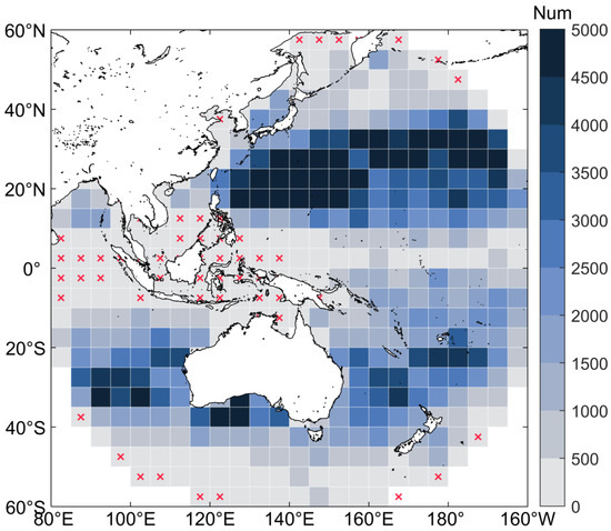
Figure 1.
Count of matchup data within each 5° by 5° box. The cross marks denote less than 100 data pairs in the box.
The in situ SST data are accessed from iQuam developed by NOAA National Environmental Satellite Data and Information Services/Centre for Satellite Applications and Research (STAR). The iQuam SST data are obtained by a variety of different observation platforms (drifter, ship, buoy, Argo float, etc.) sharing uniform quality control algorithms [36]. Considering the vast number of available data, as well as the uniform design and configuration, SST data obtained only by drifting buoys (observed at depth ~0.2 m) are introduced as the Tdepth (while Tdepth data from other platforms have also been examined and no significant impact of the observational platform on the conclusions was found, which is not shown in this paper). Similarly, only in situ SST data with the highest quality (QL = 5) are used for further calculation.
Environmental variables of the air–sea interface from the European Centre for Medium-Range Weather Forecasts (ECMWF) reanalysis products are included to estimate the performance and implication of the cool skin effect. Hourly 10 m wind (U10), SHF, LHF, shortwave radiation (SWR), and net longwave radiation (LWR) data provided by ReAnalysis 5th Generation (ERA5) are used for evaluation of the dependence of the cool skin effect. We also use the monthly sea surface salinity (SSS) and sea ice fraction (SIF) data of Ocean ReAnalysis System 5 (ORAS5) for the calculation of the air–sea CO2 flux. Those reanalysis data have a spatial resolution of 0.25°. Furthermore, the monthly global surface air and ocean pCO2 product at 1° 1° are used in the calculation of ocean CO2 storage [37].
2.2. Data Matchup
The remote-sensed Tskin and in situ Tdepth are matched up under the temporal and spatial window of 30 min and 0.02°, which provides more massive and high-resolution matchup data owing to the benefits of new-generation geostationary satellites. Only night-time data pairs are used in order to remove the warm layer effect. Here, apparent sunrise/sunset, rather than physical sunrise/sunset, is used to separate day and night, where the apparent sunrise/sunset time will be slightly earlier/later than the physical sunrise/sunset time due to atmospheric refraction. This is achieved by a local sunrise/sunset time algorithm with correction for the approximate effects of atmospheric refraction [38]. In this study, the night-time is more strictly defined as the period between 1 h after apparent sunset and apparent sunrise. It is worth noting that setting a 1 h delay in the sunset time could significantly reduce the average shortwave radiation from 1.633 W/m2 to 0.031 W/m2 as compared to no delay in sunset time. This reduction in shortwave radiation could effectively eliminate the lag effect of the warm layer effect [7]. Additionally, the ERA5 wind data are collocated with SST matchups by a 2D fitting strategy of the nearest neighbor.
The matchup data include a total number of 656,213 collocations (Figure 1). It is important to mention that the distribution of the matched data exhibits significant regional nonuniformity, which can be attributed to the deployment interests and strategies of in situ observation implementers. Specifically, some regions such as the tropical oceans, high latitudes, and marginal seas (e.g., the South China Sea) have a sparser distribution of in situ observations as compared to mid-latitude oceans. Therefore, the results from the matched data will inevitably be biased towards the mid-latitude regions.
Since the solar absorption and its lag effect are removed by adopting the night-time SST matchups, the cool skin effect could be simply derived by the difference between skin SST and depth SST, i.e.,
ΔT = Tskin − Tdepth
Note that some studies have defined the ΔT as the difference between Tdepth and Tskin and their findings exhibit an opposite sign in comparison to this study.
3. Results
3.1. Cool Skin Effect as Seen from Himawari-8 SST
The majority of regions within the Himawari-8 domain exhibit a surface cooling pattern (Figure 2), except for boxes at high latitudes or with few data pairs (marked with crosses). It is worth noting that a significant number of warm skin signals have been observed in the Sea of Okhotsk and the Southern Ocean. In the low/mid-latitude oceans, the Himawari-8 and iQuam matchup data are sufficient to reveal the cool skin effect, which is consistent with previous findings. The high-latitude scenario will be discussed in a subsequent chapter.
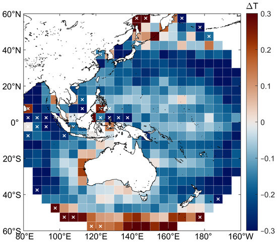
Figure 2.
Mean ΔT of matchup data within each 5° by 5° box. The cross marks denote less than 100 data pairs in the box.
The satellite view zenith angle (VZA) is an important factor that may influence the performance of geostationary satellite SST observations. The VZA affects the scan spatial resolution, geometric distortion, atmospheric path length, and signal-to-noise ratio of satellite images, which is critical for data retrieval and quality control algorithms of geostationary satellites. It has been reported that there is a significant drift of skin temperature with VZA for the Himawari-8 product of the Japan Aerospace Exploration Agency (JAXA), indicating the ΔT values are much larger under a larger VZA [39].
Here, the dependence of ΔT on VZA was examined and shown in Figure 3. The majority of the ΔT matchup data fall in the range of VZA over 20 degrees, while the data for the nadir are rather poor. Overall, the ΔT is relatively stable throughout the coverage of Himawari-8 but shows a slight trend with increasing VZA. This suggests slightly colder skin at the edge of the Himawari-8 disk, but the phenomenon is not exactly centrosymmetric. For instance, the high-latitude oceans exhibit much warmer skin temperatures, although they share the same larger VZA as the tropical oceans near 160°W. Therefore, although ΔT shows slight dependence on VZA, the spatial variabilities within the Himawari-8 domain still need to be further discussed.
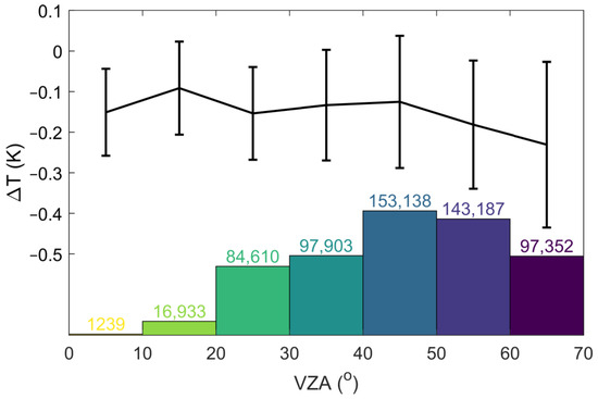
Figure 3.
The dependence of ΔT on VZA, error bars denote the half standard deviation, column bars denote matchup counts in every 10 deg VZA interval.
Histograms and basic statistics of the cool skin effect are shown in Figure 4. A quasi-Gaussian distribution of the ΔT is found with a mean value of −0.16 K. Note that the mean amplitude of ΔT as revealed by the geostationary satellite is slightly weaker than previous cool skin models [13,15,16,17], with a typical value of −0.17 K reported by [14].
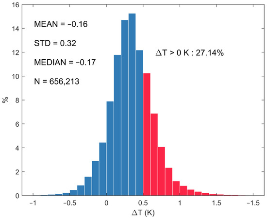
Figure 4.
Histograms and basic statistics of the matchup ΔT.
An inter-model comparison reveals distinct differences among observation methods, as shown in Table 1. In situ observational studies, which rely on ship or buoy data, reported a much larger cool skin amplitude, albeit with a limited number of matchup data. Nevertheless, the estimations based on remote sensing, utilizing either polar-orbiting or geostationary satellites, exhibit a large volume of data and standard deviations (STD), which consistently demonstrate small amplitudes of the cool skin effect [18].

Table 1.
Basic information and statistics of different cool skin models.
The large STDs that are derived from satellite remote sensing data might be attributed to the large matchup window. In terms of spatial distribution, the lack of concurrent observations may introduce biases arising from small-scale variability. However, the temporal matchup windows related to remote sensing and in situ observations (30 min to 1 h) are longer than in situ concurrent observations (usually a few seconds) due to the temporal resolution limitations of the satellite Tskin products.
Another issue worth noting is the existence of a “warm skin” phenomenon, where ΔT > 0 K. By the definition of the cool skin effect mentioned above, the night-time Tskin is always colder than Tdepth due to several surface cooling mechanisms. However, the present study reveals that 27.1% of the observed ΔT values are greater than zero, indicating the presence of a warmer skin. This phenomenon has also been observed by R/V and polar-orbiting remote sensing, but with a smaller proportion [18]. Apart from the potential impacts of data noise on the results, the positive ΔT values may be attributed to two factors, i.e., the residual solar radiation and warmer skin caused by surface ocean heating. As mentioned in the Methods section, the residual effect of solar radiation is effectively canceled by a 1 h delay from apparent sunset. Further analysis shows that 99.68% of the selected night-time shortwave radiation is lower than 1 W/m2 for Himawari-8. In this sense, it can be concluded that the ΔT values are not due to residual solar radiation. More details about the relationship between ΔT and ocean surface heating will be discussed in a subsequent section.
3.2. Cool Skin Dependence on Wind Speed
It has been long acknowledged that the ΔT is highly sensitive to surface wind speed. The wind speed modulates the cool skin effect through two mechanisms that play the opposite effects. On the one hand, wind speed, acting as an important driver of surface heat loss, could increase ΔT by enhancing upward surface sensible and latent heat flux. On the other hand, wind speed is also an essential factor in surface turbulent mixing, which indicates that wind blowing can efficiently dampen the cool skin effect by weakening the surface stratification. Under the joint effect of the above two mechanisms, the wind exerts a dampening effect on the cool skin effect. That is, as the wind speed increases, the Tskin and Tdepth tend to converge and result in a decrease in the amplitude of ΔT.
Previous studies proposed empirical exponential functions to illustrate the effect of wind speed on the cool skin effect by least-squares fitting of the concurrent shipboard observations of Tskin and Tdepth data (Figure 5). All empirical models exhibit a similar pattern, with only slight differences in certain coefficients. ΔT is generally larger under calm winds (e.g., U10 < 5 m/s), and drops rapidly as wind speed increases. After reaching a certain speed of the wind (typically U10 ~ 6 to 8 m/s), the ΔT tends to stabilize at an asymptotic value, ranging from −0.13 K to −0.30 K in previously published results.
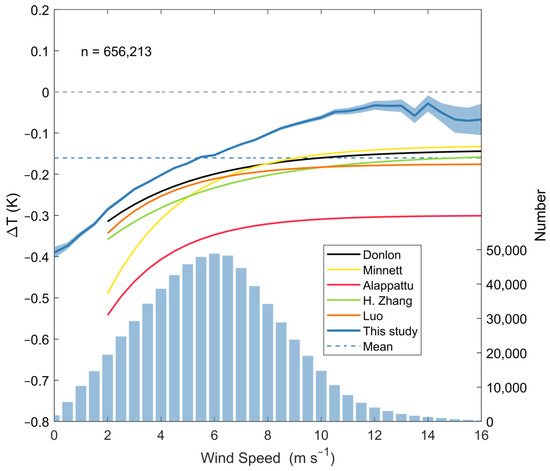
Figure 5.
Cool skin dependence on wind speed. The blue solid line denotes the mean ΔT within every 0.5 m/s wind speed interval. The blue shading denotes the 95% confidence level margin of error (1.96 times the STD divided by the square root of the collocation number). The gray and blue dashed lines represent the ΔT = 0 and the average ΔT in this study, respectively. The blue column bars denote the matchup counts within every 0.5 m/s wind speed interval. The solid lines of black, yellow, red, green, and orange represent cool skin models from [13,14,15,16,17], respectively.
The relationship between the cool skin effect and wind speed, as revealed by Himawari-8 and in situ Tdepth, is presented in Figure 5. Overall, our findings show a similar pattern to previous studies using concurrent in situ observations, but notable discrepancies remain clear. ΔT decreases monotonically with increasing wind speed, and the overall ΔT is smaller than previous results. However, remarkable differences are observed under high winds. The asymptotic ΔT value showed by Himawari-8, which tends to reach zero, is much smaller compared with in situ observation-based results. The transition point occurs at higher wind (U10 ~10 m/s) than previous results (U10 ~6–8 m/s). The relationship between ΔT and wind speed shows fewer characteristics of the exponential function, so the mean value of ΔT variation with wind speed is used for later quantification of the cool skin effect, rather than the exponential function by least-squares fitting. Notably, the cool skin effect demonstrated by geostationary satellites shares more similarities with a previous study based on polar-orbiting satellite remote sensing, as compared to results revealed by in situ observations. The overall ΔT values of both geostationary and polar-orbiting satellites (see Figure 3 of [18]) are smaller than the in situ results.
Overall, the cool skin effect exhibited by Himawari-8 appears to be weaker compared to previous studies, as indicated by statistical characteristics and the ΔT-wind pattern. Next, we will elucidate this distinction from the perspective of warm skin signals.
3.3. Warm Skin Signals
Firstly, we will explore the source of the observed warm skin signals. While wind acts as an amplifier in turbulent heat fluxes, latent heat flux typically plays a role in cooling the ocean. Hence, in order to identify the source of the warming, we will examine the relationship between the warm skin signals and the air–sea temperature difference (ΔTa-s), which influences the thermodynamic stability of the surface ocean and determines the direction of the air–sea sensible heat flux.
Figure 6 shows a significant correlation between the observed warm skin signals and ΔTa-s. The majority of ΔTa-s values are negative, corresponding to negative ΔT values. This is consistent with the expected scenario of night-time surface ocean cooling. However, about 10% of ΔTa-s values are still positive, corresponding to the cold ocean under warm air. When ΔTa-s is greater than zero, ΔT also increases to positive values, indicating a warm skin.
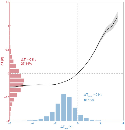
Figure 6.
Cool skin dependence on the air–sea temperature difference. The black solid line denotes the mean ΔT within every 0.5 K ΔTa-s interval. The gray shading denotes the 95% confidence level margin of error. The blue and red bars denote the histograms of ΔTa-s and ΔT, respectively.
The ΔTa-s determines the direction of air–sea sensible heat transport. The primary source of the warm skin signal is likely the air–sea temperature difference, which is manifested as the high correlation between ΔT and ΔTa-s. This is further supported by the relationship between the air–sea heat fluxes and ΔT, where a significant portion of the SHF is positive (13.5%), while a much smaller percentage of downward LHF was found (1.2%).
When we examine the whole domain of Himawari-8, the warm skin signals exhibit strong spatial variability (Figure 7a). Apart from pixels around the western coast of Australia, the warm skin signals are more concentrated in high-latitude oceans, with the Southern Ocean being the most representative. In the areas south of 50°S, warm skin signals are predominant in almost all boxes. The spatial distribution of warm skin signals also aligns with the distribution of positive ΔTa-s (Figure 7b) and strong winds (Figure 7c). In the case of warm skin conditions, the wind speed is also comparatively higher than that in the cold skin scenario (Figure 7d).
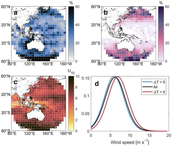
Figure 7.
(a) The percentage of positive ΔT values out of all matchup data within each 5° by 5° box. (b) The percentage of positive ΔTa-s values out of all matchup data within each 5° by 5° box. (c) Mean U10 of matchup data within each 5° by 5° box. (d) Probability density of U10 in different ΔT regimes.
In a word, warm skin signals are more prevalent in high-latitude oceans characterized by positive sea–air temperature differences and high wind speeds. These features collectively highlight the Southern Ocean region, which is rarely sampled by in situ observations. Previous studies predominantly focus on the mid-to-low latitude oceans (see Table 1). High-latitude areas with severe sea conditions pose significant challenges for ship-based observations. Furthermore, previous cool skin models mostly considered wind speeds within the range of 2 to 15 m/s, and some studies even restricted the maximum wind speed to around 10 m/s. This is due to the relatively limited number of samples from in situ observations under high wind speeds. In this study, the advantage of a large sample size obtained by Himawari-8 facilitates a more representative dataset for high-latitude and high-wind-speed conditions, revealing more warm skin signals and a weaker cool skin effect.
Limited to the absence of concurrent observational data, a statistical analysis is used to examine warm skin signals instead of conducting case studies on individual processes. Overall, the observed warm skin signals are strongly related to the air–sea temperature difference. However, there are two aspects that should be noted. Firstly, the proportion of positive air–sea temperature differences (10.15%) and downward sensible heat fluxes (13.49%) are lower than that of warm skin signals (27.14%), suggesting that while sensible heat heating may be the primary cause of warm skin signals, but not the only one. Secondly, only downward sensible heat fluxes are observed rather than the net heat fluxes. This indicates that the real surface heating phenomenon is probably not accurately represented in the reanalyzed data. Nevertheless, it confirms the significant potential of sensible heat heating in the warm surface layer. To further explore the nature and mechanism of warm skin signals, more ocean–atmosphere in situ concurrent observations are critically required, especially in the high-latitude oceans.
4. Discussion
Benefiting from the high spatial and temporal resolution of the new generation of geostationary satellite observations, an abundant amount of skin temperature and bulk temperature matchup data are used to support new explorations of the cool skin effect. Here, we show that skin temperature provided by AHI equipped on Himawari-8 effectively reveals the cool skin effect, indicating the ability of geostationary satellite observations to deal with issues such as the sensitivity of satellite retrieval SST to skin temperature and spatial dependence of remote sensing performance.
This paper shows new observation-based evidence for the cool skin effect using a vast sample of satellite remote sensing skin temperature data. A weaker cool skin effect is observed in the full disk of the Himawari-8 domain compared with previously published results from in situ skin temperature observations and satellite remote sensing. The main cause of this discrepancy may be attributed to the warm skin signals observed in the high-latitude oceans (e.g., Southern Ocean) under the circumstances of positive air–sea temperature difference and high winds. Once the wind speed exceeds 10 m/s, the cool skin seems to be efficiently eliminated.
The highlight of this study is the large number of warm skin signals detected in high latitudes compared to previous in situ observation-based studies. We believe that this phenomenon represents the real air–sea sensible heat exchange scenario, but still needs to be confirmed by in situ observations, especially in the high-latitude oceans with strong winds. Another issue with geostationary satellites is the need to improve data quality at the edge of the disk, which can be achieved by optimizing atmospheric correction in satellite data retrieval algorithms.
Although the cool skin effect has been extensively addressed in different observational studies, its accuracy is still far from adequate in model parameterization as well as in the calculation of gas fluxes. Particularly, the calculation of CO2 fluxes is extremely sensitive to the surface temperature, where the inter-model bias is considerable. The larger CO2 uptake induced by a cooler surface ranges from 0.35 PgC/year to 0.9 PgC/year in previously published results [26,27], which is considered to be rather large compared to the climatology ocean CO2 sink (2.0 PgC/year in 2000, from results from [25]). In this study, the cool skin effect associated with wind speed is carried out in global oceanic CO2 uptake (Method see Appendix A). Results show that the ocean carbon intake increases by ~0.2 pgC/year under the cool skin correction related to Himawari-8, which is significantly weaker than previous findings (Figure 8). Particularly, as the main carbon sink in the global climate system, the Southern Ocean shows more uncertainty in the cool skin effect among different studies. It can be argued that the temperature correction for CO2 fluxes is still far from operational, as a full understanding of the spatial and temporal characteristics and the mechanisms of the cool skin effect is demanded with urgency.
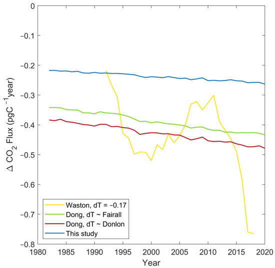
Figure 8.
Enhancement of air–sea CO2 flux (upward positive) due to different cool skin corrections. The yellow line represents the cool skin corrected CO2 flux reported by [26] which considering a constant cool skin effect (ΔT = −0.17 K). The green and red lines denote the cool skin corrected CO2 flux reported by [27] considering cool skin model of [6,14], respectively.
More actions are critically needed for a better understanding of the cool skin effect, and more observational data from high-latitude oceans may help us achieve them. Concurrent integrated high-resolution in situ observations are still necessary as the baseline for the cool skin pattern, as most of the ocean surface sub-layers have not been observed. Furthermore, the satellite retrieval algorithms could be further improved to enhance the representativeness of the retrieved SST to the real skin temperature. Accurate estimates of ocean carbon uptake require a more robust cool skin model that is suitable for the global ocean.
Author Contributions
Conceptualization, Y.Z. and Z.C.; methodology, Y.Z.; software, Y.Z.; validation, Y.Z.; formal analysis, Y.Z.; investigation, Y.Z.; resources, Y.Z.; data curation, Y.Z.; writing—original draft preparation, Y.Z.; writing—review and editing, Y.Z. and Z.C.; visualization, Y.Z.; supervision, Z.C.; project administration, Z.C.; funding acquisition, Z.C. All authors have read and agreed to the published version of the manuscript.
Funding
This research was financially supported by the National Natural Science Foundation of China (NSFC) (grant no. 42225601 and 42076009), Fundamental Research Funds for the Central Universities (grant no. 202072001 and 202241006). Z.C. is partly supported by the Taishan Scholar Funds (grant no. tsqn201812022).
Data Availability Statement
Himawari-8 SST data [40] are available at https://search.earthdata.nasa.gov/search/granules?portal=podaac-cloud&p=C2036877660-POCLOUD (accessed on 16 March 2023). The iQuam SST data [36] are available at https://www.star.nesdis.noaa.gov/socd/sst/iquam/data.html (accessed on 16 March 2023). ERA5 hourly data [41] are available at https://cds.climate.copernicus.eu/cdsapp#!/dataset/reanalysis-era5-single-levels?tab=form (accessed on 16 March 2023). ORAS monthly data are available at https://cds.climate.copernicus.eu/cdsapp#!/dataset/reanalysis-oras5?tab=form (accessed on 16 March 2023). The air and surface sea CO2 partial pressure data [42] are available at https://www.ncei.noaa.gov/data/oceans/ncei/ocads/data/0160558/MPI_SOM-FFN_v2021/ (accessed on 31 December 2022). The cool skin corrected air–sea CO2 flux data are available in [26,27].
Acknowledgments
We appreciate Yuanxu Dong for providing the cool skin-corrected CO2 flux data and insightful suggestions. We would like to express our gratitude to Honghai Zhang for the kind guidance on the CO2 flux calculation.
Conflicts of Interest
The authors declare no conflict of interest.
Abbreviations
The following abbreviations are used in this manuscript:
| ACSPO | Advanced Clear-Sky Processor for Oceans |
| ACSM | ACSPO Clear-Sky Mask |
| AHI | Advanced Himawari Imager |
| ECMWF | European Centre for Medium-Range Weather Forecasts |
| ECV | Essential Climate Variable |
| EOV | Essential Ocean Variable |
| ERA5 | ReAnalysis 5th Generation |
| GDS | GHRSST Data Specification |
| GHRSST | Group for High Resolution Sea Surface Temperature |
| iQuam | in situ SST Quality Monitor |
| JAXA | Japan Aerospace Exploration Agency |
| L3C | Level 3 Collected |
| LHF | Latent Heat Flux |
| LWR | Longwave Radiation |
| NLSST | Non-Linear SST |
| NWP | Numerical Weather Prediction |
| ORAS5 | Ocean ReAnalysis System 5 |
| QL | Quality Level |
| SHF | Sensible Heat Flux |
| SIF | Sea Ice Fraction |
| SSS | Sea Surface Salinity |
| SST | Sea Surface Temperature |
| STAR | Centre for Satellite Applications and Research |
| STD | Standard Deviation |
| SWR | Shortwave Radiation |
| Tbulk | Bulk SST |
| Tdepth | Subsurface SST |
| Tskin | Skin SST |
| U10 | 10 m Wind Speed |
| VZA | View Zenith Angle |
| ΔTa-s | Air–sea Temperature Difference |
Appendix A
The CO2 exchange across the air–sea interface could be described by a bulk flux equation as follows:
here, F (here in mol m−2 month−1) is the air–sea CO2 flux (upward positive as a following convention). k (in cm h−1) is the gas transfer velocity of CO2 described as the function of Schmidt number of CO2 in the seawater (Sc) and U10, adopting parameter configuration reported in [43]. K0 (in mol L−1 atm−1) is the aqueous-phase solubility of CO2 in the seawater related to SST and SSS [44]. pCO2w and pCO2a (in μatm) are the partial pressure of CO2 in water and air, respectively.
F = k × K0 (pCO2w − pCO2a)
The calculation of air–sea CO2 flux is highly sensitive to SST, and the modulation of CO2 flux by the cool skin effect can be understood in the following aspects. Firstly, Sc and K0 are functional of SST, which would change instantaneously by virtue of subtle changes in SST considering the cool skin correction. Moreover, pCO2w also significantly correlated with changes in SST. According to Henry’s law [45], the total free CO2 dissolved in seawater is the product of the solubility and the partial pressure of carbon dioxide. The equilibrium time of dissolved free CO2 in seawater is rather long, taking close to a year in the case of molecular diffusion equilibration alone. In contrast to other instantaneously changing parameters (e.g., solubility, Schmidt number, and the gas transfer velocity), the free dissolved CO2 can be considered to remain constant with the change in seawater temperature due to the cool skin correction [46,47]. Therefore, the dependence of pCO2w on temperature can be quantified as the quotient of free dissolved carbon dioxide versus solubility, where free dissolved carbon dioxide is a constant and solubility changes with cool skin correction.
Hence, the total CO2 uptake in the global ocean can be derived from the global integration of air–sea CO2 flux. In order to eliminate the error caused by the coverage of sea ice, the calculated CO2 fluxes are modified by the ice-free factor (i.e., 1 − SIF).
References
- Bojinski, S.; Verstraete, M.; Peterson, T.C.; Richter, C.; Simmons, A.; Zemp, M. The Concept of Essential Climate Variables in Support of Climate Research, Applications, and Policy. Bull. Am. Meteorol. Soc. 2014, 95, 1431–1443. [Google Scholar] [CrossRef]
- Centurioni, L.R.; Turton, J.; Lumpkin, R.; Braasch, L.; Brassington, G.; Chao, Y.; Charpentier, E.; Chen, Z.; Corlett, G.; Dohan, K.; et al. Global in situ Observations of Essential Climate and Ocean Variables at the Air–Sea Interface. Front. Mar. Sci. 2019, 6, 00419. [Google Scholar] [CrossRef]
- O’Carroll, A.G.; Armstrong, E.M.; Beggs, H.M.; Bouali, M.; Casey, K.S.; Corlett, G.K.; Dash, P.; Donlon, C.J.; Gentemann, C.L.; Høyer, J.L.; et al. Observational Needs of Sea Surface Temperature. Front. Mar. Sci. 2019, 6, 00420. [Google Scholar] [CrossRef]
- von Schuckmann, K.; Palmer, M.D.; Trenberth, K.E.; Cazenave, A.; Chambers, D.; Champollion, N.; Hansen, J.; Josey, S.A.; Loeb, N.; Mathieu, P.P.; et al. An imperative to monitor Earth’s energy imbalance. Nat. Clim. Chang. 2016, 6, 138–144. [Google Scholar] [CrossRef]
- Minnett, P.J.; Alvera-Azcárate, A.; Chin, T.M.; Corlett, G.K.; Gentemann, C.L.; Karagali, I.; Li, X.; Marsouin, A.; Marullo, S.; Maturi, E.; et al. Half a century of satellite remote sensing of sea-surface temperature. Remote Sens. Environ. 2019, 233, 111366. [Google Scholar] [CrossRef]
- Fairall, C.W.; Bradley, E.F.; Godfrey, J.S.; Wick, G.A.; Edson, J.B.; Young, G.S. Cool-skin and warm-layer effects on sea surface temperature. J. Geophys. Res. Ocean. 1996, 101, 1295–1308. [Google Scholar] [CrossRef]
- Hughes, K.G.; Moum, J.N.; Shroyer, E.L. Heat Transport through Diurnal Warm Layers. J. Phys. Oceanogr. 2020, 50, 2885–2905. [Google Scholar] [CrossRef]
- Prytherch, J.; Farrar, J.T.; Weller, R.A. Moored surface buoy observations of the diurnal warm layer. J. Geophys. Res. Ocean. 2013, 118, 4553–4569. [Google Scholar] [CrossRef]
- Thompson, E.J.; Moum, J.N.; Fairall, C.W.; Rutledge, S.A. Wind Limits on Rain Layers and Diurnal Warm Layers. J. Geophys. Res. Ocean. 2019, 124, 897–924. [Google Scholar] [CrossRef]
- Saunders, P.M. The Temperature at the Ocean-Air Interface. J. Atmos. Sci. 1967, 24, 269–273. [Google Scholar] [CrossRef]
- Hasse, L. The sea surface temperature deviation and the heat flow at the sea-air interface. Bound. Layer Meteorol. 1971, 1, 368–379. [Google Scholar] [CrossRef]
- Schluessel, P.; Emery, W.J.; Grassl, H.; Mammen, T. On the bulk-skin temperature difference and its impact on satellite remote sensing of sea surface temperature. J. Geophys. Res. Ocean. 1990, 95, 13341–13356. [Google Scholar] [CrossRef]
- Alappattu, D.P.; Wang, Q.; Yamaguchi, R.; Lind, R.J.; Reynolds, M.; Christman, A.J. Warm layer and cool skin corrections for bulk water temperature measurements for air-sea interaction studies. J. Geophys. Res. Ocean. 2017, 122, 6470–6481. [Google Scholar] [CrossRef]
- Donlon, C.J.; Minnett, P.J.; Gentemann, C.; Nightingale, T.J.; Barton, I.J.; Ward, B.; Murray, M.J. Toward Improved Validation of Satellite Sea Surface Skin Temperature Measurements for Climate Research. J. Clim. 2002, 15, 353–369. [Google Scholar] [CrossRef]
- Luo, B.; Minnett, P.J.; Szczodrak, M.; Akella, S. Regional and Seasonal Variability of the Oceanic Thermal Skin Effect. J. Geophys. Res. Ocean. 2022, 127, e2022JC018465. [Google Scholar] [CrossRef]
- Minnett, P.J.; Smith, M.; Ward, B. Measurements of the oceanic thermal skin effect. Deep Sea Res. Part II Top. Stud. Oceanogr. 2011, 58, 861–868. [Google Scholar] [CrossRef]
- Zhang, H.; Beggs, H.; Ignatov, A.; Babanin, A.V. Nighttime Cool Skin Effect Observed from Infrared SST Autonomous Radiometer (ISAR) and Depth Temperatures. J. Atmos. Ocean. Technol. 2020, 37, 33–46. [Google Scholar] [CrossRef]
- Zhang, H.; Babanin, A.V.; Liu, Q.; Ignatov, A. Cool skin signals observed from Advanced Along-Track Scanning Radiometer (AATSR) and in situ SST measurements. Remote Sens. Environ. 2019, 226, 38–50. [Google Scholar] [CrossRef]
- Clayson, C.A.; Bogdanoff, A.S. The Effect of Diurnal Sea Surface Temperature Warming on Climatological Air–Sea Fluxes. J. Clim. 2013, 26, 2546–2556. [Google Scholar] [CrossRef]
- Masson, S.; Terray, P.; Madec, G.; Luo, J.-J.; Yamagata, T.; Takahashi, K. Impact of intra-daily SST variability on ENSO characteristics in a coupled model. Clim. Dyn. 2012, 39, 681–707. [Google Scholar] [CrossRef]
- Robertson, J.E.; Watson, A.J. Thermal skin effect of the surface ocean and its implications for CO2 uptake. Nature 1992, 358, 738–740. [Google Scholar] [CrossRef]
- Zeng, X.; Beljaars, A. A prognostic scheme of sea surface skin temperature for modeling and data assimilation. Geophys. Res. Lett. 2005, 32, L14605. [Google Scholar] [CrossRef]
- Zhang, R.; Zhou, F.; Wang, X.; Wang, D.; Gulev, S.K. Cool Skin Effect and its Impact on the Computation of the Latent Heat Flux in the South China Sea. J. Geophys. Res. Ocean. 2020, 126, e2020JC016498. [Google Scholar] [CrossRef]
- Mignot, A.; von Schuckmann, K.; Landschützer, P.; Gasparin, F.; van Gennip, S.; Perruche, C.; Lamouroux, J.; Amm, T. Decrease in air-sea CO2 fluxes caused by persistent marine heatwaves. Nat. Commun. 2022, 13, 4300. [Google Scholar] [CrossRef]
- Takahashi, T.; Sutherland, S.C.; Wanninkhof, R.; Sweeney, C.; Feely, R.A.; Chipman, D.W.; Hales, B.; Friederich, G.; Chavez, F.; Sabine, C.; et al. Climatological mean and decadal change in surface ocean pCO2, and net sea–air CO2 flux over the global oceans. Deep Sea Res. Part II Top. Stud. Oceanogr. 2009, 56, 554–577. [Google Scholar] [CrossRef]
- Watson, A.J.; Schuster, U.; Shutler, J.D.; Holding, T.; Ashton, I.G.C.; Landschützer, P.; Woolf, D.K.; Goddijn-Murphy, L. Revised estimates of ocean-atmosphere CO2 flux are consistent with ocean carbon inventory. Nat. Commun. 2020, 11, 4422. [Google Scholar] [CrossRef]
- Dong, Y.; Bakker, D.C.; Bell, T.G.; Huang, B.; Landschützer, P.; Liss, P.S.; Yang, M. Update on the Temperature Corrections of Global Air-Sea CO2 Flux Estimates. Glob. Biogeochem. Cycles 2022, 36, e2022GB007360. [Google Scholar] [CrossRef]
- Schmit, T.J.; Griffith, P.; Gunshor, M.M.; Daniels, J.M.; Goodman, S.J.; Lebair, W.J. A Closer Look at the ABI on the GOES-R Series. Bull. Am. Meteorol. Soc. 2017, 98, 681–698. [Google Scholar] [CrossRef]
- Bessho, K.; Date, K.; Hayashi, M.; Ikeda, A.; Imai, T.; Inoue, H.; Kumagai, Y.; Miyakawa, T.; Murata, H.; Ohno, T.; et al. An Introduction to Himawari-8/9—Japan’s New-Generation Geostationary Meteorological Satellites. J. Meteorol. Soc. Jpn. Ser. II 2016, 94, 151–183. [Google Scholar] [CrossRef]
- Petrenko, B.; Ignatov, A.; Kihai, Y.; Pennybacker, M. Optimization of Sensitivity of GOES-16 ABI Sea Surface Temperature by Matching Satellite Observations with L4 Analysis. Remote Sens. 2019, 11, 206. [Google Scholar] [CrossRef]
- Kramar, M.; Ignatov, A.; Petrenko, B.; Kihai, Y.; Dash, P. Near real time SST retrievals from Himawari-8 at NOAA using ACSPO system. In Proceedings of the Ocean Sensing and Monitoring VIII, Baltimore, MD, USA, 17 April 2016; p. 98270. [Google Scholar]
- Donlon, C.J.; Casey, K.S.; Robinson, I.S.; Gentemann, C.L.; Reynolds, R.W.; Barton, I.; Arino, O.; Stark, J.; Rayner, N.; LeBorgne, P. The GODAE high-resolution sea surface temperature pilot project. Oceanography 2009, 22, 34–45. [Google Scholar] [CrossRef]
- Gladkova, I.; Ignatov, A.; Semenov, A. Analysis of ABI bands and regressors in the ACSPO GEO NLSST algorithm. In Proceedings of the Ocean Sensing and Monitoring XIV, Orlando, FL, USA, 3 April–13 June 2022; p. 3. [Google Scholar]
- Petrenko, B.; Ignatov, A.; Kramar, M.; Kihai, Y.; Zhou, X.; He, K. Diurnal cycles in the NOAA ACSPO “depth” and “skin” SST from the new generation ABI/AHI geostationary sensors. In Proceedings of the GHRSST-XVIII, Qingdao, China, 5–9 June 2017. [Google Scholar]
- Wick, G.A.; Castro, S.L. Assessment of Extreme Diurnal Warming in Operational Geosynchronous Satellite Sea Surface Temperature Products. Remote Sens. 2020, 12, 3771. [Google Scholar] [CrossRef]
- Xu, F.; Ignatov, A. In situ SST Quality Monitor (iQuam). J. Atmos. Ocean. Technol. 2014, 31, 164–180. [Google Scholar] [CrossRef]
- Landschützer, P.; Gruber, N.; Bakker, D.C.E. Decadal variations and trends of the global ocean carbon sink. Glob. Biogeochem. Cycles 2016, 30, 1396–1417. [Google Scholar] [CrossRef]
- Meeus, J. Astronomical Algorithms; Willmann-Bell: Richmond, VA, USA, 1991. [Google Scholar]
- Tu, Q.; Hao, Z. Validation of Sea Surface Temperature Derived From Himawari-8 by JAXA. IEEE J. Sel. Top. Appl. Earth Obs. Remote Sens. 2020, 13, 448–459. [Google Scholar] [CrossRef]
- NOAA/NESDIS/STAR. GHRSST NOAA/STAR Himawari-08 AHI L3C Pacific Ocean Region SST v2.70 Dataset in GDS2. 2020. Available online: https://podaac.jpl.nasa.gov/dataset/AHI_H08-STAR-L3C-v2.70 (accessed on 16 March 2023).
- Hersbach, H.; Bell, B.; Berrisford, P.; Biavati, G.; Horányi, A.; Muñoz Sabater, J.; Nicolas, J.; Peubey, C.; Radu, R.; Rozum, I.; et al. ERA5 Hourly Data on Single Levels from 1940 to Present—Copernicus Climate Change Service (C3S) Climate Data Store (CDS). 2023. Available online: https://cds.climate.copernicus.eu/cdsapp#!/dataset/reanalysis-era5-single-levels?tab=overview (accessed on 16 March 2023).
- Landschützer, P.; Gruber, N.; Bakker, D.C.E. An Observation-Based Global Monthly Gridded Sea Surface pCO2 and Air-Sea CO2 Flux Product from 1982 Onward and Its Monthly Climatology (NCEI Accession 0160558). 2020. Available online: https://www.ncei.noaa.gov/data/oceans/ncei/ocads/data/0160558/MPI_SOM-FFN_v2021/ (accessed on 31 December 2022).
- Wanninkhof, R. Relationship between wind speed and gas exchange over the ocean. J. Geophys. Res. Ocean. 1992, 97, 7373–7382. [Google Scholar] [CrossRef]
- Weiss, R.F. Carbon dioxide in water and seawater: The solubility of a non-ideal gas. Mar. Chem. 1974, 2, 203–215. [Google Scholar] [CrossRef]
- Henry, W.; Banks, J. III. Experiments on the quantity of gases absorbed by water, at different temperatures, and under different pressures. Philos. Trans. R. Soc. Lond. 1803, 93, 29–274. [Google Scholar] [CrossRef]
- Zeebe, R.E.; Wolf-Gladrow, D. Chapter 1 Equilibrium. In Elsevier Oceanography Series; Zeebe, R.E., Wolf-Gladrow, D., Eds.; Elsevier: Amsterdam, The Netherlands, 2001; Volume 65, pp. 1–84. [Google Scholar]
- Jones, D.C.; Ito, T.; Takano, Y.; Hsu, W.-C. Spatial and seasonal variability of the air-sea equilibration timescale of carbon dioxide. Glob. Biogeochem. Cycles 2014, 28, 1163–1178. [Google Scholar] [CrossRef]
Disclaimer/Publisher’s Note: The statements, opinions and data contained in all publications are solely those of the individual author(s) and contributor(s) and not of MDPI and/or the editor(s). MDPI and/or the editor(s) disclaim responsibility for any injury to people or property resulting from any ideas, methods, instructions or products referred to in the content. |
© 2023 by the authors. Licensee MDPI, Basel, Switzerland. This article is an open access article distributed under the terms and conditions of the Creative Commons Attribution (CC BY) license (https://creativecommons.org/licenses/by/4.0/).