1. Introduction
In recent decades, thermal remote sensing techniques have allowed the study, survey and analysis of the thermal behaviour of active volcanic areas [
1,
2,
3,
4,
5]. The evolution of known thermal anomalies and the possible appearance of new areas with thermal anomalies are an indicator of changes in the volcanic systems, as has been shown by recent studies [
6,
7,
8,
9,
10].
In recent years, the surface thermal behaviour of Campi Flegrei caldera (CFc; Southern Italy) has been monitored using different techniques in the field of thermal remote sensing. Different devices, from portable/ground-based sensors to UAS/satellite thermal infrared sensors [
3,
4,
5,
6,
11,
12,
13], have allowed the study and monitoring of the thermal anomalies linked to volcano activity at a local scale inside the CFc.
Since 2006, a permanent network for the monitoring of the ground thermal anomalies has been installed at CFc, where diffuse degassing activity takes place [
6,
13,
14,
15,
16,
17]. Furthermore, ground temperature has been monitored and recorded since 2008 using handheld thermal cameras and since 2019 with the aid of UASs, with the main objective being to identify any changes over time in the temperature values in discrete points and/or the identification of areas with a high temperature in order to highlight any change in the areal distribution of the fumarolic field and thermal anomalies [
14,
15,
18,
19,
20,
21,
22].
For the type of fumarolic activity to be monitored, thermal imaging cameras acquire images both in RGB and in the infrared band (7.5–13.5 μm). Radiometric information is encoded as the fourth band in the images captured using the FLIR camera. Many available pieces of software, including open source and commercial, have been developed to elaborate RGB images, while there are a lot fewer that are able to deal with radiometric images. Whitehead and Hugenholtz, 2014 [
23], in their overview of recent remote sensing methodologies, proposed a technique to detect the possible artefacts that occurred during the production of mosaics, in particular where the colour-balancing algorithms fail to work properly.
PIX4D Mapper software [
24] allows the use of radiometric images in the task of creating mosaics from data acquired using thermal cameras carried on UAS. The present work aims to estimate the uncertainties introduced in thermal maps by the algorithms implemented in the photogrammetric software PIX4D Mapper that are not known in the literature at present. For this purpose, the temperatures of the thermal targets, both artificial and natural, recorded on each single frame were compared with the corresponding temperatures on the resulting thermal map. Three different flights were performed in this study: the first in September 2020, when only natural thermal targets were used; and the second and third in March 2021, when artificial thermal targets developed and implemented specifically to improve our analysis were also used. The testing area was Pisciarelli in the CFc near the Solfatara crater, where the hydrothermal dynamics have been growing since 2012 [
25].
The obtained results have great importance in the field of thermal sensing using UAS, as they allow one to use commercial mapping programs when creating thermal mosaic without introducing unknown or not estimated errors in the temperature of the obtained mapping.
2. Materials and Methods
The surveys were performed with UAS octocopters equipped with a FLIR Vue Pro R [
26] with a resolution of 640 × 512 pixels and a focal length of 9 mm (
Table 1). The Vue Pro R camera gives its output in the FLIR proprietary radiometric JPEG format, with radiometric data embedded in every pixel [
26]. See
Table 1 for technical details.
Three flights were analysed in the Pisciarelli area (
Figure 1). All flights were performed in the evening/at night, when the sun’s radiation is lower.
The first flight was carried out on 14 September 2020 at a height of 70 m, and the other two were carried out on 8 March 2021 at 55 m and 70 m above sea level, respectively.
Developed thermal targets (DTTs) were used for the two 2021 flights. The DTTs were specially designed and built to have areas with a fixed and known temperature during the surveys. The DTTs were positioned on the ground and brought to the desired temperature before the flight, in order to be acquired and recorded by the camera during the flight. They are also useful for georeference thermal maps acquired with a UAS lacking an RTK (real-time kinematic) system [
27].
The acquired data were first analysed and then mosaicked using Pix4D Mapper (version 4.4.12, [
24]), a piece of photogrammetry software that can handle thermal data. The natural thermal targets (NTTs) and DTTs were identified, and subsequently an analysis of the statistical distribution of their temperatures was carried out on the individual thermal frames containing the thermal targets. Finally, the thermal maps obtained were imported into ArcGIS© [
28] for statistical analysis on the same NTTs and DTTs.
2.1. Thermal Target
Special DTTs have been conceived and developed by the staff of the Osservatorio Vesuviano to support thermal surveys using UAS. Each target consists of a heated plate commonly used for 3D printers, linked to a digital thermostat with a 12 V 10 A thermoregulator for temperature control across a temperature probe and management (sensor 8 in
Figure 2) and a 12 V 42 AH battery (
Figure 2). The dimensions of the targets chosen according to:
the resolution pixel on the ground of the thermal imaging camera during the flight;
the set point temperature;
the duration of the flight;
the size of the battery that can be transported in the field during the investigations.
To meet these requirements, 4 closely spaced thermal targets measuring 21 × 21 cm were positioned, in order to provide a single target visible even at high flight altitudes. In this configuration, voids of about 4.5 cm were created on the short side and of about 10 cm on the long side of the rectangular grey box used for transport (see
Figure 2 and
Figure 3, for example), giving the DTTs an overall final size of 46.5 × 52 cm. This implies a reduction in the average temperature of the entire DTTs of approximately 27% due to unheated space between the plates.
The thermal plates could reach a temperature of 90 °C and were powered by a 12 V battery drawing about 7 A. This energy consumption allowed for an autonomy of about 5 h with a 42 Ah battery considering the specific discharge curves of the connected battery [
29]. The resistance of the board was approximately 1.6 Ω. Each plate was connected to a thermostat (energy consumption < 3 W) for temperature setting, with a temperature measurement range of −50 °C~99 °C, an accuracy of ±0.1 °C (−50 °C~70 °C) and a resolution of 0.1 °C (
Figure 2). In
Figure 3, the positioning of the four plates is shown, along with the process of checking their temperature with the use of a handheld thermal FLIR SC640 (640 × 480 pixel, and accuracy of ±2 °C) [
30] during the survey.
In the case of volcanic and geothermal areas, in addition to DTTs, natural thermal targets (NTTs) were also used, i.e., thermal anomalies naturally present in the area. In this last case, thermal anomalies of a quite regular geometric shape were chosen, such as those corresponding to manholes (about diameter size of 1.30 m), as they are easily recognizable by their shape and size.
2.2. Method of Analysis
The present work tested the reliability of mosaic processing software and estimated the uncertainties that may occur in the thermal map’s output. PIX4D Mapper photogrammetry software was used for creating thermal frame mosaics. The software processed the images following the principles of photogrammetry, i.e., it searched for tie points in adjacent images, and then used them to link images and create a mosaic [
24]. In particular, the choice of software was constrained to the fact that it supported the radiometric images format acquired by the FLIR Vue Pro R and provided a mosaic thermal map (
Index Map) using
Index Calculator. The index map is the thermal band with lower and upper limits [
31]. The first step consisted of generating a 3D point cloud (
Figure 4), then a 3D textured mesh (
Figure 5) and finally the thermal
Index Map, selecting the band containing thermal data.
To highlight natural thermal targets (NTTs) and/or artificial thermal targets (DTTs) graphical representations of the thermal
Index Map were used at various temperature intervals (of 10 °C) (
Figure 6). In this way, it was possible to manually recognize the targets, identify the relative tie points and go back to each single frame (
Figure 5). Thus, it was possible to compare the statistical analysis of the temperatures performed within the areas identifying the NTTs/DTTs on each original thermal frame with the statistical analysis of the temperatures obtained in the same areas on the thermal mosaic in the GIS environment (
Figure 6).
We investigated the quality of the mosaic at specific target points. However, in the literature, there are some appropriate metrics to evaluate the quality of the whole mosaic, such as the structural similarity index (SSIM), proposed by Wang et al., 2004 [
32], and other performance metrics proposed in [
33,
34,
35,
36].
FLIR’s ThermaCAM Researcher software version 2.10 [
37] was used to perform statistical analysis on the single frames for both the DTTs and the NTTs. It allows for the simple extraction of parameters such as the minimum, maximum and average temperature, with the standard deviation on the whole thermal image or on part of it (
Figure 7). Simple geometric shapes can be drawn on the thermal image and can be used to calculate the average temperature inside the shape and the relative standard deviation. This provides great simplification in the detection of the regular square shape of the DTT on all the frames in which it is contained. For NTTs, on the contrary, we tried to choose thermal anomalies with a shape that could be approximated to a circle in order to try to extract the same parameters frame by frame. Having the average temperature of each DTT/NTT on each frame, we calculated the weighted mean of their temperatures using the inverse of the standard deviation as the weight on the various framesets.
Successively, the thermal
Index Map was imported into the GIS environment for detailed statistical analysis (
Figure 8 and
Figure 9). Even in this case, the geometric shape containing the thermal targets was reproduced for NTTs, and DTTs and the statistical information, such as the minimum, maximum, range and mean, was extracted for each area of the thermal targets.
3. Results
3.1. Survey of 14 September 2020, 70 m
The survey of 14 September 2020 was performed at a height of 70 m during the night, with an 80% (frontal) × 60% (side) flight direction overlap; a total of 182 images were acquired with a pixel size at ground level of 13.22 cm. Only natural thermal targets (NTTs) were used during this test. To facilitate the recognition of NTTs on the thermal map, different intervals of representation of the temperature were chosen on the thermal
Index Map, and five targets were identified (AR0*) (
Figure 8):
AR01 highlighted on the thermal Index Map in the interval 40–50 °C;
AR02 highlighted on the thermal Index Map in the interval 30–40 °C;
AR03 highlighted on the thermal Index Map in the interval 20–30 °C;
AR04 highlighted on the thermal Index Map in the interval 50–60 °C;
AR05 highlighted on the thermal Index Map in the interval 60–70 °C.
The tie points related to the five NTTs have a different associated thermal frame. The geometric shapes are different (circle or square) depending on the geometry of the NTT (
Table 2). As previously mentioned, various representations of the thermal
Index Map with different temperature ranges were made in order to highlight and isolate the clearly defined NTTs.
Table 2 shows for each target the number of thermal frames identified using the software Pix4Dmapp to create the mosaic, the weighted average temperature over the identified frames calculated from the mean value and its standard deviation calculated with ThermaCAM Researcher for each frame (T
1), the average temperature calculated based on the output mapping (T
2) in GIS and their difference in an absolute value.
3.2. Survey of 8 March 2021, 70 m
The survey of 8 March 2021 was performed at a height of 70 m during the evening, with an 80% (frontal) × 60% (side) flight direction overlap; a total of 215 thermal images were acquired with a pixel size at ground level of 13.22 cm. During this test, four DTTs close together (joint DTT) and one NTT (a manhole) were used. The temperature of the manhole was measured with a handheld thermal camera and was found to be about 40 °C. The joint DTT was placed on the ground by setting the maximum temperature of the probe point to 50 °C (the probe is visible in
Figure 10b). A temperature dispersion due to the edge effect was measured on each plate with a handheld thermal camera. In particular, the following average temperatures were recorded for each plate: 42.6 °C, 43.5 °C, 47 °C, and 43 °C. Each plate was mounted on a box, inside which the thermostat and the battery were stored during transport. This box, on the other hand, generated a space and consequently an additional heat loss, due to the cold space between plates (see
Figure 3 and
Figure 10). The average temperature of the DTT joint recorded by handheld thermal camera showed an average value of 42 ± 9 °C (
Figure 10). The dispersion due to the space between the four assembled plates determined a reduction in the average temperature of 6.4% (2.82 °C), despite the cold area covering 27% of the total area.
After various setting tests of the temperature range to make it easier to recognize the DTTs in the thermal mapping, an interval of 10 °C (25–35 °C range) was chosen. For temperatures greater than 35 °C, the thermal targets were not visible.
The tie point related to the joint DTT is associated with 26 thermal images. Then, with ThermaCAM Researcher software version 2.10, these images were analysed, searching for the joint DTT in each of them and reproducing its square shape. The tie point related to the NTT (manhole) is associated with eight thermal frames; in this case, a circle was chosen to reproduce its geometric shape. For both targets, the weighted mean and the relative error were calculated for all the recognized images, and then, in the GIS environment, the average temperature was calculated on the thermal map, T
2, as reported in
Table 3.
3.3. Survey of 8 March 2021, 55 m
On 8 March 2021, a second survey was performed at a height of 55 m, with an 80% (frontal) × 60% (side) flight direction overlap; a total of 323 thermal images were acquired with a pixel size at ground level of about 10.39 cm. The joint DTT and the NTT used were the same as the previous flight at 70 m.
The tie points related to the joint DTT and NTT were associated with 28 and 8 thermal images, respectively. The weighted average and relative error are reported in
Table 4. In this case, the thermal targets were highlighted on the thermal map in the 20–40 °C interval with GIS.
4. Discussion
To evaluate the error that can be introduced in relation to the temperature in a mosaic phase of thermal frames, three flights were carried out and statistical analyses were performed based on both the NTTs and on the DTTs. From the statistical analysis of the three flights carried out at different altitudes (two flights at 70 m and one at 55 m) it emerges that the weighted average of the second and third flights (survey of 8 March at 70 m and 55 m) has a maximum uncertainty of ±3 °C for the NTTs and ±2 °C for the DTTs (see
Table 3 and
Table 4), while for the first flight (survey 14 September at 70 m), the maximum uncertainty is ±9 °C for the NTTs (see
Table 2). This great difference in the results can be attributed to the use of DTTs, which allows for a more accurate identification of the target itself and a better reconstruction of its geometry (having a well-known shape and size), allowing a more accurate and repeatable reconstruction of the various frames. Furthermore, the use of DTTs considerably reduces the error given by the difference between the averages of the single frames and the thermal mapping.
The difference between the weighted mean based on the individual frames (T
1) and the average output temperatures evaluated based on the same targets in the compound maps (T
2) is generally lower than the statistical error σ (see
Table 2 and
Table 4), and thus (T
1–T
2) results in a negligible value with respect to the variance. Furthermore, the nonhomogeneous temperature distribution of the thermal surface appears as the main source of error regarding the average temperatures in the mapped thermal image. For these reasons, we can infer that the algorithms that perform the mosaic process do not introduce an error in average temperatures greater than the statistical level. Moreover, it is possible to see how these errors are lower than or equal to the measurement uncertainty of the Vue Pro (±5 °C or ±5% in the used sensitivity interval, see technical data).
Comparing temperature data acquired on the ground using the handheld thermal camera with those acquired during the flights, it is possible to observe an attenuation effect on the detected temperatures of about 10 °C. The DTT was set at 50 °C at the contact point of the sensor probe, showing an average temperature over the whole surface of about 42 ± 2 °C on the images acquired with the handheld camera at ground level (see
Figure 10). Its average measured temperature decreases to about 30.50 ± 0.02 °C (32 ± 2 °C on the compound map) for the flight at 55 m and to about 28.2 ± 0.3 °C (30 ± 2 °C on the compound map) for the flight at 70 m. Similarly, the manhole acquired during the survey of 8 March shows an average temperature of 40 ± 5 °C in images acquired at ground level, which decreases to 27.4 ± 0.3 °C (25 ± 3 °C on the compound map) for the flight at 55 m and to about 27.6 ± 0.3 °C (27 ± 3 °C on the compound map) for the flight at 70 m. Using these data, we tried to extrapolate a simple law for the temperature decrease with distance. In
Table 5, there are the temperature differences for the DTT and the manhole at the available different distances. The weighted averages report a value of 0.18 ± 0.05 °C/m for the DTT (corresponding to a loss of about 0.4% per meter) and a value of 0.22 ± 0.09 °C/m for the manhole (corresponding to a loss of about 0.5% per meter). The differences obtained depend on the geometry and extension of the thermal features of the target during the survey with respect to the pixel resolution at ground level, and in this test case, they are clearly lower than the error relating to the accuracy of the FLIR Vue Pro R (± 5 °C) provided by the manufacturer.
The results discussed here allow us to calibrate the thermal mapping in the post-processing phase. In particular, the use of DTT and the analysis of thermal surveys carried out using flights at different heights helped us to accurately evaluate the thermal anomalies. The accurate estimation of uncertainties introduced in thermal mapping is extremely important for the indirect detection of thermal release, with the purpose of monitoring the evolution of active geothermal areas and for volcanic surveillance.
5. Conclusions
In this study, we focused on performing an accurate analysis of uncertainties introduced by the PIX4D Mapper, and the results obtained are of great importance in the field of thermal sensing via UAS. We have guaranteed that use of this commercial mapping program when creating thermal mosaics does not introduce errors that can modify the estimated surface temperature map obtained based on accurately located temperature targets on the ground.
We have expressly developed and created prototypal DTTs for controlled thermal measurement in natural contexts, such as volcanic and geothermal areas. These are of great help for the purpose of statistical analysis of temperatures and for the validation of compound thermal maps even where thermal anomalies do not have simple shapes attributable to simple geometries. Indeed, they allow for a more accurate and repeatable reconstruction of their shapes, reducing the error produced by the difference between the averages calculated based on the single frames and the thermal mapping.
Definitively, we can assert that for both flights (55 m and 70 m), the error is lower than 5 °C, the value provided by the manufacturer for their thermal camera, and we can thus conclude that the software used for mosaicking, PIX4D Mapper, introduces errors lower than the instrumental ones, allowing for a better calibration of the obtained thermal mapping at ground level.
We observed a temperature decrease with the increase in shooting distance. BothFLIR softwareThermaCAM Researcher (version 2.10) and PIX4D Mapper (version 4.4.12) provide a way to correct the distance-related atmospheric absorption, meaning that what we observe could be due to a complex mix of geometric, pixel size and nearby pixel blending factors. A deeper investigation is necessary in order to better understand the combined impacts of these factors on temperature decrease. In any case, the obtained value of about 0.5%/m could be a good starting point for further analysis.
Thermal data, combined with geophysical and geochemical observations, may contribute to the detection of eruption precursors. In a recent study, Marotta et al., 2019, developed a method to measure thermal energy release by extrapolating it from the ground-surface temperature using imaging from handheld thermal cameras at short distances. Therefore, the results in our work appear to be essential for the calibration of thermal maps obtained from UAS flights, and our future aim will be to estimate the average heat flux in volcanic areas for the purposes of surveillance.
Author Contributions
Conceptualization, T.C., A.C. (Antonio Caputo) and R.P.; methodology, T.C.; software, T.C.; validation, T.C., E.B.S. and R.P.; formal analysis, T.C. and R.P.; investigation, P.B., G.A. and A.C. (Antonio Carandente); resources, E.M.; data curation, T.C.; writing—original draft preparation, T.C.; writing—review and editing, R.P., E.B.S. and E.M.; visualization, A.C. (Antonio Caputo); supervision, E.M.; project administration, E.M.; funding acquisition, T.C. All authors have read and agreed to the published version of the manuscript.
Funding
This research received no external funding.
Data Availability Statement
Conflicts of Interest
The authors declare no conflict of interest.
References
- Harris, A. Thermal Remote Sensing of Active Volcanoes: A User’s Manual; Cambridge University Press: Cambridge, UK, 2013; ISBN 978-0-521-85945-5. [Google Scholar]
- Calvari, S.; Lodato, L.; Spampinato, L. Monitoring Active Volcanoes Using a Handheld Thermal Camera. In Proceedings of the Thermosense XXVI, Orlando, FL, USA, 13–15 April 2004; Volume 5405, pp. 199–209. [Google Scholar]
- Silvestri, M.; Marotta, E.; Buongiorno, M.F.; Avvisati, G.; Belviso, P.; Bellucci Sessa, E.; Caputo, T.; Longo, V.; De Leo, V.; Teggi, S. Monitoring of Surface Temperature on Parco Delle Biancane (Italian Geothermal Area) Using Optical Satellite Data, UAV and Field Campaigns. Remote Sens. 2020, 12, 2018. [Google Scholar] [CrossRef]
- Caputo, T.; Bellucci Sessa, E.; Silvestri, M.; Buongiorno, M.F.; Musacchio, M.; Sansivero, F.; Vilardo, G. Surface Temperature Multiscale Monitoring by Thermal Infrared Satellite and Ground Images at Campi Flegrei Volcanic Area (Italy). Remote Sens. 2019, 11, 1007. [Google Scholar] [CrossRef]
- Marotta, E.; Peluso, R.; Avino, R.; Belviso, P.; Caliro, S.; Carandente, A.; Chiodini, G.; Macedonio, G.; Avvisati, G.; Marfè, B. Thermal Energy Release Measurement with Thermal Camera: The Case of La Solfatara Volcano (Italy). Remote Sens. 2019, 11, 167. [Google Scholar] [CrossRef]
- Vilardo, G.; Chiodini, G.; Augusti, V.; Granieri, D.; Caliro, S.; Minopoli, C.; Terranova, C. The Permanent Thermal Infrared Network for the Monitoring of Hydrothermal Activity at the Solfatara and Vesuvius Volcanoes. In Conception, Verification and Application of Innovative Techniques to Study Active Volcanoes; Marzocchi, W., Zollo, A., Eds.; DoppiaVoce: Naples, Italy, 2008; pp. 481–495. ISBN 978-88-89972-09-0. [Google Scholar]
- Spampinato, L.; Oppenheimer, C.; Calvari, S.; Cannata, A.; Montalto, P. Lava Lake Surface Characterization by Thermal Imaging: Erta ’Ale Volcano (Ethiopia). Geochem. Geophys. Geosystems 2008, 9, Q12008. [Google Scholar] [CrossRef]
- Spampinato, L.; Oppenheimer, C.; Cannata, A.; Montalto, P.; Salerno, G.G.; Calvari, S. On the Time-Scale of Thermal Cycles Associated with Open-Vent Degassing. Bull. Volcanol. 2012, 74, 1281–1292. [Google Scholar] [CrossRef]
- Marotta, E.; Calvari, S.; Cristaldi, A.; D’Auria, L.; Di Vito, M.A.; Moretti, R.; Peluso, R.; Spampinato, L.; Boschi, E. Reactivation of Stromboli’s Summit Craters at the End of the 2007 Effusive Eruption Detected by Thermal Surveys and Seismicity. J. Geophys. Res. Solid Earth 2015, 120, 7376–7395. [Google Scholar] [CrossRef]
- Vilardo, G.; Sansivero, F.; Chiodini, G. Long-Term TIR Imagery Processing for Spatiotemporal Monitoring of Surface Thermal Features in Volcanic Environment: A Case Study in the Campi Flegrei (Southern Italy). J. Geophys. Res. Solid Earth 2015, 120, 812–826. [Google Scholar] [CrossRef]
- Cusano, P.; Caputo, T.; De Lauro, E.; Falanga, M.; Petrosino, S.; Sansivero, F.; Vilardo, G. Tracking the Endogenous Dynamics of the Solfatara Volcano (Campi Flegrei, Italy) through the Analysis of Ground Thermal Image Temperatures. Atmosphere 2021, 12, 940. [Google Scholar] [CrossRef]
- Caputo, T.; Cusano, P.; Petrosino, S.; Sansivero, F.; Vilardo, G. Spectral Analysis of Ground Thermal Image Temperatures: What We Are Learning at Solfatara Volcano (Italy). Adv. Geosci. 2020, 52, 55–65. [Google Scholar] [CrossRef]
- Sansivero, F.; Vilardo, G. Processing Thermal Infrared Imagery Time-Series from Volcano Permanent Ground-Based Monitoring Network. Latest Methodological Improvements to Characterize Surface Temperatures Behavior of Thermal Anomaly Areas. Remote Sens. 2019, 11, 553. [Google Scholar] [CrossRef]
- Aquino, I.; Augusti, V.; Avino, R.; Bagnato, E.; Bellomo, S.; Bellucci Sessa, E.; Belviso, P.; Benincasa, A.; Berrino, G.; Borgstrom, S.E.; et al. Il Monitoraggio dei Vulcani Campani—Secondo Semestre 2019; INGV: Rome, Italy, 2021. [Google Scholar]
- Aquino, I.; Augusti, V.; Avino, R.; Bagnato, E.; Bellomo, S.; Bellucci Sessa, E.; Belviso, P.; Benincasa, A.; Berrino, G.; Borgstrom, S.E.; et al. Il Monitoraggio dei Vulcani Campani—Primo Semestre 2019; INGV: Rome, Italy, 2021. [Google Scholar]
- Buongiorno, F.; Bellucci Sessa, E.; Caputo, T.; Silvestri, M. CAMPI FLEGREI Monitoraggio Vulcanologico—Comparazione Della Temperatura Superficiale da Dati Satellitari e Rete TIRNet. In Il Monitoraggio dei Vulcani Campani—Secondo Semestre 2020; INGV: Rome, Italy, 2022; pp. 83–89. [Google Scholar]
- Buongiorno, F.; Bellucci Sessa, E.; Caputo, T.; Silvestri, M. CAMPI FLEGREI Monitoraggio Vulcanologico—Comparazione della temperatura superficiale da dati satellitari e Rete TIRNet. In Il Monitoraggio dei Vulcani Campani—Primo Semestre 2020; INGV: Rome, Italy, 2022; pp. 78–84. [Google Scholar]
- Della Seta, M.; Esposito, C.; Fiorucci, M.; Marmoni, G.M.; Martino, S.; Sottili, G.; Belviso, P.; Carandente, A.; de Vita, S.; Marotta, E.; et al. Thermal Monitoring to Infer Possible Interactions between Shallow Hydrothermal System and Slope-Scale Gravitational Deformation of Mt Epomeo (Ischia Island, Italy). Geol. Soc. Lond. Spec. Publ. 2022, 519, SP519-2020–2131. [Google Scholar] [CrossRef]
- Cirillo, F.; Avvisati, G.; Belviso, P.; Marotta, E.; Peluso, R.; Pescione, R.A. Clustering of Handheld Thermal Camera Images in Volcanic Areas and Temperature Statistics. Remote Sens. 2022, 14, 3789. [Google Scholar] [CrossRef]
- Marotta, E.; Belviso, P.; Carandente, A.; Nave, R.; Peluso, R. VESUVIO. Monitoraggio Termico con Termocamera Mobile e Termocoppia. In Il Monitoraggio dei Vulcani Campani—Primo Semestre 2020; INGV: Rome, Italy, 2022; pp. 35–37. [Google Scholar]
- Marotta, E.; Belviso, P.; Carandente, A.; Nave, R.; Peluso, R. CAMPI FLEGREI. Monitoraggio Termico con Termocamera Mobile e Termocoppia. In Il Monitoraggio dei Vulcani Campani—Secondo Semestre 2020; INGV: Rome, Italy, 2022; pp. 78–82. [Google Scholar]
- Marotta, E.; Belviso, P.; Carandente, A.; Nave, R.; Peluso, R. ISCHIA. Monitoraggio Termico con Termocamera Mobile e Termocoppia. In Il Monitoraggio dei Vulcani Campani—Secondo Semestre 2020; INGV: Rome, Italy, 2022; pp. 117–122. [Google Scholar]
- Whitehead, K.; Hugenholtz, C.H. Remote Sensing of the Environment with Small Unmanned Aircraft Systems (UASs), Part 1: A Review of Progress and Challenges. J. Unmanned Veh. Sys. 2014, 2, 69–85. [Google Scholar] [CrossRef]
- PIX4Dmapper, Version 4.4.12. Professional Photogrammetry Software for Drone Mapping. Available online: https://www.pix4d.com/product/pix4dmapper-photogrammetry-software (accessed on 27 October 2022).
- Caputo, T.; Mormone, A.; Marino, E.; Balassone, G.; Piochi, M. Remote Sensing and Mineralogical Analyses: A First Application to the Highly Active Hydrothermal Discharge Area of Pisciarelli in the Campi Flegrei Volcanic Field (Italy). Remote Sens. 2022, 14, 3526. [Google Scholar] [CrossRef]
- Teledyne FLIR. FLIR Vue Pro R. Available online: https://www.flir.it/products/vue-pro-r?vertical=suas&segment=oem (accessed on 27 October 2022).
- Langley, R.B. Rtk GPS. GPS World 1998, 9, 70–76. [Google Scholar]
- ESRI. ArcGIS, D. Release 10. Redlands CA Environ. Syst. Res. Inst. 2011, 437, 438. [Google Scholar]
- FGL_FOLDER_EMEA_ENG. Available online: https://www.fiamm.com/fileadmin//user_upload/FGL_FOLDER_EMEA_ENG.pdf (accessed on 7 December 2022).
- User’s Manual FLIR B6xx Series FLIR P6xx Series FLIR SC6xx Series. Available online: https://support.flir.com/DocDownload/Assets/dl/1558550$a557.pdf (accessed on 7 December 2022).
- Menu View > Index Calculator > Sidebar > 3. Index Map > Index Map (Formula Editor). Available online: https://support.pix4d.com/hc/en-us/articles/202558279-Menu-View-Index-Calculator-Sidebar-3-Index-Map-Index-Map-Formula-Editor- (accessed on 29 August 2023).
- Wang, Z.; Bovik, A.C.; Sheikh, H.R.; Simoncelli, E.P. Image Quality Assessment: From Error Visibility to Structural Similarity. IEEE Trans. Image Process. 2004, 13, 600–612. [Google Scholar] [CrossRef]
- Lungisani, B.A.; Lebekwe, C.K.; Zungeru, A.M.; Yahya, A. The Current State on Usage of Image Mosaic Algorithms. Sci. Afr. 2022, 18, e01419. [Google Scholar] [CrossRef]
- Ghosh, D.; Kaabouch, N. A Survey on Image Mosaicing Techniques. J. Vis. Commun. Image Represent. 2016, 34, 1–11. [Google Scholar] [CrossRef]
- Abhijeet, A.; Patil, S.P.P. A Review of Image Mosaicing Methods. Int. J. Eng. Sci. Res. Technol. 2016, 5, 941–946. [Google Scholar] [CrossRef]
- Song, H.; Yang, C.; Zhang, J.; Hoffmann, W.C.; He, D.; Thomasson, J.A. Comparison of Mosaicking Techniques for Airborne Images from Consumer-Grade Cameras. JARS 2016, 10, 016030. [Google Scholar] [CrossRef]
- Imaging and Machine Vision Europe, ThermaCAM Researcher v2.10. Available online: https://www.imveurope.com/press-releases/thermacam-researcher-v210 (accessed on 7 December 2022).
Figure 1.
(a) Location of study area; (b) digital surface model (DSM) of the Solfatara and Pisciarelli area. The red circle indicates the study area.
Figure 1.
(a) Location of study area; (b) digital surface model (DSM) of the Solfatara and Pisciarelli area. The red circle indicates the study area.
Figure 2.
The different elements comprising the DTT target: (a) thermostat (1–7); (b) sensor (probe); (c) battery; (d) thermal plate.
Figure 2.
The different elements comprising the DTT target: (a) thermostat (1–7); (b) sensor (probe); (c) battery; (d) thermal plate.
Figure 3.
Positioning of DTTs during a survey. The grey box allows the transport of each of the single targets assembled.
Figure 3.
Positioning of DTTs during a survey. The grey box allows the transport of each of the single targets assembled.
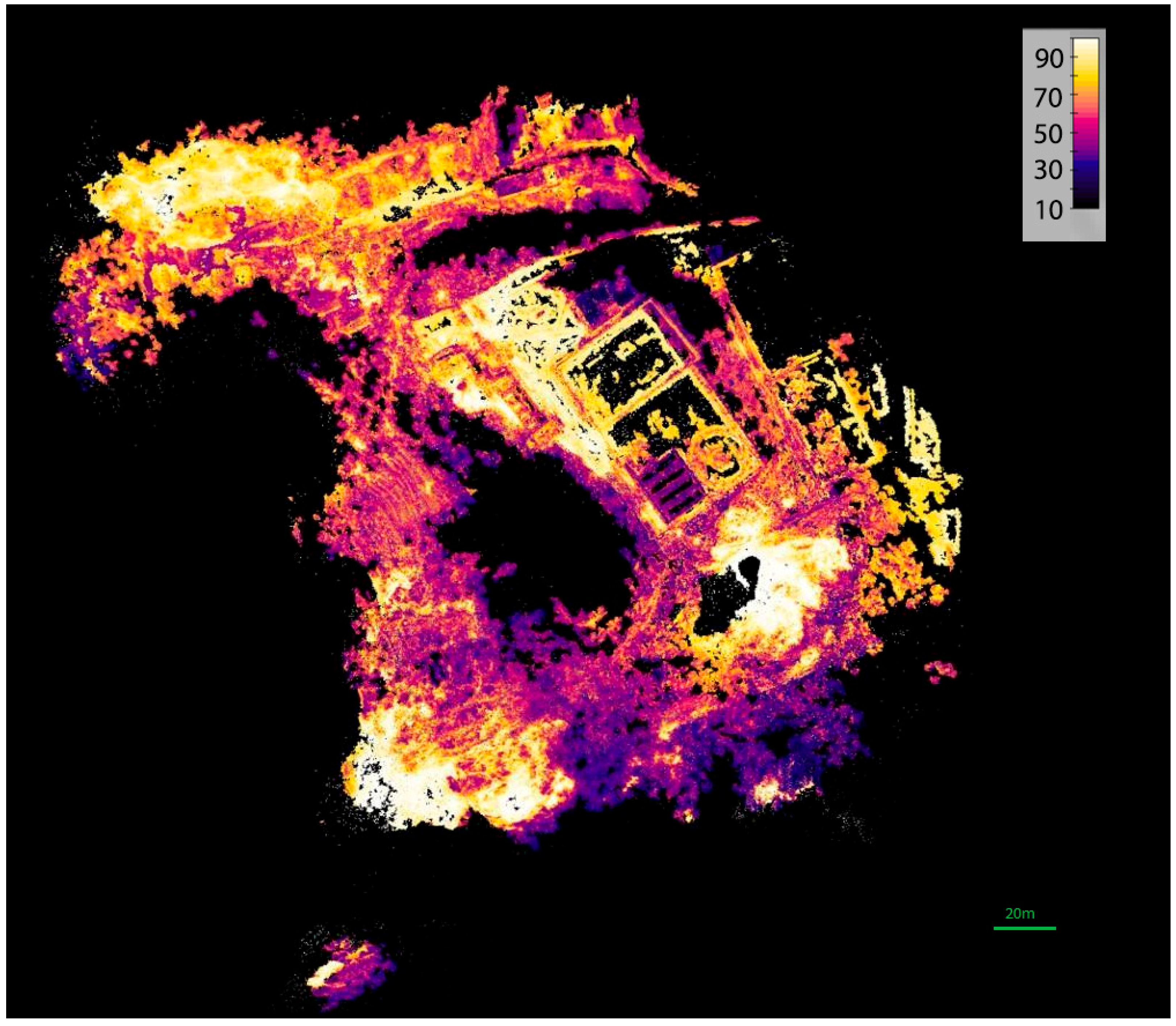
Figure 4.
Thermal 3D point cloud of the Pisciarelli area. The colours represent temperatures as in the shown scale.
Figure 4.
Thermal 3D point cloud of the Pisciarelli area. The colours represent temperatures as in the shown scale.
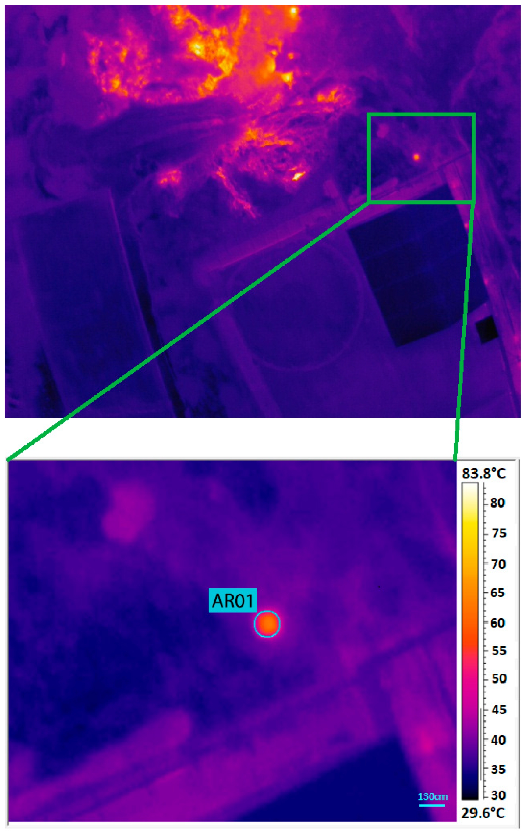
Figure 5.
Details of the 3D thermal mesh of 14 September 2020. The red square identifies the tie point related to a manhole, with the number of images marked on the right. The colours represent temperatures as in the shown scale in
Figure 4. The images on the right-hand side are the single thermal images, where the tie point is identified.
Figure 6.
Details of the Index Map of 8 March 2021 at a height of 70 m, with temperature intervals between 25 and 35 °C. In (a), an artificial thermal target, DTT. In (b), a natural thermal anomaly, a manhole NTT. The grey background represents the temperatures in the not-indexed pixels.
Figure 6.
Details of the Index Map of 8 March 2021 at a height of 70 m, with temperature intervals between 25 and 35 °C. In (a), an artificial thermal target, DTT. In (b), a natural thermal anomaly, a manhole NTT. The grey background represents the temperatures in the not-indexed pixels.
Figure 7.
Top, the original thermal frame acquired via UAS. Bottom, recognition of the thermal target on individual frames. This case is the manhole of the NTT, reconstructed using a circular geometric shape.
Figure 7.
Top, the original thermal frame acquired via UAS. Bottom, recognition of the thermal target on individual frames. This case is the manhole of the NTT, reconstructed using a circular geometric shape.
Figure 8.
(a) digital surface model (DSM) of the geothermal Pisciarelli area with an overlaid thermal map; (b) details of the thermal map in the GIS environment. The red circles highlight the NTT identified on the map related to the flight of 14 September. The colours on the map represent the temperatures in °C as in the scale in the legend.
Figure 9.
(a) digital surface model (DSM) of the geothermal Pisciarelli area with an overlaid thermal map; (b) details of thermal map in the GIS environment. The red circles highlight the DTT and NTT identified on the map related to flight of 8 March at a height of 55 m. The colours on the map represent the temperatures in °C as in the scale in the legend.
Figure 10.
(a) Thermal image of the joint DTT set at 50 °C. The box highlights the areas where temperatures have been calculated. (b) Image of joint DTT in RGB.
Figure 10.
(a) Thermal image of the joint DTT set at 50 °C. The box highlights the areas where temperatures have been calculated. (b) Image of joint DTT in RGB.
Table 1.
Main characteristics of the UAS’s radiometric thermal camera Vue PRO R.
Table 1.
Main characteristics of the UAS’s radiometric thermal camera Vue PRO R.
| Model | Vue PRO R |
|---|
| Sensor Technology | Uncooled Vox Microbolometer |
| Weight | 92–113.4 g |
| Size | 57.4 × 44.45 × 44.45 mm (including lens) |
| Lens Options (FOV for Full-Sensor Digital Output) | 9 mm 69° × 56° |
| Resolution | 640 × 512 pixel |
| Spectral band | 7.5–13.5 μm |
| Full Frame Rates | 30 Hz (NTSC 1); 25 Hz (PAL 2) |
| Measurement Accuracy | +/−5 °C or 5% of reading |
| Accuracy | +/−5 °C o 5% of reading in −25 °C to +135 °C range |
| | +/−20 °C or 20% of reading in −40 °C to +550 °C range |
| Radiometric Data | Yes |
Table 2.
Weighted average and error on NTT points of a single thermal target for the survey of 14 September at 70 m height. T1 is the weighted average calculated with ThermaCAM Researcher over each single frame, and T2 is the average temperature calculated based on the thermal map in GIS.
Table 2.
Weighted average and error on NTT points of a single thermal target for the survey of 14 September at 70 m height. T1 is the weighted average calculated with ThermaCAM Researcher over each single frame, and T2 is the average temperature calculated based on the thermal map in GIS.
| Point | n° of Frame | T1 (°C) ± σ | T2 (°C) ± σ | ∣T1 − T2∣(°C) ± σ |
|---|
| AR01 | 17 | 44.8 ± 0.2 | 46 ± 7 | 1 ± 7 |
| AR02 | 10 | 33.36 ± 0.01 | 33.0 ± 0.6 | 0.3 ± 0.6 |
| AR03 | 5 | 28.82 ± 0.02 | 27.2 ± 0.5 | 1.6 ± 0.5 |
| AR04 | 20 | 53.98 ± 0.02 | 53 ± 5 | 1 ± 5 |
| AR05 | 3 | 70.57 ± 0.04 | 64 ± 9 | 6 ± 9 |
Table 3.
Weighted average and error on DTT and NTT points of a single thermal frame for the survey of 8 March, at a 70 m height, highlighted on thermal map in the 25–35 °C interval. T1 is the weighted average calculated with ThermaCAM Researcher using each single frame, and T2 is the average temperature calculated based on the thermal map in GIS.
| Point | n° of Frame | T1 (°C) ± σ | T2 (°C) ± σ | ∣T1 − T2∣ (°C) ± σ |
|---|
| DTT | 26 | 28.2 ± 0.3 | 30 ± 2 | 1 ± 2 |
| NTT | 8 | 27.6 ± 0.3 | 27 ± 3 | 1 ± 3 |
Table 4.
Weighted average and error on DTT and NTT points of a single thermal frame for the survey of 8 March, at 55 m height. T1 is the weighted average calculated with ThermaCAM Researcher using single frames, and T2 is the average temperature calculated based on the thermal map in GIS.
Table 4.
Weighted average and error on DTT and NTT points of a single thermal frame for the survey of 8 March, at 55 m height. T1 is the weighted average calculated with ThermaCAM Researcher using single frames, and T2 is the average temperature calculated based on the thermal map in GIS.
| Point | n° of Frame | T1 (°C) ± σ | T2 (°C) ± σ | ∣T1 − T2∣(°C) ± σ |
|---|
| DTT | 28 | 30.50 ± 0.02 | 32 ± 2 | 1 ± 2 |
| NTT | 8 | 27.4 ± 0.3 | 25 ± 3 | 2 ± 3 |
Table 5.
Temperature differences between the various temperatures measured for the manhole and the DTT at the different heights.
Table 5.
Temperature differences between the various temperatures measured for the manhole and the DTT at the different heights.
| Δh (m) | ΔT (°C) | Variation (°C/m) |
|---|
| DTT |
| 54 | 10 ± 4 | 0.19 ± 0.07 |
| 69 | 12 ± 4 | 0.17 ± 0.06 |
| DTT—weighted average decrease | 0.18 ± 0.05 |
| Manhole |
| 54 | 15 ± 8 | 0.28 ± 0.14 |
| 69 | 13 ± 8 | 0.19 ± 0.12 |
| 15 | 2 ± 6 | 0.1 ± 0.4 |
| Manhole—weighted average variation | 0.22 ± 0.09 |
| Compound weighted average variation | 0.19 ± 0.04 |
| Disclaimer/Publisher’s Note: The statements, opinions and data contained in all publications are solely those of the individual author(s) and contributor(s) and not of MDPI and/or the editor(s). MDPI and/or the editor(s) disclaim responsibility for any injury to people or property resulting from any ideas, methods, instructions or products referred to in the content. |
© 2023 by the authors. Licensee MDPI, Basel, Switzerland. This article is an open access article distributed under the terms and conditions of the Creative Commons Attribution (CC BY) license (https://creativecommons.org/licenses/by/4.0/).


 ,
, 


