
CCC-SSA-UNet: U-Shaped Pansharpening Network with Channel Cross-Concatenation and Spatial–Spectral Attention Mechanism for Hyperspectral Image Super-Resolution

 , ,
, ,  and
and
Abstract
:
1. Introduction
- We propose a novel framework for hyperspectral pansharpening named the CCC-SSA-UNet, which integrates the UNet architecture with the SSA-Net.
- We propose a novel channel cross-concatenation method called Input CCC at the network’s entrance. This method effectively enhances the fusion capability of different input source images while introducing only a minimal number of additional parameters. Furthermore, we propose a Feature CCC approach within the decoder. This approach effectively strengthens the fusion capacity between different hierarchical feature maps without introducing any extra parameters or computational complexity.
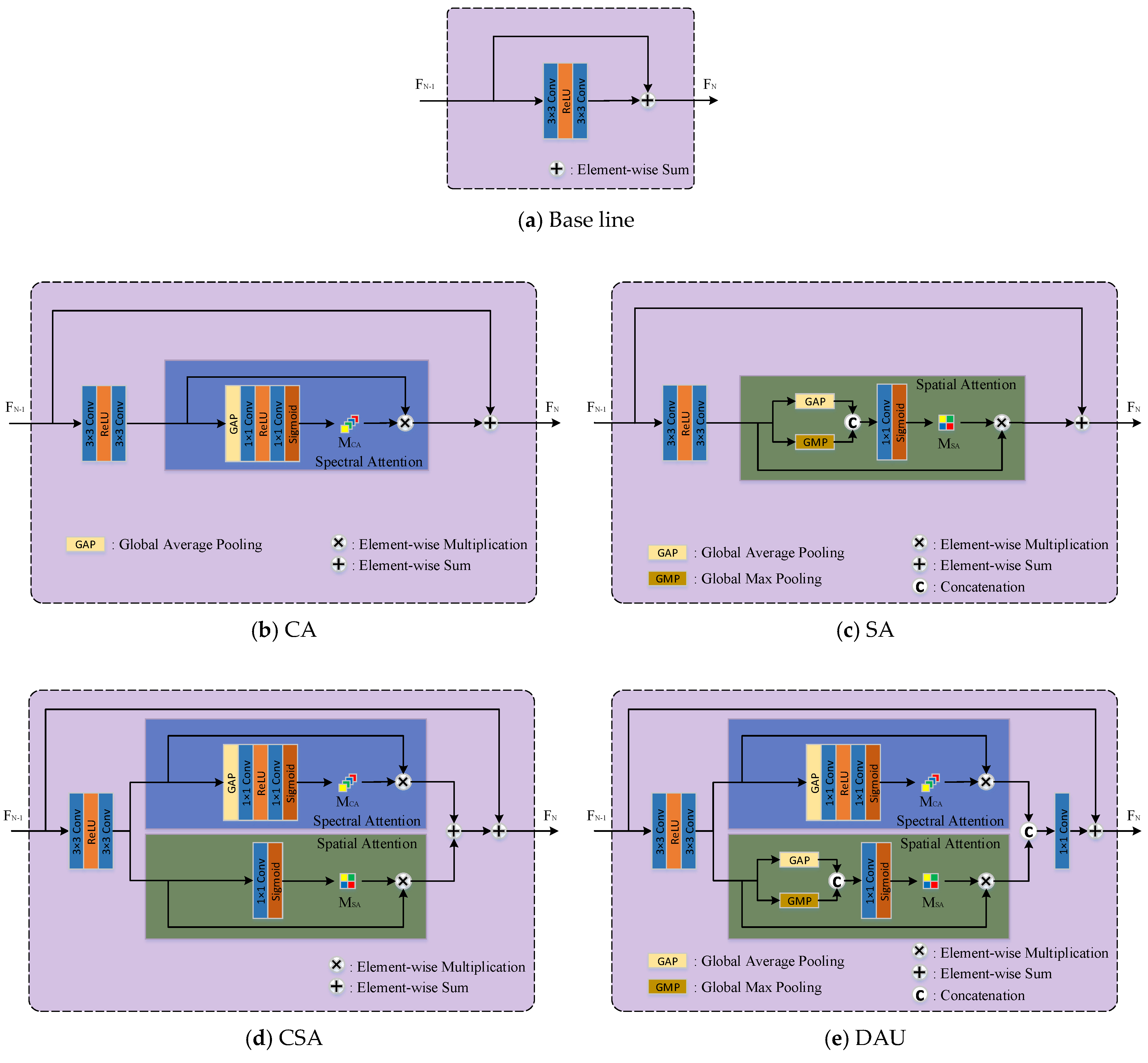
- We propose an improved Res-SSA block to enhance the representation capacity of spatial and spectral features. Experimental results demonstrate the effectiveness of our proposed hybrid attention module and its superiority over other attention module variants.
2. Related Work
2.1. Classical Pansharpening Methods
2.2. Deep Learning-Based Pansharpening Methods
3. Proposed Method
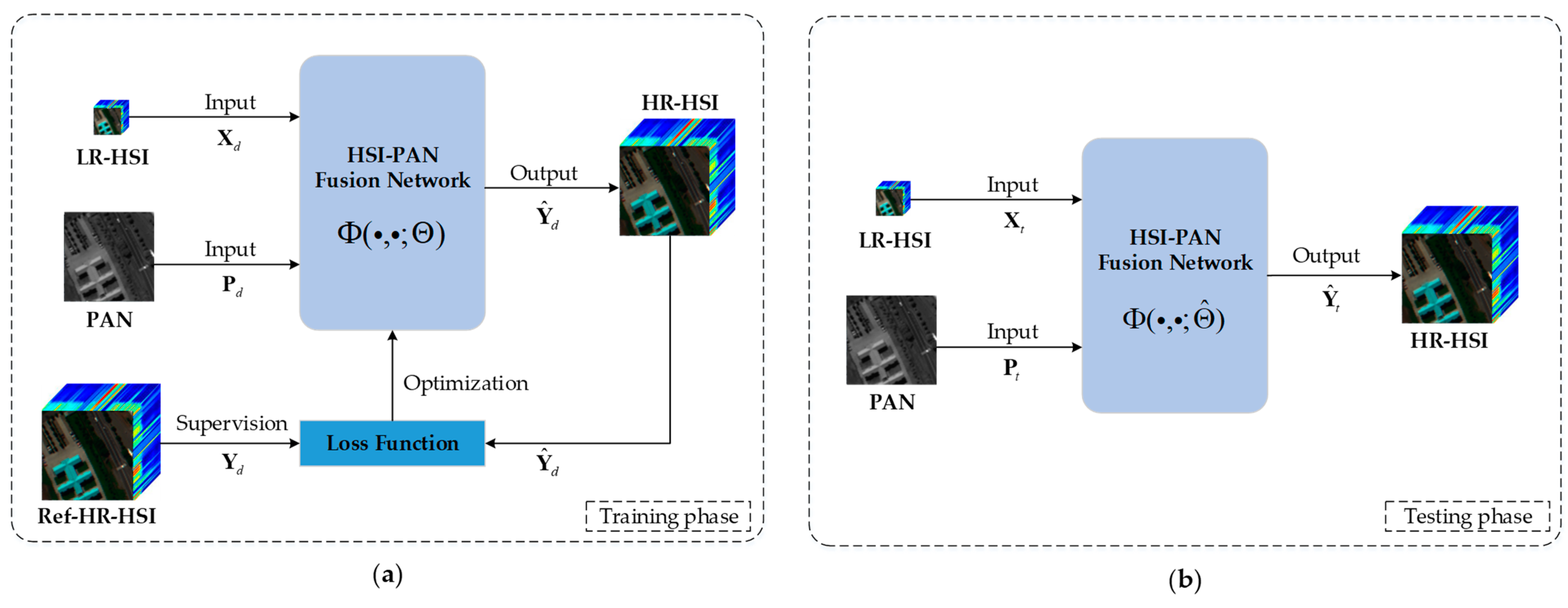
3.1. Problem Statement and Formulation
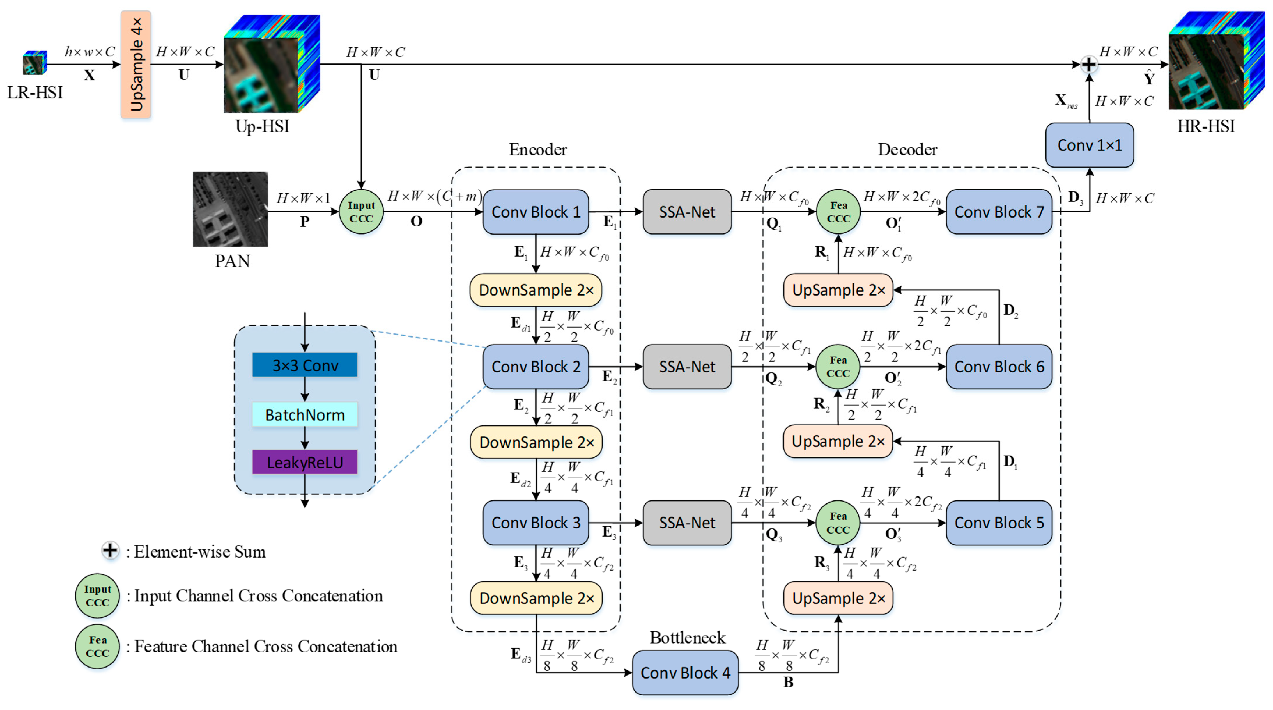
3.2. Network Design
3.2.1. UNet Backbone
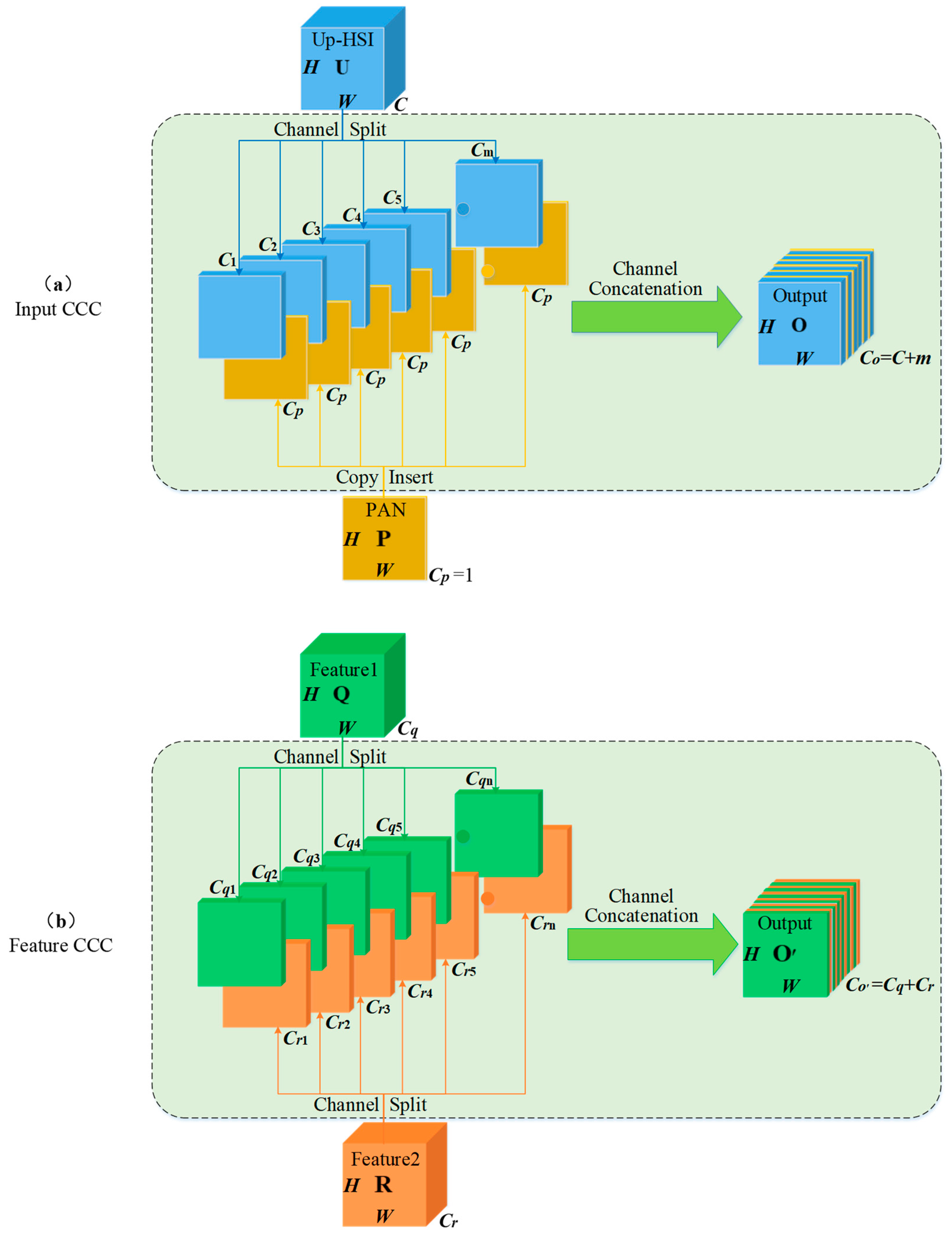
3.2.2. CCC
- Input CCC
- Feature CCC
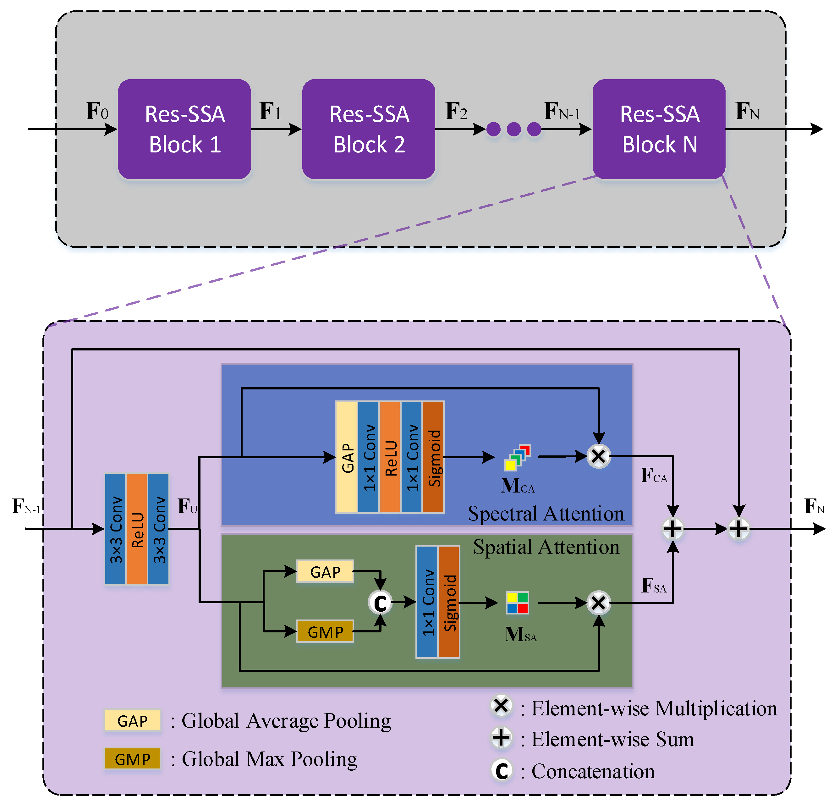
3.2.3. SSA-Net
3.3. Loss Function
4. Experiments and Discussion
4.1. Datasets
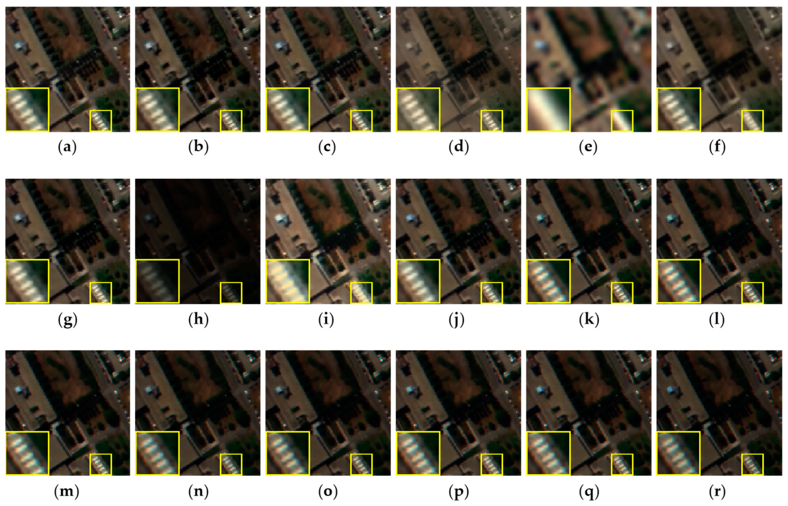
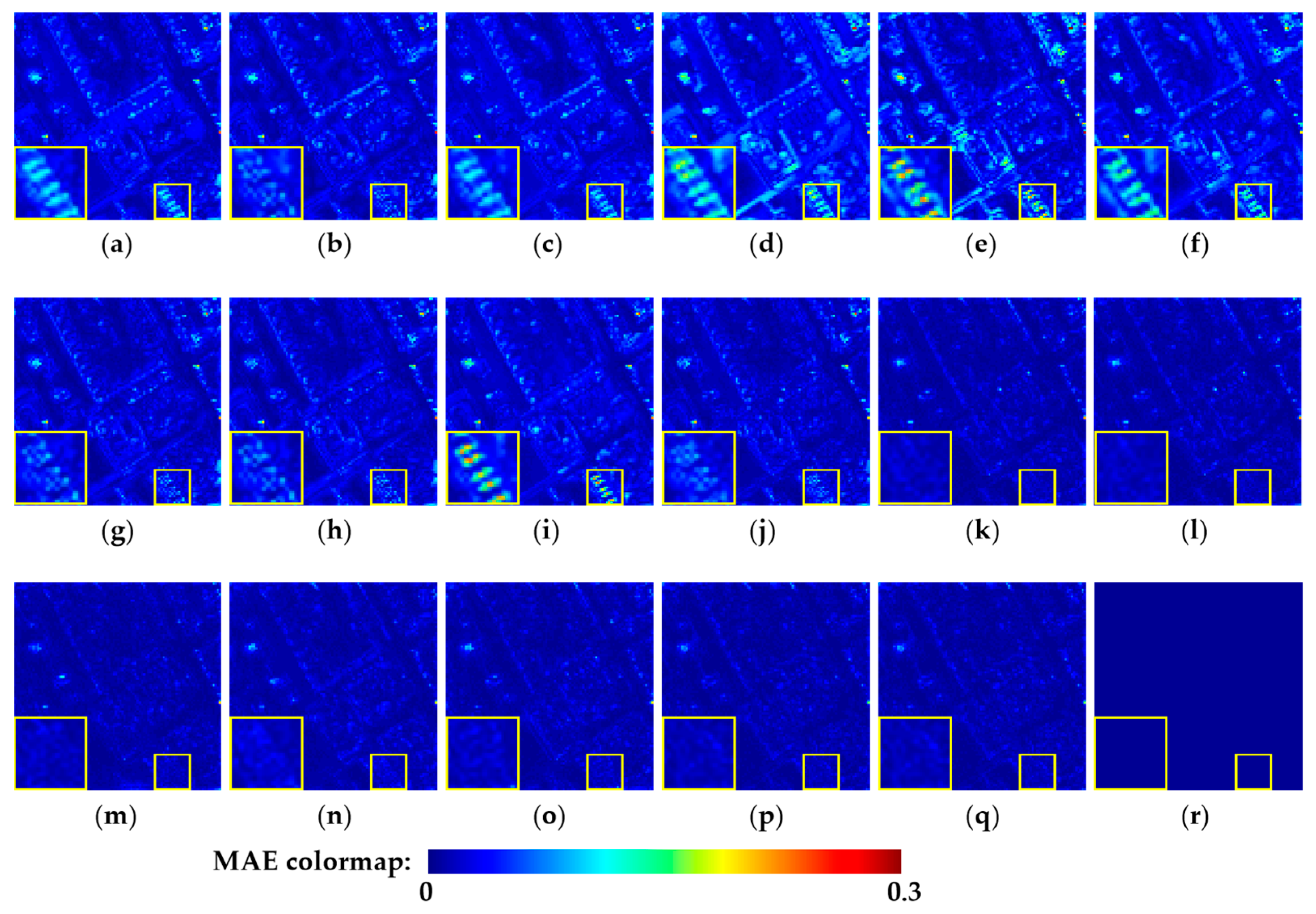
- Pavia University Dataset [61]: The Pavia University dataset comprises aerial images acquired over Pavia University in Italy, utilizing the Reflective Optics System Imaging Spectrometer (ROSIS). The original image has a spatial resolution of 1.3 m and dimensions of 610 × 610 pixels. The ROSIS sensor captures 115 spectral bands, covering the spectral range of 430–860 nm. After excluding noisy bands, the image dataset contains 103 spectral bands. To remove uninformative regions, the right-side portion of the image was cropped, leaving a 610 × 340 pixel area for further analysis. Subsequently, a non-overlapping region of 576 × 288 pixels, situated at the top-left corner, was extracted and divided into 18 sub-images measuring 96 × 96 pixels each. These sub-images constitute the reference HR-HSI dataset, serving as the ground truth. To generate corresponding PAN and LR-HSI, the Wald protocol [62] was employed. Specifically, a Gaussian filter with an 8 × 8 kernel size was applied to blur the HR-HSI, followed by a downsampling process, reducing its spatial dimensions by a factor of four to obtain the LR-HSI. The PAN was created by computing the average of the first 100 spectral bands of the HR-HSI. Fourteen image pairs were randomly selected for the training set, while the remaining four pairs were reserved for the test set.
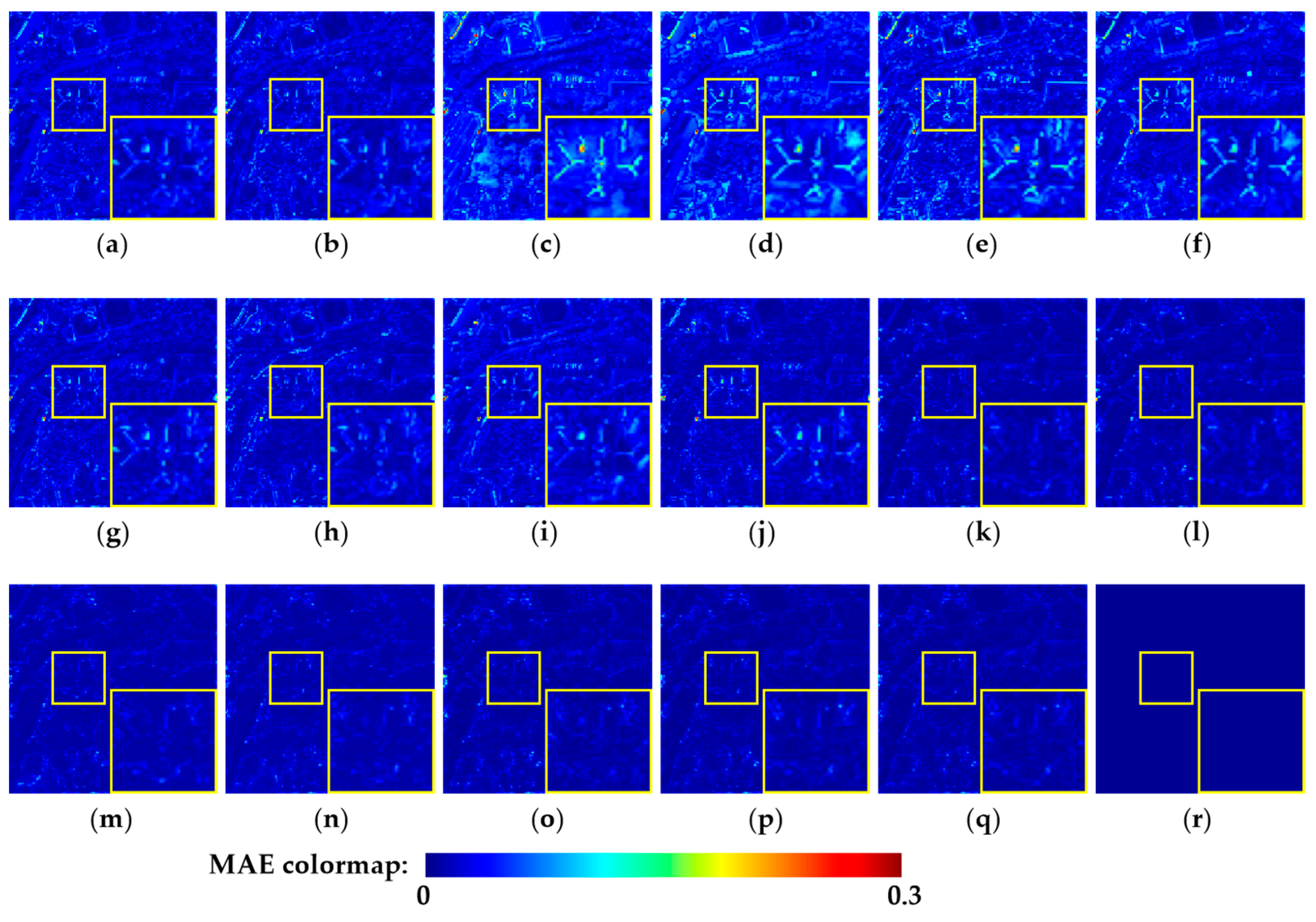
- Pavia Centre Dataset [61]: The Pavia Centre dataset consists of aerial images captured over the city center of Pavia, located in northern Italy, using the Reflective Optics System Imaging Spectrometer (ROSIS). The original image has dimensions of 1096 × 1096 pixels and a spatial resolution of 1.3 m, similar to the Pavia University dataset. After excluding 13 noisy bands, the dataset contains 102 spectral bands, covering the spectral range of 430–860 nm. Due to the lack of informative content in the central region of the image, this portion was cropped, and only the remaining 1096 × 715 pixel area containing the relevant information was used for analysis. Subsequently, a non-overlapping region of 960 × 640 pixels, situated at the top-left corner, was extracted and divided into 24 sub-images measuring 160 × 160 pixels each. These sub-images constitute the reference HR-HSI dataset, serving as the ground truth. Similar to the Pavia University Dataset, the PAN and LR-HSI corresponding to the HR-HSI were generated using the same methodology. Eighteen image pairs were randomly selected as the training set, while the remaining seven pairs were designated as the test set.
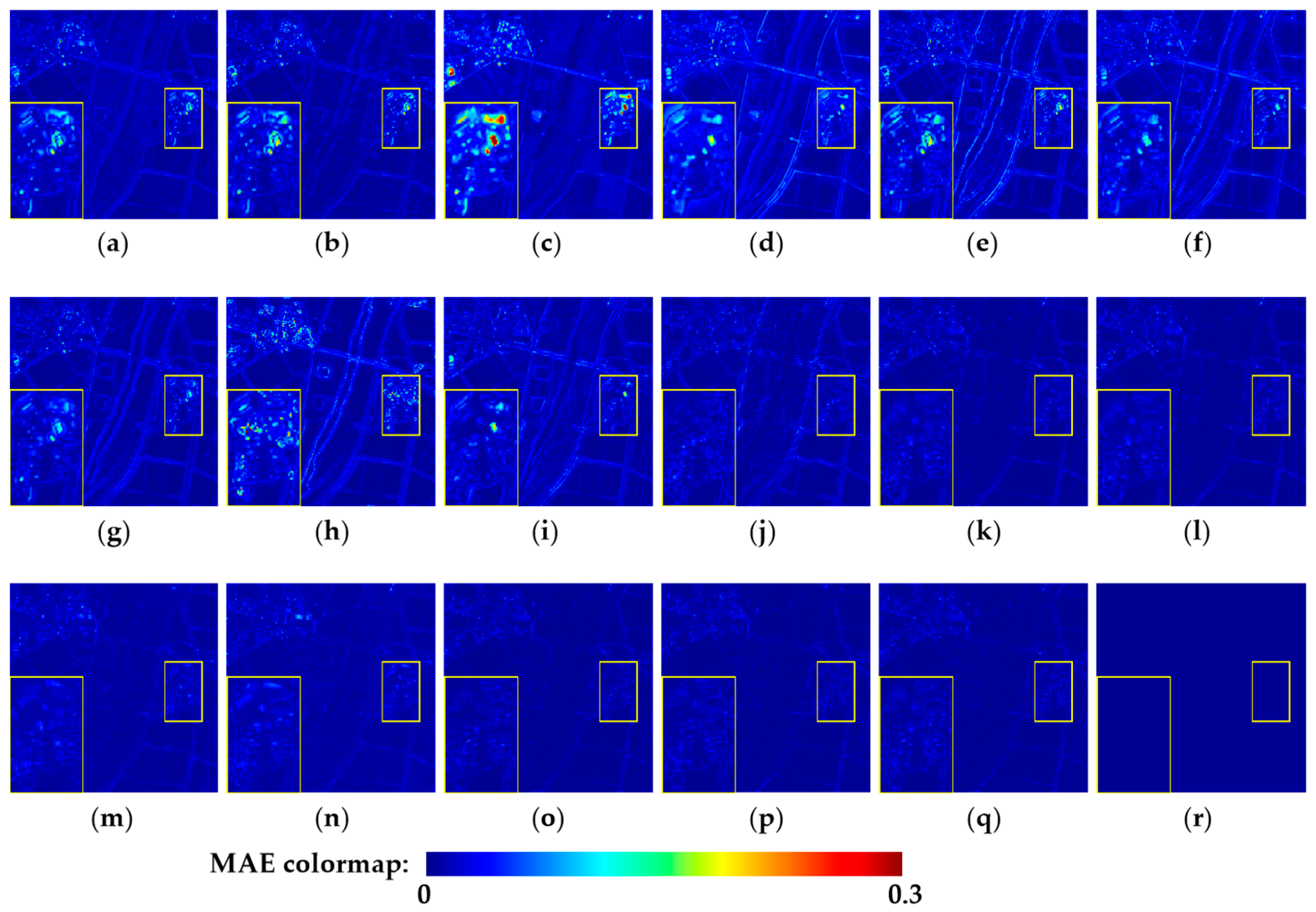
- Chikusei Dataset [63]: The Chikusei dataset comprises aerial images captured over the agricultural and urban areas of Chikusei, Japan, in 2014, using the Headwall Hyperspec-VNIR-C sensor. The original image has pixel dimensions of 2517 × 2355 and a spatial resolution of 2.5 m. It encompasses a total of 128 spectral bands, covering the spectral range of 363–1018 nm. For the experiments, a non-overlapping region of 2304 × 2304 pixels was selected from the top-left corner and divided into 81 sub-images of 256 × 256 pixels. These sub-images constitute the reference HR-HSI dataset, serving as the ground truth. Similar to the Pavia University dataset, LR-HSI corresponding to the HR-HSI were generated using the same method. The PAN image was obtained by averaging the spectral bands from 60 to 100 of the HR-HSI. Sixty-one image pairs were randomly selected as the training set, while the remaining 20 pairs were allocated to the test set.
4.2. Evaluation Metrics
4.3. Implementation Details
4.4. Comparison with State-of-the-Art Methods
4.4.1. Experiments on Pavia University Dataset
4.4.2. Experiments on Pavia Centre Dataset
4.4.3. Experiments on Chikusei Dataset
4.5. Analysis of the Computational Complexity
4.6. Sensitivity Analysis of the Network Parameters
4.6.1. Analysis of the Filter Channel Numbers
4.6.2. Analysis of the Input CCC Group Numbers
4.6.3. Analysis of the Feature CCC Group Numbers
4.6.4. Analysis of the SSA Block Numbers
4.6.5. Analysis of the Learning Rate
4.7. Ablation Study
4.7.1. Effect of the Proposed Input CCC
4.7.2. Effect of the Proposed Feature CCC
4.7.3. Effect of the Proposed SSA-Net
4.7.4. Effect of the Proposed Res-SSA Block
5. Conclusions
Author Contributions
Funding
Data Availability Statement
Acknowledgments
Conflicts of Interest
References
- Audebert, N.; Saux, B.L.; Lefevre, S. Deep Learning for Classification of Hyperspectral Data: A Comparative Review. IEEE Geosci. Remote Sens. Mag. 2019, 7, 159–173. [Google Scholar] [CrossRef]
- Fabelo, H.; Ortega, S.; Ravi, D.; Kiran, B.R.; Sosa, C.; Bulters, D.; Callicó, G.M.; Bulstrode, H.; Szolna, A.; Piñeiro, J.F.; et al. Spatio-spectral classification of hyperspectral images for brain cancer detection during surgical operations. PLoS ONE 2018, 13, e0193721. [Google Scholar] [CrossRef] [PubMed]
- Xie, W.; Lei, J.; Fang, S.; Li, Y.; Jia, X.; Li, M. Dual feature extraction network for hyperspectral image analysis. Pattern Recognit. 2021, 118, 107992. [Google Scholar] [CrossRef]
- Zhang, M.; Sun, X.; Zhu, Q.; Zheng, G. A Survey of Hyperspectral Image Super-Resolution Technology. In Proceedings of the 2021 IEEE International Geoscience and Remote Sensing Symposium IGARSS, Brussels, Belgium, 11–16 July 2021; pp. 4476–4479. [Google Scholar]
- Laben, C.A.; Brower, B.V. Process for Enhancing the Spatial Resolution of Multispectral Imagery Using Pan-Sharpening. U.S. Patent 6,011,875, 4 January 2000. [Google Scholar]
- Aiazzi, B.; Baronti, S.; Selva, M. Improving Component Substitution Pansharpening through Multivariate Regression of MS + Pan Data. IEEE Trans. Geosci. Remote Sens. 2007, 45, 3230–3239. [Google Scholar] [CrossRef]
- Liao, W.; Huang, X.; Van Coillie, F.; Gautama, S.; Pižurica, A.; Philips, W.; Liu, H.; Zhu, T.; Shimoni, M.; Moser, G. Processing of multiresolution thermal hyperspectral and digital color data: Outcome of the 2014 IEEE GRSS data fusion contest. IEEE J. Sel. Top. Appl. Earth Obs. Remote Sens. 2015, 8, 2984–2996. [Google Scholar] [CrossRef]
- Shah, V.P.; Younan, N.H.; King, R.L. An Efficient Pan-Sharpening Method via a Combined Adaptive PCA Approach and Contourlets. IEEE Trans. Geosci. Remote Sens. 2008, 46, 1323–1335. [Google Scholar] [CrossRef]
- Aiazzi, B.; Alparone, L.; Baronti, S.; Garzelli, A.; Selva, M. MTF-tailored multiscale fusion of high-resolution MS and Pan imagery. Photogramm. Eng. Remote Sens. 2006, 72, 591–596. [Google Scholar] [CrossRef]
- Liu, J. Smoothing filter-based intensity modulation: A spectral preserve image fusion technique for improving spatial details. Int. J. Remote Sens. 2000, 21, 3461–3472. [Google Scholar] [CrossRef]
- Vivone, G.; Restaino, R.; Mura, M.D.; Licciardi, G.; Chanussot, J. Contrast and Error-Based Fusion Schemes for Multispectral Image Pansharpening. IEEE Geosci. Remote Sens. Lett. 2014, 11, 930–934. [Google Scholar] [CrossRef]
- Simões, M.; Bioucas-Dias, J.; Almeida, L.B.; Chanussot, J. A Convex Formulation for Hyperspectral Image Superresolution via Subspace-Based Regularization. IEEE Trans. Geosci. Remote Sens. 2015, 53, 3373–3388. [Google Scholar] [CrossRef]
- Wei, Q.; Bioucas-Dias, J.; Dobigeon, N.; Tourneret, J.Y. Hyperspectral and Multispectral Image Fusion Based on a Sparse Representation. IEEE Trans. Geosci. Remote Sens. 2015, 53, 3658–3668. [Google Scholar] [CrossRef]
- Wei, Q.; Dobigeon, N.; Tourneret, J.Y. Bayesian Fusion of Multi-Band Images. IEEE J. Sel. Top. Signal Process. 2015, 9, 1117–1127. [Google Scholar] [CrossRef]
- Kawakami, R.; Matsushita, Y.; Wright, J.; Ben-Ezra, M.; Tai, Y.; Ikeuchi, K. High-resolution hyperspectral imaging via matrix factorization. In Proceedings of the CVPR 2011, Colorado Springs, CO, USA, 20–25 June 2011; pp. 2329–2336. [Google Scholar]
- Yokoya, N.; Yairi, T.; Iwasaki, A. Coupled Nonnegative Matrix Factorization Unmixing for Hyperspectral and Multispectral Data Fusion. IEEE Trans. Geosci. Remote Sens. 2012, 50, 528–537. [Google Scholar] [CrossRef]
- Tan, M.; Pang, R.; Le, Q.V. Efficientdet: Scalable and efficient object detection. In Proceedings of the IEEE/CVF Conference on Computer Vision and Pattern Recognition, Seattle, WA, USA, 13–19 June 2020; pp. 10781–10790. [Google Scholar]
- Zhang, Z.; Lu, X.; Cao, G.; Yang, Y.; Jiao, L.; Liu, F. ViT-YOLO: Transformer-Based YOLO for Object Detection. In Proceedings of the IEEE/CVF International Conference on Computer Vision (ICCV) Workshops, Montreal, BC, Canada, 11–17 October 2021; pp. 2799–2808. [Google Scholar]
- Cao, Z.; Fu, C.; Ye, J.; Li, B.; Li, Y. SiamAPN++: Siamese Attentional Aggregation Network for Real-Time UAV Tracking. In Proceedings of the 2021 IEEE/RSJ International Conference on Intelligent Robots and Systems (IROS), Prague, Czech Republic, 27 September–1 October 2021; pp. 3086–3092. [Google Scholar]
- Zhang, G.; Li, Z.; Li, J.; Hu, X. CFNet: Cascade Fusion Network for Dense Prediction. arXiv 2023, arXiv:2302.06052. [Google Scholar]
- Zhang, K.; Li, Y.; Liang, J.; Cao, J.; Zhang, Y.; Tang, H.; Timofte, R.; Van Gool, L. Practical Blind Denoising via Swin-Conv-UNet and Data Synthesis. arXiv 2022, arXiv:2203.13278. [Google Scholar]
- Cho, S.-J.; Ji, S.-W.; Hong, J.-P.; Jung, S.-W.; Ko, S.-J. Rethinking coarse-to-fine approach in single image deblurring. In Proceedings of the 2021 IEEE/CVF International Conference on Computer Vision (ICCV), Montreal, QC, Canada, 10–17 October 2021; pp. 4641–4650. [Google Scholar]
- Liang, J.; Cao, J.; Sun, G.; Zhang, K.; Gool, L.V.; Timofte, R. SwinIR: Image Restoration Using Swin Transformer. In Proceedings of the 2021 IEEE/CVF International Conference on Computer Vision Workshops (ICCVW), Montreal, BC, Canada, 11–17 October 2021; pp. 1833–1844. [Google Scholar]
- Wang, X.; Xie, L.; Dong, C.; Shan, Y. Real-ESRGAN: Training Real-World Blind Super-Resolution with Pure Synthetic Data. In Proceedings of the IEEE/CVF International Conference on Computer Vision, Montreal, BC, Canada, 11–17 October 2021; pp. 1905–1914. [Google Scholar]
- Wang, X.; Yu, K.; Wu, S.; Gu, J.; Liu, Y.; Dong, C.; Qiao, Y.; Change Loy, C. ESRGAN: Enhanced Super-Resolution Generative Adversarial Networks. In Proceedings of the European Conference on Computer Vision (ECCV) Workshops, Munich, Germany, 8–14 September 2018. [Google Scholar]
- Yoo, J.; Kim, T.; Lee, S.; Kim, S.H.; Lee, H.; Kim, T.H. Enriched CNN-Transformer Feature Aggregation Networks for Super-Resolution. In Proceedings of the IEEE/CVF Winter Conference on Applications of Computer Vision (WACV), Waikoloa, HI, USA, 2–7 January 2023; pp. 4956–4965. [Google Scholar]
- Zhang, Y.; Li, K.; Li, K.; Wang, L.; Zhong, B.; Fu, Y. Image Super-Resolution Using Very Deep Residual Channel Attention Networks. In Proceedings of the European Conference on Computer Vision (ECCV), Munich, Germany, 8–14 September 2018; pp. 286–301. [Google Scholar]
- He, L.; Zhu, J.; Li, J.; Plaza, A.; Chanussot, J.; Li, B. HyperPNN: Hyperspectral Pansharpening via Spectrally Predictive Convolutional Neural Networks. IEEE J. Sel. Top. Appl. Earth Obs. Remote Sens. 2019, 12, 3092–3100. [Google Scholar] [CrossRef]
- Zhuo, Y.W.; Zhang, T.J.; Hu, J.F.; Dou, H.X.; Huang, T.Z.; Deng, L.J. A Deep-Shallow Fusion Network With Multidetail Extractor and Spectral Attention for Hyperspectral Pansharpening. IEEE J. Sel. Top. Appl. Earth Obs. Remote Sens. 2022, 15, 7539–7555. [Google Scholar] [CrossRef]
- Zheng, Y.; Li, J.; Li, Y.; Guo, J.; Wu, X.; Chanussot, J. Hyperspectral Pansharpening Using Deep Prior and Dual Attention Residual Network. IEEE Trans. Geosci. Remote Sens. 2020, 58, 8059–8076. [Google Scholar] [CrossRef]
- Bandara, W.G.C.; Valanarasu, J.M.J.; Patel, V.M. Hyperspectral Pansharpening Based on Improved Deep Image Prior and Residual Reconstruction. IEEE Trans. Geosci. Remote Sens. 2022, 60, 1–16. [Google Scholar] [CrossRef]
- Dong, W.; Hou, S.; Xiao, S.; Qu, J.; Du, Q.; Li, Y. Generative Dual-Adversarial Network With Spectral Fidelity and Spatial Enhancement for Hyperspectral Pansharpening. IEEE Trans. Neural Netw. Learn. Syst. 2021, 33, 7303–7317. [Google Scholar] [CrossRef]
- Xie, W.; Cui, Y.; Li, Y.; Lei, J.; Du, Q.; Li, J. HPGAN: Hyperspectral Pansharpening Using 3-D Generative Adversarial Networks. IEEE Trans. Geosci. Remote Sens. 2021, 59, 463–477. [Google Scholar] [CrossRef]
- Bandara, W.G.C.; Patel, V.M. HyperTransformer: A Textural and Spectral Feature Fusion Transformer for Pansharpening. In Proceedings of the IEEE/CVF Conference on Computer Vision and Pattern Recognition, New Orleans, LA, USA, 18–24 June 2022; pp. 1767–1777. [Google Scholar]
- He, L.; Xi, D.; Li, J.; Lai, H.; Plaza, A.; Chanussot, J. Dynamic Hyperspectral Pansharpening CNNs. IEEE Trans. Geosci. Remote Sens. 2023, 61, 1–19. [Google Scholar] [CrossRef]
- Luo, F.; Zhou, T.; Liu, J.; Guo, T.; Gong, X.; Ren, J. Multiscale Diff-Changed Feature Fusion Network for Hyperspectral Image Change Detection. IEEE Trans. Geosci. Remote Sens. 2023, 61, 5502713. [Google Scholar] [CrossRef]
- He, X.; Tang, C.; Liu, X.; Zhang, W.; Sun, K.; Xu, J. Object Detection in Hyperspectral Image via Unified Spectral-Spatial Feature Aggregation. arXiv 2023, arXiv:2306.08370. [Google Scholar]
- Kordi Ghasrodashti, E. Hyperspectral image classification using a spectral–spatial random walker method. Int. J. Remote Sens. 2019, 40, 3948–3967. [Google Scholar] [CrossRef]
- Chavez, P.; Sides, S.C.; Anderson, J.A. Comparison of three different methods to merge multiresolution and multispectral data-Landsat TM and SPOT panchromatic. Photogramm. Eng. Remote Sens. 1991, 57, 295–303. [Google Scholar]
- Burt, P.J.; Adelson, E.H. The Laplacian pyramid as a compact image code. In Readings in Computer Vision; Fischler, M.A., Firschein, O., Eds.; Morgan Kaufmann: San Francisco, CA, USA, 1987; pp. 671–679. [Google Scholar]
- Aiazzi, B.; Alparone, L.; Baronti, S.; Garzelli, A. Context-driven fusion of high spatial and spectral resolution images based on oversampled multiresolution analysis. IEEE Trans. Geosci. Remote Sens. 2002, 40, 2300–2312. [Google Scholar] [CrossRef]
- Dong, W.; Zhang, T.; Qu, J.; Xiao, S.; Liang, J.; Li, Y. Laplacian Pyramid Dense Network for Hyperspectral Pansharpening. IEEE Trans. Geosci. Remote Sens. 2022, 60, 5507113. [Google Scholar] [CrossRef]
- Fasbender, D.; Radoux, J.; Bogaert, P. Bayesian Data Fusion for Adaptable Image Pansharpening. IEEE Trans. Geosci. Remote Sens. 2008, 46, 1847–1857. [Google Scholar] [CrossRef]
- Wei, Q.; Dobigeon, N.; Tourneret, J. Fast Fusion of Multi-Band Images Based on Solving a Sylvester Equation. IEEE Trans. Image Process. 2015, 24, 4109–4121. [Google Scholar] [CrossRef]
- Xue, J.; Zhao, Y.Q.; Bu, Y.; Liao, W.; Chan, J.C.W.; Philips, W. Spatial-Spectral Structured Sparse Low-Rank Representation for Hyperspectral Image Super-Resolution. IEEE Trans. Image Process. 2021, 30, 3084–3097. [Google Scholar] [CrossRef] [PubMed]
- Masi, G.; Cozzolino, D.; Verdoliva, L.; Scarpa, G. Pansharpening by convolutional neural networks. Remote Sens. 2016, 8, 594. [Google Scholar] [CrossRef]
- Yuan, Q.; Wei, Y.; Meng, X.; Shen, H.; Zhang, L. A Multiscale and Multidepth Convolutional Neural Network for Remote Sensing Imagery Pan-Sharpening. IEEE J. Sel. Top. Appl. Earth Obs. Remote Sens. 2018, 11, 978–989. [Google Scholar] [CrossRef]
- Liu, X.; Liu, Q.; Wang, Y. Remote sensing image fusion based on two-stream fusion network. Inf. Fusion 2020, 55, 1–15. [Google Scholar] [CrossRef]
- Hu, J.; Shen, L.; Sun, G. Squeeze-and-Excitation Networks. In Proceedings of the 2018 IEEE/CVF Conference on Computer Vision and Pattern Recognition (CVPR), Salt Lake City, UT, USA, 18–23 June 2018; pp. 7132–7141. [Google Scholar]
- Roy, A.G.; Navab, N.; Wachinger, C. Concurrent spatial and channel ‘squeeze & excitation’ in fully convolutional networks. In Proceedings of the International Conference on Medical Image Computing and Computer-Assisted Intervention, Granada, Spain, 16–20 September 2018; pp. 421–429. [Google Scholar]
- Ronneberger, O.; Fischer, P.; Brox, T. U-net: Convolutional networks for biomedical image segmentation. In Proceedings of the Medical Image Computing and Computer-Assisted Intervention–MICCAI 2015: 18th International Conference, Munich, Germany, 5–9 October 2015; pp. 234–241. [Google Scholar]
- Bass, C.; Silva, M.d.; Sudre, C.; Williams, L.Z.J.; Sousa, H.S.; Tudosiu, P.D.; Alfaro-Almagro, F.; Fitzgibbon, S.P.; Glasser, M.F.; Smith, S.M.; et al. ICAM-Reg: Interpretable Classification and Regression With Feature Attribution for Mapping Neurological Phenotypes in Individual Scans. IEEE Trans. Med. Imaging 2023, 42, 959–970. [Google Scholar] [CrossRef]
- Kordi Ghasrodashti, E.; Sharma, N. Hyperspectral image classification using an extended Auto-Encoder method. Signal Process. Image Commun. 2021, 92, 116111. [Google Scholar] [CrossRef]
- Adkisson, M.; Kimmell, J.C.; Gupta, M.; Abdelsalam, M. Autoencoder-based Anomaly Detection in Smart Farming Ecosystem. In Proceedings of the 2021 IEEE International Conference on Big Data (Big Data), Orlando, FL, USA, 15–18 December 2021; pp. 3390–3399. [Google Scholar]
- Zhang, K.; Li, Y.; Zuo, W.; Zhang, L.; Gool, L.V.; Timofte, R. Plug-and-Play Image Restoration With Deep Denoiser Prior. IEEE Trans. Pattern Anal. Mach. Intell. 2022, 44, 6360–6376. [Google Scholar] [CrossRef]
- Zamir, S.W.; Arora, A.; Khan, S.; Hayat, M.; Khan, F.S.; Yang, M.-H.; Shao, L. Learning enriched features for real image restoration and enhancement. In Proceedings of the Computer Vision–ECCV 2020: 16th European Conference, Glasgow, UK, 23–28 August 2020; pp. 492–511. [Google Scholar]
- Jiang, J.; Sun, H.; Liu, X.; Ma, J. Learning Spatial-Spectral Prior for Super-Resolution of Hyperspectral Imagery. IEEE Trans. Comput. Imaging 2020, 6, 1082–1096. [Google Scholar] [CrossRef]
- Hu, J.F.; Huang, T.Z.; Deng, L.J.; Jiang, T.X.; Vivone, G.; Chanussot, J. Hyperspectral Image Super-Resolution via Deep Spatiospectral Attention Convolutional Neural Networks. IEEE Trans. Neural Netw. Learn. Syst. 2021, 33, 7251–7265. [Google Scholar] [CrossRef]
- He, L.; Zhu, J.; Li, J.; Meng, D.; Chanussot, J.; Plaza, A. Spectral-Fidelity Convolutional Neural Networks for Hyperspectral Pansharpening. IEEE J. Sel. Top. Appl. Earth Obs. Remote Sens. 2020, 13, 5898–5914. [Google Scholar] [CrossRef]
- Li, J.; Cui, R.; Li, B.; Song, R.; Li, Y.; Dai, Y.; Du, Q. Hyperspectral Image Super-Resolution by Band Attention through Adversarial Learning. IEEE Trans. Geosci. Remote Sens. 2020, 58, 4304–4318. [Google Scholar] [CrossRef]
- Available online: https://www.ehu.eus/ccwintco/index.php/Hyperspectral_Remote_Sensing_Scenes#Pavia_University_scene (accessed on 1 August 2023).
- Wald, L.; Ranchin, T.; Mangolini, M. Fusion of satellite images of different spatial resolutions: Assessing the quality of resulting images. Photogramm. Eng. Remote Sens. 1997, 63, 691–699. [Google Scholar]
- Yokoya, N.; Iwasaki, A. Airborne Hyperspectral Data over Chikusei; Technical Report SAL-2016-05-27; The University of Tokyo: Tokyo, Japan, 2016. [Google Scholar]
- Yuhas, R.H.; Goetz, A.F.; Boardman, J.W. Discrimination among semi-arid landscape endmembers using the spectral angle mapper (SAM) algorithm. In Proceedings of the JPL, Summaries of the Third Annual JPL Airborne Geoscience Workshop, Pasadena, CA, USA, 1–5 June 1992; Volume 1. [Google Scholar]
- Wald, L. Quality of high resolution synthesised images: Is there a simple criterion? In Proceedings of the Third Conference Fusion of Earth Data: Merging Point Measurements, Raster Maps and Remotely Sensed Images, Sophia Antipolis, France, 26–28 January 2000; pp. 99–103. [Google Scholar]
- Kingma, D.P.; Ba, J. Adam: A method for stochastic optimization. arXiv 2014, arXiv:1412.6980. [Google Scholar]
- Loncan, L.; de Almeida, L.B.; Bioucas-Dias, J.M.; Briottet, X.; Chanussot, J.; Dobigeon, N.; Fabre, S.; Liao, W.; Licciardi, G.A.; Simões, M.; et al. Hyperspectral Pansharpening: A Review. IEEE Geosci. Remote Sens. Mag. 2015, 3, 27–46. [Google Scholar] [CrossRef]


| Type | Method | CC ↑ | SAM ↓ | RMSE ↓ | RSNR ↑ | ERGAS ↓ | PSNR ↑ |
|---|---|---|---|---|---|---|---|
| Traditional | GS [5] | 0.941 | 6.273 | 0.0329 | 37.933 | 4.755 | 30.572 |
| GSA [6] | 0.932 | 6.975 | 0.0326 | 38.687 | 4.745 | 30.709 | |
| PCA [8] | 0.807 | 9.417 | 0.0498 | 29.156 | 6.977 | 27.059 | |
| GFPCA [7] | 0.855 | 9.100 | 0.0516 | 28.738 | 7.247 | 26.754 | |
| BayesNaive [14] | 0.869 | 5.940 | 0.0443 | 31.833 | 6.598 | 27.662 | |
| BayesSparse [44] | 0.892 | 8.541 | 0.0428 | 32.220 | 6.211 | 28.210 | |
| MTF-GLP [9] | 0.941 | 6.170 | 0.0303 | 39.498 | 4.273 | 31.570 | |
| MTF-GLP-HPM [11] | 0.917 | 6.448 | 0.0348 | 36.459 | 5.569 | 30.401 | |
| CNMF [16] | 0.919 | 6.252 | 0.0369 | 35.905 | 5.356 | 29.617 | |
| HySure [12] | 0.953 | 5.673 | 0.0261 | 42.633 | 3.809 | 32.663 | |
| Deep learning | HyperPNN1 [28] | 0.976 | 4.117 | 0.0179 | 49.903 | 2.700 | 35.771 |
| HyperPNN2 [28] | 0.976 | 4.045 | 0.0176 | 50.270 | 2.663 | 35.900 | |
| DHP-DARN [30] | 0.980 | 3.793 | 0.0161 | 52.015 | 2.444 | 36.667 | |
| DIP-HyperKite [31] | 0.980 | 4.127 | 0.0168 | 51.126 | 2.545 | 36.270 | |
| Hyper-DSNet [29] | 0.977 | 4.038 | 0.0173 | 50.618 | 2.591 | 36.097 | |
| CCC-SSA-UNet-S (Ours) | 0.982 | 3.517 | 0.0147 | 53.690 | 2.268 | 37.453 | |
| CCC-SSA-UNet-L (Ours) | 0.983 | 3.472 | 0.0145 | 54.017 | 2.240 | 37.595 |
| Type | Method | CC ↑ | SAM ↓ | RMSE ↓ | RSNR ↑ | ERGAS ↓ | PSNR ↑ |
|---|---|---|---|---|---|---|---|
| Traditional | GS [5] | 0.964 | 7.527 | 0.0281 | 37.003 | 4.956 | 31.694 |
| GSA [6] | 0.955 | 7.915 | 0.0263 | 38.891 | 4.732 | 32.236 | |
| PCA [8] | 0.946 | 7.978 | 0.0324 | 34.560 | 5.555 | 30.917 | |
| GFPCA [7] | 0.903 | 9.463 | 0.0453 | 26.940 | 7.777 | 27.526 | |
| BayesNaive [14] | 0.885 | 6.964 | 0.0431 | 28.292 | 7.593 | 27.760 | |
| BayesSparse [44] | 0.929 | 8.908 | 0.0352 | 31.999 | 6.471 | 29.507 | |
| MTF-GLP [9] | 0.960 | 7.134 | 0.0248 | 39.962 | 4.429 | 32.852 | |
| MTF-GLP-HPM [11] | 0.952 | 7.585 | 0.0265 | 39.033 | 5.174 | 32.468 | |
| CNMF [16] | 0.948 | 7.402 | 0.0293 | 36.385 | 5.200 | 31.287 | |
| HySure [12] | 0.971 | 6.723 | 0.0208 | 43.624 | 3.792 | 34.444 | |
| Deep learning | HyperPNN1 [28] | 0.981 | 5.365 | 0.0159 | 49.148 | 2.990 | 36.910 |
| HyperPNN2 [28] | 0.981 | 5.415 | 0.0161 | 48.911 | 3.016 | 36.814 | |
| DHP-DARN [30] | 0.981 | 6.175 | 0.0158 | 49.185 | 3.038 | 36.678 | |
| DIP-HyperKite [31] | 0.981 | 6.162 | 0.0154 | 49.671 | 2.975 | 36.869 | |
| Hyper-DSNet [29] | 0.984 | 4.940 | 0.0141 | 51.547 | 2.680 | 37.971 | |
| CCC-SSA-UNet-S (Ours) | 0.986 | 4.656 | 0.0128 | 53.452 | 2.490 | 38.839 | |
| CCC-SSA-UNet-L (Ours) | 0.986 | 4.645 | 0.0128 | 53.442 | 2.486 | 38.844 |
| Type | Method | CC ↑ | SAM ↓ | RMSE ↓ | RSNR ↑ | ERGAS ↓ | PSNR ↑ |
|---|---|---|---|---|---|---|---|
| Traditional | GS [5] | 0.942 | 3.865 | 0.0176 | 45.053 | 5.950 | 36.334 |
| GSA [6] | 0.947 | 3.752 | 0.0152 | 48.373 | 5.728 | 37.467 | |
| PCA [8] | 0.793 | 6.214 | 0.0343 | 31.766 | 9.522 | 31.524 | |
| GFPCA [7] | 0.880 | 5.237 | 0.0263 | 36.843 | 8.502 | 32.937 | |
| BayesNaive [14] | 0.910 | 3.367 | 0.0237 | 39.235 | 6.522 | 34.449 | |
| BayesSparse [44] | 0.899 | 4.840 | 0.0219 | 40.396 | 7.963 | 34.145 | |
| MTF-GLP [9] | 0.938 | 4.051 | 0.0157 | 47.559 | 6.211 | 36.994 | |
| MTF-GLP-HPM [11] | 0.765 | 6.322 | 0.0432 | 28.782 | 24.001 | 31.610 | |
| CNMF [16] | 0.901 | 4.759 | 0.0208 | 42.251 | 7.229 | 35.224 | |
| HySure [12] | 0.962 | 3.139 | 0.0117 | 53.571 | 4.825 | 39.615 | |
| Deep learning | HyperPNN1 [28] | 0.966 | 2.874 | 0.0105 | 55.709 | 4.458 | 40.404 |
| HyperPNN2 [28] | 0.967 | 2.860 | 0.0105 | 55.820 | 4.410 | 40.464 | |
| DHP-DARN [30] | 0.956 | 3.631 | 0.0117 | 53.572 | 5.029 | 39.268 | |
| DIP-HyperKite [31] | 0.952 | 3.884 | 0.0121 | 52.817 | 5.324 | 38.894 | |
| Hyper-DSNet [29] | 0.980 | 2.274 | 0.0084 | 60.232 | 3.460 | 42.535 | |
| CCC-SSA-UNet-S (Ours) | 0.980 | 2.262 | 0.0084 | 60.348 | 3.492 | 42.582 | |
| CCC-SSA-UNet-L (Ours) | 0.980 | 2.263 | 0.0084 | 60.408 | 3.478 | 42.611 |
| Type | Method | PSNR ↑ | SAM ↓ | #Params (M) | MACs (G) | FLOPs (G) | Memory (G) | Runtime (ms) |
|---|---|---|---|---|---|---|---|---|
| Traditional | GS [5] | 30.572 | 6.273 | - | - | - | - | 79.0 |
| GSA [6] | 30.709 | 6.975 | - | - | - | - | 205.8 | |
| PCA [8] | 27.059 | 9.417 | - | - | - | - | 102.8 | |
| GFPCA [7] | 26.754 | 9.100 | - | - | - | - | 139.5 | |
| BayesNaive [14] | 27.662 | 5.940 | - | - | - | - | 136.5 | |
| BayesSparse [44] | 28.210 | 8.541 | - | - | - | - | 79.5 | |
| MTF-GLP [9] | 31.570 | 6.170 | - | - | - | - | 30.0 | |
| MTF-GLP-HPM [11] | 30.401 | 6.448 | - | - | - | - | 118.5 | |
| CNMF [16] | 29.617 | 6.252 | - | - | - | - | 8976.3 | |
| HySure [12] | 32.663 | 5.673 | - | - | - | - | 2409.0 | |
| Deep learning | HyperPNN1 [28] | 35.771 | 4.117 | 0.133 | 1.222 | 2.444 | 0.898 | 24.3 |
| HyperPNN2 [28] | 35.900 | 4.045 | 0.137 | 1.259 | 2.518 | 1.124 | 22.5 | |
| DHP-DARN [30] | 36.667 | 3.793 | 0.417 | 3.821 | 7.642 | 2.367 | 176,695.5 | |
| DIP-HyperKite [31] | 36.270 | 4.127 | 0.526 | 122.981 | 245.962 | 7.082 | 23,375.5 | |
| Hyper-DSNet [29] | 36.097 | 4.038 | 0.272 | 2.490 | 4.980 | 1.571 | 27.5 | |
| CCC-SSA-UNet-S (Ours) | 37.453 | 3.517 | 0.727 | 3.259 | 6.519 | 1.446 | 47.8 | |
| CCC-SSA-UNet-L (Ours) | 37.595 | 3.472 | 4.432 | 6.323 | 12.646 | 1.462 | 47.8 |
| Model | CC ↑ | SAM ↓ | RMSE ↓ | RSNR ↑ | ERGAS ↓ | PSNR ↑ | #Params (M) | MACs (G) | Runtime (ms) | |||
|---|---|---|---|---|---|---|---|---|---|---|---|---|
| 1 | 32 | 32 | 32 | 0.982 | 3.517 | 0.0147 | 53.690 | 2.268 | 37.453 | 0.727 | 3.259 | 47.8 |
| 2 | 64 | 64 | 64 | 0.982 | 3.528 | 0.0146 | 53.850 | 2.257 | 37.512 | 2.686 | 11.038 | 48.8 |
| 3 | 128 | 128 | 128 | 0.982 | 3.527 | 0.0147 | 53.709 | 2.282 | 37.432 | 10.331 | 40.458 | 54.3 |
| 4 | 128 | 64 | 32 | 0.982 | 3.495 | 0.0148 | 53.697 | 2.274 | 37.459 | 4.568 | 33.014 | 54.5 |
| 5 | 32 | 64 | 128 | 0.983 | 3.472 | 0.0145 | 54.017 | 2.240 | 37.595 | 4.432 | 6.323 | 47.8 |
| m | CC ↑ | SAM ↓ | RMSE ↓ | RSNR ↑ | ERGAS ↓ | PSNR ↑ | #Params (M) | MACs (G) | Runtime (ms) |
|---|---|---|---|---|---|---|---|---|---|
| 1 | 0.983 | 3.492 | 0.0145 | 53.956 | 2.252 | 37.548 | 4.430 | 6.305 | 47.3 |
| 2 | 0.983 | 3.486 | 0.0146 | 53.877 | 2.270 | 37.490 | 4.430 | 6.307 | 47.3 |
| 4 | 0.982 | 3.538 | 0.0147 | 53.795 | 2.261 | 37.498 | 4.431 | 6.312 | 47.5 |
| 8 | 0.983 | 3.472 | 0.0145 | 54.017 | 2.240 | 37.595 | 4.432 | 6.323 | 47.8 |
| 12 | 0.983 | 3.496 | 0.0146 | 53.941 | 2.251 | 37.555 | 4.433 | 6.334 | 48.0 |
| 15 | 0.982 | 3.506 | 0.0145 | 53.967 | 2.258 | 37.533 | 4.434 | 6.342 | 48.5 |
| 26 | 0.982 | 3.577 | 0.0148 | 53.621 | 2.279 | 37.422 | 4.437 | 6.371 | 49.3 |
| 35 | 0.982 | 3.491 | 0.0146 | 53.885 | 2.258 | 37.502 | 4.440 | 6.395 | 50.0 |
| n | CC ↑ | SAM ↓ | RMSE ↓ | RSNR ↑ | ERGAS ↓ | PSNR ↑ | #Params (M) | MACs (G) | Runtime (ms) |
|---|---|---|---|---|---|---|---|---|---|
| 1 | 0.983 | 3.508 | 0.0147 | 53.833 | 2.277 | 37.479 | 4.432 | 6.323 | 48.0 |
| 2 | 0.982 | 3.483 | 0.0146 | 53.858 | 2.268 | 37.475 | 4.432 | 6.323 | 48.8 |
| 4 | 0.982 | 3.497 | 0.0146 | 53.874 | 2.259 | 37.527 | 4.432 | 6.323 | 49.8 |
| 8 | 0.983 | 3.472 | 0.0145 | 54.017 | 2.240 | 37.595 | 4.432 | 6.323 | 47.8 |
| 16 | 0.982 | 3.488 | 0.0145 | 53.989 | 2.251 | 37.559 | 4.432 | 6.323 | 50.0 |
| 32 | 0.982 | 3.515 | 0.0146 | 53.868 | 2.258 | 37.516 | 4.432 | 6.323 | 50.0 |
| N | CC ↑ | SAM ↓ | RMSE ↓ | RSNR ↑ | ERGAS ↓ | PSNR ↑ | #Params (M) | MACs (G) | Runtime (ms) |
|---|---|---|---|---|---|---|---|---|---|
| 0 | 0.978 | 3.964 | 0.0170 | 50.938 | 2.549 | 36.286 | 0.528 | 1.222 | 24.5 |
| 1 | 0.977 | 4.059 | 0.0176 | 50.349 | 2.608 | 36.039 | 0.918 | 1.732 | 26.5 |
| 2 | 0.980 | 3.779 | 0.0161 | 51.988 | 2.436 | 36.742 | 1.309 | 2.242 | 27.5 |
| 4 | 0.980 | 3.724 | 0.0158 | 52.386 | 2.400 | 36.892 | 2.089 | 3.262 | 32.5 |
| 6 | 0.981 | 3.679 | 0.0157 | 52.520 | 2.375 | 36.981 | 2.870 | 4.282 | 38.0 |
| 8 | 0.982 | 3.511 | 0.0147 | 53.807 | 2.264 | 37.491 | 3.651 | 5.303 | 45.3 |
| 10 | 0.983 | 3.472 | 0.0145 | 54.017 | 2.240 | 37.595 | 4.432 | 6.323 | 47.8 |
| 12 | 0.982 | 3.499 | 0.0147 | 53.751 | 2.264 | 37.470 | 5.213 | 7.343 | 61.5 |
| 14 | 0.982 | 3.502 | 0.0148 | 53.605 | 2.290 | 37.384 | 5.994 | 8.364 | 69.3 |
| 16 | 0.983 | 3.478 | 0.0145 | 54.051 | 2.246 | 37.572 | 6.775 | 9.384 | 71.5 |
| 18 | 0.983 | 3.463 | 0.0145 | 53.992 | 2.245 | 37.571 | 7.556 | 10.404 | 72.0 |
| 20 | 0.982 | 3.526 | 0.0146 | 53.857 | 2.270 | 37.482 | 8.337 | 11.425 | 76.5 |
| Learning Rate | Decay Rate | CC ↑ | SAM ↓ | RMSE ↓ | RSNR ↑ | ERGAS ↓ | PSNR ↑ |
|---|---|---|---|---|---|---|---|
| 0.004 | 0.5 | 0.982 | 3.540 | 0.0148 | 53.646 | 2.302 | 37.374 |
| 0.002 | 0.5 | 0.982 | 3.526 | 0.0147 | 53.793 | 2.263 | 37.496 |
| 0.001 | 0.5 | 0.983 | 3.472 | 0.0145 | 54.017 | 2.240 | 37.595 |
| 0.0005 | 0.5 | 0.982 | 3.582 | 0.0148 | 53.601 | 2.294 | 37.388 |
| 0.0001 | 0.5 | 0.975 | 4.441 | 0.0185 | 49.411 | 2.770 | 35.497 |
| Model | Input CCC | Feature CCC | SSA-Net | CC ↑ | SAM ↓ | RMSE ↓ | RSNR ↑ | ERGAS ↓ | PSNR ↑ |
|---|---|---|---|---|---|---|---|---|---|
| 1 | ✘ | ✘ | ✘ | 0.977 | 4.046 | 0.0175 | 50.423 | 2.604 | 36.064 |
| 2 | ✔ | ✘ | ✘ | 0.978 | 4.009 | 0.0171 | 50.923 | 2.560 | 36.271 |
| 3 | ✘ | ✔ | ✘ | 0.978 | 3.999 | 0.0172 | 50.712 | 2.580 | 36.157 |
| 4 | ✘ | ✘ | ✔ | 0.982 | 3.506 | 0.0147 | 53.809 | 2.269 | 37.490 |
| 5 | ✘ | ✔ | ✔ | 0.983 | 3.492 | 0.0145 | 53.956 | 2.252 | 37.548 |
| 6 | ✔ | ✘ | ✔ | 0.983 | 3.508 | 0.0147 | 53.833 | 2.277 | 37.479 |
| 7 | ✔ | ✔ | ✘ | 0.978 | 3.964 | 0.0170 | 50.938 | 2.549 | 36.286 |
| 8 | ✔ | ✔ | ✔ | 0.983 | 3.472 | 0.0145 | 54.017 | 2.240 | 37.595 |
| Attention | CC ↑ | SAM ↓ | RMSE ↓ | RSNR ↑ | ERGAS ↓ | PSNR ↑ | #Params (M) | MACs (G) | Runtime (ms) |
|---|---|---|---|---|---|---|---|---|---|
| Baseline | 0.982 | 3.581 | 0.0150 | 53.385 | 2.299 | 37.326 | 4.403 | 6.318 | 32.8 |
| CA | 0.981 | 3.652 | 0.0155 | 52.722 | 2.355 | 37.066 | 4.432 | 6.323 | 41.8 |
| SA | 0.980 | 3.714 | 0.0159 | 52.306 | 2.395 | 36.891 | 4.405 | 6.323 | 38.0 |
| CSA | 0.982 | 3.561 | 0.0147 | 53.710 | 2.288 | 37.414 | 4.434 | 6.328 | 44.0 |
| DAU | 0.982 | 3.568 | 0.0150 | 53.425 | 2.303 | 37.327 | 4.892 | 6.895 | 54.0 |
| Res-SSA | 0.983 | 3.472 | 0.0145 | 54.017 | 2.240 | 37.595 | 4.432 | 6.323 | 47.8 |
Disclaimer/Publisher’s Note: The statements, opinions and data contained in all publications are solely those of the individual author(s) and contributor(s) and not of MDPI and/or the editor(s). MDPI and/or the editor(s) disclaim responsibility for any injury to people or property resulting from any ideas, methods, instructions or products referred to in the content. |
© 2023 by the authors. Licensee MDPI, Basel, Switzerland. This article is an open access article distributed under the terms and conditions of the Creative Commons Attribution (CC BY) license (https://creativecommons.org/licenses/by/4.0/).
Share and Cite
Liu, Z.; Han, G.; Yang, H.; Liu, P.; Chen, D.; Liu, D.; Deng, A. CCC-SSA-UNet: U-Shaped Pansharpening Network with Channel Cross-Concatenation and Spatial–Spectral Attention Mechanism for Hyperspectral Image Super-Resolution. Remote Sens. 2023, 15, 4328. https://doi.org/10.3390/rs15174328
Liu Z, Han G, Yang H, Liu P, Chen D, Liu D, Deng A. CCC-SSA-UNet: U-Shaped Pansharpening Network with Channel Cross-Concatenation and Spatial–Spectral Attention Mechanism for Hyperspectral Image Super-Resolution. Remote Sensing. 2023; 15(17):4328. https://doi.org/10.3390/rs15174328
Chicago/Turabian StyleLiu, Zhichao, Guangliang Han, Hang Yang, Peixun Liu, Dianbing Chen, Dongxu Liu, and Anping Deng. 2023. "CCC-SSA-UNet: U-Shaped Pansharpening Network with Channel Cross-Concatenation and Spatial–Spectral Attention Mechanism for Hyperspectral Image Super-Resolution" Remote Sensing 15, no. 17: 4328. https://doi.org/10.3390/rs15174328
APA StyleLiu, Z., Han, G., Yang, H., Liu, P., Chen, D., Liu, D., & Deng, A. (2023). CCC-SSA-UNet: U-Shaped Pansharpening Network with Channel Cross-Concatenation and Spatial–Spectral Attention Mechanism for Hyperspectral Image Super-Resolution. Remote Sensing, 15(17), 4328. https://doi.org/10.3390/rs15174328