Technical Note

Select Informative Samples for Night-Time Vehicle Detection Benchmark in Urban Scenes

1
School of Computer Science and Technology, Wuhan University of Science and Technology, Wuhan 430081, China
2
Hubei Province Key Laboratory of Intelligent Information Processing and Real-Time Industrial System, Wuhan University of Science and Technology, Wuhan 430081, China
3
School of Computer Science, Wuhan University, Wuhan 430081, China
4
Department of Electrical Engineering, Industrial Technology Research Institute, National Tsing Hua University, Hsinchu 30013, Taiwan
*
Author to whom correspondence should be addressed.
Remote Sens. 2023, 15(17), 4310; https://doi.org/10.3390/rs15174310
Submission received: 3 July 2023 / Revised: 19 August 2023 / Accepted: 29 August 2023 / Published: 31 August 2023
(This article belongs to the Section Remote Sensing Image Processing)

Abstract

:
Night-time vehicle detection plays a vital role due to the high incidence of abnormal events in our daily security field. However, existing studies mainly focus on vehicle detection in autonomous driving and traffic intersection scenes, but ignore urban scenes. There are vast differences between these scenes, such as viewpoint, position, illumination, etc. In this paper, the authors present a night-time vehicle detection dataset collected from urban scenes, named Vehicle Detection in Night-Time Urban Scene (VD-NUS). The VD-NUS dataset consists of more than 100 K challenging images, comprising a total of about 500 K labelled vehicles. This paper introduces a vehicle detection framework via an active auxiliary mechanism (AAM) to reduce the annotation workload. The proposed AAM framework can actively select the informative sample for annotation by estimating its uncertainty and locational instability. Furthermore, this paper proposes a computer-assisted detection module embedded in the AAM framework to help human annotators to rapidly and accurately label the selected data. AAM outperformed the baseline method (random sampling) by up to 0.91 AP and 3.0 MR−2 on the VD-NUS dataset.

1. Introduction

With economic development and the rapid explosion in the number of vehicles, vehicles have played a crucial role in daily life in recent years. Vehicle detection, which aims to locate the position of the vehicle in the image or video, has a very important role in the security of people’s daily lives [1]. However, existing vehicle detection algorithms achieve good results in daytime scenes but poorer outcomes in night scenes [2] due to the lack of discriminative information. Night-time is the period of most significant concern for security applications [3] due to the high incidence of abnormal events. Night-time vehicle detection is helpful for anomaly detection and facilitates the analysis of security cases [4].
Existing studies have mainly focused on vehicle detection in autonomous driving (KITTI [5] and BDD100K [6] benchmark) and traffic intersection scenes (UA-DETRAC [7] benchmark), which ignore urban scenes. Figure 1 illustrates these scenes respectively. There are vast differences between these scenes, such as viewpoint, position, and illumination.
  • Viewpoint. For autonomous driving, vehicles are photographed by cameras at parallel angles. For urban scenes, vehicles are photographed by cameras at downward angles, as illustrated in Figure 1. Difficult cases (small scale, occlusion, and rain) in such a situation are more challenging.
  • Position. For traffic intersection, cameras are placed in the centre of the road to obtain more visible vehicle information, such as license plates. For urban scenes, the cameras are placed anywhere on the road to obtain any angle of the vehicles.
  • Illumination. There are also significant differences in the distribution of the light at night. In autonomous driving, the light distribution is more concentrated in the bottom and middle of a picture, with a light source mainly coming from the car itself. At traffic intersections, the camera often captures an image with the aid of the flash, so the images obtained are very clear. However, the illumination in urban scenes is relatively imbalanced at night-time, involving street lights and vehicle lights.
In summary, existing datasets and ours cannot meet the actual requirements of night urban scenes, and it is crucial to introduce datasets for realistic settings. In this paper, the authors build a new vehicle detection dataset of an urban night scene (VD-NUS, https://github.com/Txy21012/VD-NUS, accessed on 1 July 2023), aiming to locate the position of every vehicle in the still image from the urban surveillance. VD-NUS is collected from urban surveillance, covering 50 cameras, 100 K images, and 510 K bbox annotations.
It is noteworthy that surveillance devices in urban scenes have the unique characteristic of working day and night for 24 h. The amount of data to be annotated in urban security applications is exceedingly large. Reducing the manual workload and producing informative annotations for datasets is an urgent problem for night-time vehicle detection in practical applications.
A straightforward solution to this specific problem is to learn the detector from weak annotations [8] or partially labeled datasets [9]. Another solution is to learn an unsupervised [10] or transfer mechanism [11] to employ unlabeled data. However, the performance of these strategies is generally inferior [12]. The main reason is the lack of labeled discriminative information in every camera since the amount of labeled data significantly influences the detector’s performance [13].
Motivated by the success of active learning in vision tasks [14], such as image classification [15,16], human pose estimation [17], and semantic segmentation [18], this paper introduces a vehicle detection framework via an active auxiliary mechanism (AAM) to reduce the manual workload and select informative samples in vehicle detection, which can train an effective vehicle detector with the least labeling efforts. AAM focuses on learning from scratch with incremental labeling via minor human annotators and model feedback. First, an incremental annotation process of active learning has been adopted to select information from an unlabeled set in each iteration. Second, these samples are labeled by humans to update the detector. Then, AAM can automatically select informative samples containing informative patterns. Finally, the author proposes a computer-assisted identity recommendation module embedded in the AAM framework to further save the detection time by recommending a few images to human annotators. After being labeled by human annotators, the selected samples are progressively fed into the training set to retrain the vehicle detector until the desired performance is attained. Experimental results indicate that AAM achieves optimal performance with an equivalent number of images compared to random sampling and other active sampling strategies.
The main contributions of our work include the following:
  • Under the background of a high incidence of abnormal events at night, this paper presents the first night-time vehicle detection dataset VD-NUS in urban surveillance scenarios. The dataset differs significantly from existing vehicle detection datasets in terms of viewpoint, position, and illumination.
  • Considering the problem exists that the amount of data to be annotated is exceedingly large in urban security applications, this paper presents an effective auxiliary labelling system. The system reduces the annotation workload through an active learning sampling strategy (AAM) and a computer-assisted identity recommendation module.
  • The effectiveness of the approach is demonstrated on the proposed VD-NUS dataset. AAM outperforms the baseline method (random sampling) by up to 0.91 AP and 3.0 MR−2 on the VD-NUS dataset. The AAM framework reduces manual labeling and selects informative samples. It is suitable for a wide range of other detection labeling tasks.

2. Related Work

2.1. Vehicle Detection Datasets

Existing vehicle detection research includes two categories, remote sensing [19,20] and surveillance scenes [5,6,7,21,22]. This paper focuses on vehicle detection in surveillance scenes. Existing vehicle detection datasets include KITTI [5], BDD100K [6] (Berkeley DeepDrive), and UA-DETRAC [7] (University at Albany DEtection and TRACking). KITTI and BDD100K are collected from autonomous driving. In the field of autonomous driving, there are numerous vehicle detection works [23,24,25], especially in night-time scenes [26,27]. UA-DETRAC is collected from traffic intersection scenes. There are obvious differences between the two scenes and the urban surveillance scene in terms of viewpoint, position, and illumination. Therefore, they are not suitable for urban applications.

2.2. Vehicle Detection Methods

Deep-learning-based models have achieved great success in existing computer vision tasks. But the main challenges of vehicle detection in urban scenes are the limited amount of labeled samples and expensive labeling costs. Regarding data collection in vehicle detection, the scope of a collected dataset is relatively limited and partial compared to the spatial and temporal distribution of real data. According to data utilization, existing methods can be divided into three aspects: full annotations, weak annotations, and active learning.
Full annotations. Vehicle detection is a special case of object detection [28], which is mainly used to locate vehicles in images. Most of the existing detection tasks use fully supervised methods. This type of research can learn discriminative and powerful representations for robust detectors. In particular, Liu et al. [29] present TBox (Trapezoid and Box), which extends the bounding box by restricting the spatial extent of a vehicle to a set of key points and indicating semantically significant local information. Sivaraman et al. [30] proposed that enough data can indeed improve the performance of the detector. In [31], data from several domains were utilized to train an effective model to extract discriminative features. To achieve better performance, detection models based on deep learning [32,33] almost all rely on fully annotated data; these are also named supervised learning.
Supervised learning has achieved ever-higher levels of performance in recent years. However, the requirement for large amounts of hand-labeled training data makes it labor-intensive. This study focuses on reducing the labeling efforts in night-time vehicle detection for urban surveillance.
Weak annotations. A straightforward solution for reducing annotation efforts for vehicle detection is to train a detector from weak annotations. Chadwick et al. [34] used a radar to automatically generate noisy labels and clean these labels to give good detector performance without the need for hand labeling. Another solution is based on semi-supervised learning [35,36], whereby the annotations for some images are avoided. More specifically, Waltner et al. [35] finetuned a prototype classification network and applied the resulting model on a large set of unannotated images to obtain more labels. Feng et al. [36] developed a semi-automatic moving object annotation method for improving deep learning models. Moreover, some other methods involved training a vehicle detector in an unsupervised setting where the annotation is not necessary [37,38]. In particular, Li et al. [37] presented an unsupervised vehicle anomaly detection framework, which contains a box-level tracking branch and a pixel-level tracking branch. Khorramshahi et al. [38] designed an unsupervised algorithm to detect and localize anomalies in traffic scenes, which uses the results obtained from tracking to generate anomaly proposals.
The above methods assume the labeled data are fixed and generally exhibit performance degradation compared to the full-annotation-based methods. Therefore, this work focused on the fully supervised setting, whose goal is to reduce redundant samples when building large-scale vehicle detection datasets.
Active learning. Active learning has made certain achievements in object detection [39,40,41,42]. Brus et al. [39] adopted margin sampling within the uncertain query strategy, which is biased towards the category most likely to confuse the detector. Elezi et al. [40] chose data with poor category predictions based on the categorical inconsistency of the detection results before and after the image flip. However, the above approaches disregard the localization properties of the object detection task and simply rely on the classification information. Relatively few studies have designed active learning methods specific to the localization properties of object detection. Choi et al. [43] obtained the uncertainty of classification and localization by introducing mixture density networks. Kao et al. [44] estimated the localization tightness by comparing the discrepancy between the intermediate region proposals and the final bounding boxes of a two-stage network. The former can only be applied in two-stage networks, and the latter incorporated noise is too homogeneous.
Our method exploits both the uncertainty and robustness of the detector and concentrates on changes in vehicle localization when the image suffers from noise, while implementing a more sensible combination of data augmentations in conjunction with the characteristics of our dataset itself.

3. VD-NUS Benchmark

3.1. Description

The purpose of the VD-NUS dataset is to provide a new benchmark for vehicle detection and to improve the vehicle detection module at night-time. VD-NUS is the key catalyst for vehicle detection in the security system. In this section, this paper describes the details of the VD-NUS data from three aspects, including data collection, bounding box annotation, and diversity.
Data Collection. The dataset was collected from real urban surveillance cameras with a total of 100G data, where the resolution of each image is 1920 × 1080. All these recordings were collected from 50 cameras during a period of time from 17:00 to 23:00. The dataset contained both blurred and sharp images. Finally, the collected data were cleaned and labeled.
Bounding box annotation. The VD-NUS dataset needs to provide a bounding boxes level for vehicles. For annotations, the coordinates of the upper left and lower right of the vehicle in the image should be recorded. The whole annotation process consists of several stages, as follows:
  • Keyframe extraction. For each video, the authors utilized FFmpeg to extract sixteen keyframes per second, resulting in a total of 500 k keyframes.
  • Annotation. This paper employed a detector (YOLOX [45] pre-trained on MSCOCO [46] (Microsoft Common Objects in Context dataset)) to detect the vehicle in the keyframes, and 300 k bounding boxes were obtained.
  • Manual correction. To ensure the accuracy of the intercepted bounding boxes, the authors added a manually assisted verification phase using the colabeler (http://www.colabeler.com/, accessed on 1 July 2020) tool. Eight volunteers were invited to check and correct the bounding boxes for vehicles. Since fewer vehicles are active at night, there are a large number of frames with no vehicles at night-time than in the daytime. To reduce these invalid frames, most of the invalid frames without vehicles were removed.
After the cleaning, the number of frames in VD-NUS is 100 K. The number of annotated vehicles is approximately 500 K. The average number of objects per frame in VD-NUS is 5.7. Similar to existing datasets, the attributes of the VD-NUS have been classified into several groups to allow more fine-grained evaluation using different settings. The rest of the data were divided into train, val, and test portions according to the ratio of 6:1:3, and the overall distribution is shown in Table 1. In the overall comparison, it can be seen that the VD-NUS not only focuses on night-time urban scenes, but also has the highest resolution.

3.2. Diversity

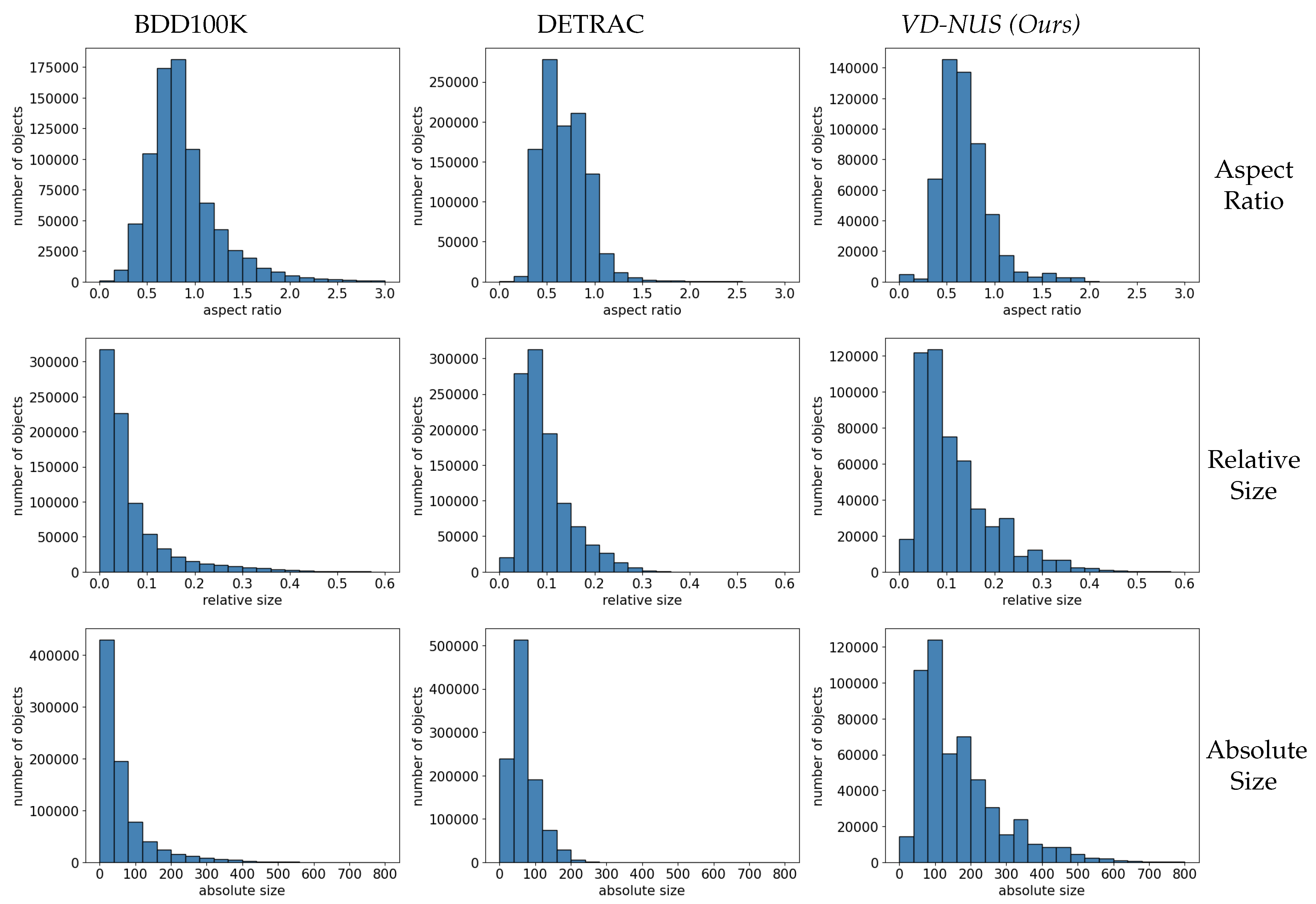
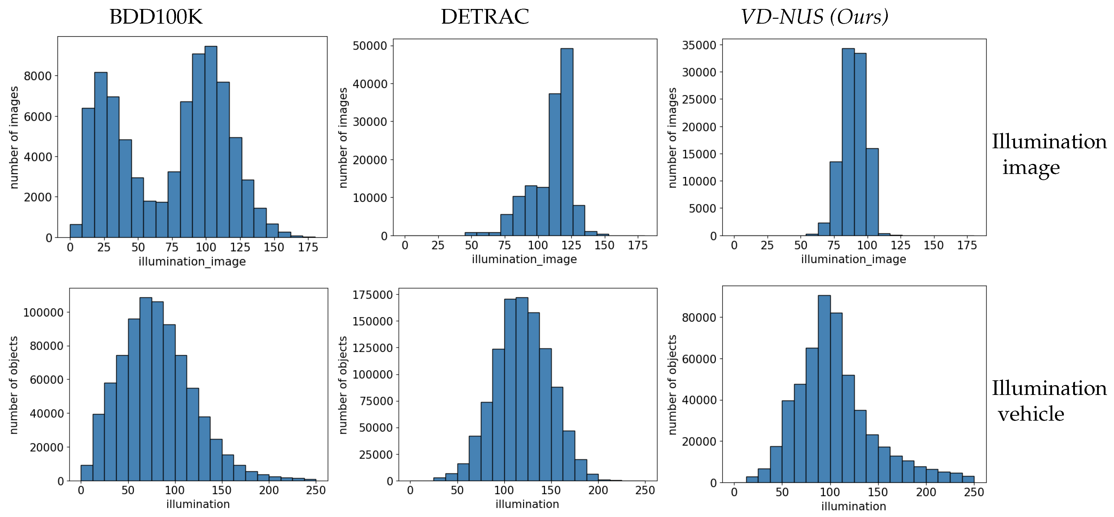
The characteristics are entirely different from existing datasets, such as scale (as shown in Figure 2) and illumination (as shown in Figure 3).
  • Scale. The camera has a long shooting distance in urban surveillance. Its scale is large when the vehicle is closer to the camera, while the scale is small when the vehicle is far from the camera. The diversity of different scales increases the difficulty of vehicle detection. The authors observed differences in several different scales of vehicles in BDD100K, DETRAC, and our VD-NUS datasets. In the case of aspect ratio and relative size, the distribution is relatively similar. However, the absolute size and the data distribution in our VD-NUS dataset are relatively diverse and rich.
  • Illumination. This paper examines the distribution of light in images and vehicles in several existing night-time datasets. Compared with the existing datasets, the VD-NUS dataset has a more concentrated distribution of light in the entire image and a more divergent distribution of light in the vehicles.

4. Active Auxiliary Mechanism for Vehicle Detection

Our goal is to train a robust vehicle detector with incomplete labeled samples in urban scenes. The detector can automatically build more annotation samples, alleviating the annotation workload when building the dataset. This study proposes a vehicle detection framework via AAM. The proposed AAM considers the localization instability and selects part of the training set, which contributes the most to the performance improvement in the detector. This section first introduces the overall framework of active learning for vehicle detection, and then describes how to select samples based on the uncertainty and robustness of the detector.

4.1. Overview

As shown in Figure 4, active learning is an iterative process of human–computer interaction. We initially collect a large number of unlabeled images S u from night-time urban scenes where active learning is applied to real-world scenes. In the first cycle, small portions of images are randomly selected from S U for manual labeling to construct the initial labeled set S L . Then, S L is used to train the detector for the initial detection model. After that, active learning enters an iterative process. Specifically, this process first relies on the meaningful information obtained by the detector to determine the next batch to be annotated. Secondly, this batch of images and their annotation information are updated to the set S A L after being manually annotated by the annotator. During the third step, S U is updated to S U S A L and S L is updated to S L S A L . Eventually, the updated annotated pool S L will be used as the training set to retrain the detector. The above process will be repeated until the detector performs satisfactorily.

4.2. Mixup

The challenge in active learning is how to effectively use the valid information from the model feedback in deciding the next training batch. In each round, the selected S A L according to the evaluation metric should have more information than S L , and the detector has not yet fully grasped this information. When the image is affected by noise such as illumination changes and occlusion, the detection result does not change drastically, indicating that the model already understands information in this part well enough. Therefore, these unlabeled images do not need to be labeled. In contrast, our method prefers to annotate images that show a dramatic change in detection results when some noise is added. To effectively filter out this type of image, AAM automatically selects images for human annotation depending on the image localization instability score ranking. Since several targets exist in the image, the sampling strategy requires first calculating the box scores in each image and then aggregating them to obtain per-image scores. Specifically, these scores are determined by both uncertainty and inconsistency. The former is defined by the confidence score within the detection result itself. The latter is estimated by comparing the inconsistency of the detection results between the original image and its augmented version.
Furthermore, a key factor that contributes to AAM choosing the data with the greatest improvement in detector performance via the consistency metric is robust data augmentation. This study adopts a series of data augmentation strategies for the images in S U , considering that vehicle detection at night is susceptible to noise such as imbalanced illumination, occlusion, and blurring. These include hue and saturation adjustments, horizontal flip, cutout, and Gaussian noise.
The current detection model was first used to obtain bounding boxes on the original image and the augmented image, respectively. The detection result of the original image is R b , c , where R b i , c i is the i-th prediction box. Each bounding box consists of localization information and classification information, where the former is defined by its central coordinates ( x , y ) , width w, and height h. In addition, augmentation operations were performed on each image in S U to obtain the set S U . Correspondingly, the detection results of the augmented image are R b , c , where R b i , c i is the i-th prediction box.
Before calculating the inconsistency of the prediction box, it is necessary to match the two detection results R b , c and R b , c . In this matching process, the detection boxes b i in R b , c will be matched one by one with each detection box b i in R b , c . B i will be chosen as the matching box for b i if the Intersection over Union ( I o U ) between B i and b i is maximal. The process can be described as follows:
B i = arg max b i b I o U ( b i , b i )
In particular, in Equation (1), this method additionally considers the situation where detection box b i does not have a matching detection box b i . Former inconsistency-based approaches simply and violently match detection frames, while not taking into account the false-positive boxes due to their own instability. If two detection boxes with no overlap are enforced to be matched, that instead disrupts the normal matching of the other detection boxes. Consequently, in this paper, the authors artificially provide a matching box for b i and set the IoU between them to 0.

4.3. Sample Selection

After the detection boxes are matched, I o U is directly used to assess whether the localization of the paired boxes is consistent. For any paired detection boxes b i and B i , their localization inconsistency is defined as follows:
L i n c o n f ( b i , B i ) = 1 I o U ( b i , B i )
Furthermore, our method not only consider the localization instability based on inconsistency, but also the uncertainty of detecting itself. Given a detection box R b i , c i , its uncertainty is defined as
U ( b i ) = 1 c i
Therefore, the final score of the detection box is
S ( b o x ) = L i n c o n f ( b i , B i ) + U ( b i )
In Equation (4), a higher S ( b o x ) for the detection box demonstrates that the detector has greater uncertainty, while it is also more easily influenced by noise. Accordingly, in theory, a higher box score implies that the corresponding region of the box is more informative. However, during the practical procedure, this study discovered that the boxes with extremely high scores are most likely to be noisy interference boxes. The reason behind this, as explained in this paper, is that even if the authors perform post-processing on the results (e.g., confidence filtering, non-maximum suppression), several background and redundant boxes are inevitably generated. Such boxes generally have rather low confidence scores to be high S ( b o x ) , which consequently misleads the data selection. This study should not simply conclude that a higher detection box score represents a more informative region, because this score would most probably be erroneously derived from the detector instability. On the other hand, a box approaching a score of 0 represents a high confidence level and an extremely well-matched overlap, which indicates a good understanding of this region. For this reason, the sampling strategy prefers to select detection boxes whose scores remain away from the minimum limit of 0, whilst also maintaining a reasonable distance from the maximum score of 2. Eventually, this method sets the detection box final score to
S ( b o x ) = min ( 1 , S ( b o x ) q )
The value of S’(box) is restricted to be between 0 and 1 by means of Equation (5), where the parameter q is determined empirically. The significance of the parameter q is that if the S ( b o x ) is around q, the information in the corresponding region is indeed not mastered by the detector. Finally, the minimum of all S’(box) in each image is taken as the score of that image, because the sampling strategy’s decision on whether an image is difficult or not is usually determined by some difficult objects and is not relevant to most simple objects.

5. Experiment

5.1. Datasets

This research validated the effectiveness of our active-learning-based method on the VD-NUS dataset (Figure 5). The VD-NUS comprises a total of 100,218 images, where the trainval set contains 70,160 images and the test set contains 30,058 images. We used the trainval set as the initial unlabeled set S U for our active learning process. In the evaluation phase, the active learning method was evaluated over VD-NUS’s test with the Average Precision ( A P ) [47] and log-average miss rate (MR−2) [48] metrics, where higher A P and lower MR−2 indicate better performance of the detection results.

5.2. Evaluation Metrics

AP. Before calculating the AP metric, precision and recall need to be obtained. The precision metric refers to the proportion of predictions that are truly correct compared to the predictions that the detector believes to be correct. Recall is the proportion of correctly detected objects to all ground truth. The two evaluation metrics, precision and recall, have been defined, respectively, as follows:
P r e c i s i o n = T P T P + F P
R e c a l l = T P T P + F N
In the above equation, true positive ( T P ) indicates the number of vehicles correctly detected, where both the detection result and the ground truth are vehicles. False positive ( F P ) means that the detector incorrectly considers the background as a vehicle, and false negative ( F N ) indicates the number of vehicles that the detector missed detecting. The A P summarizes the shape of the precision/recall curve, and is defined as the mean precision at a set of eleven equally spaced recall levels [0, 0.1, …, 1]:
A P = 1 11 r { 0 , 0.1 , , 1 } p interp ( r )
The precision at each recall level r is interpolated by taking the maximum precision measured for a method for which the corresponding recall exceeds r:
p interp ( r ) = max r ˜ : r ˜ r p ( r ˜ )
MR 2 . The evaluation metric is often used for pedestrian detection and reflects the false detection of the algorithm. This metric is obtained by quantizing the MR-FPPI curve, where the miss rate ( M R ) and false positive per image F P P I are, respectively, defined as follows:
M R = F N T P + F N
F P P I = F P N
The parameter N in Equation (11) is the number of images, so FPPI can obtain the average number of false positives per image.

5.3. Implementation Details

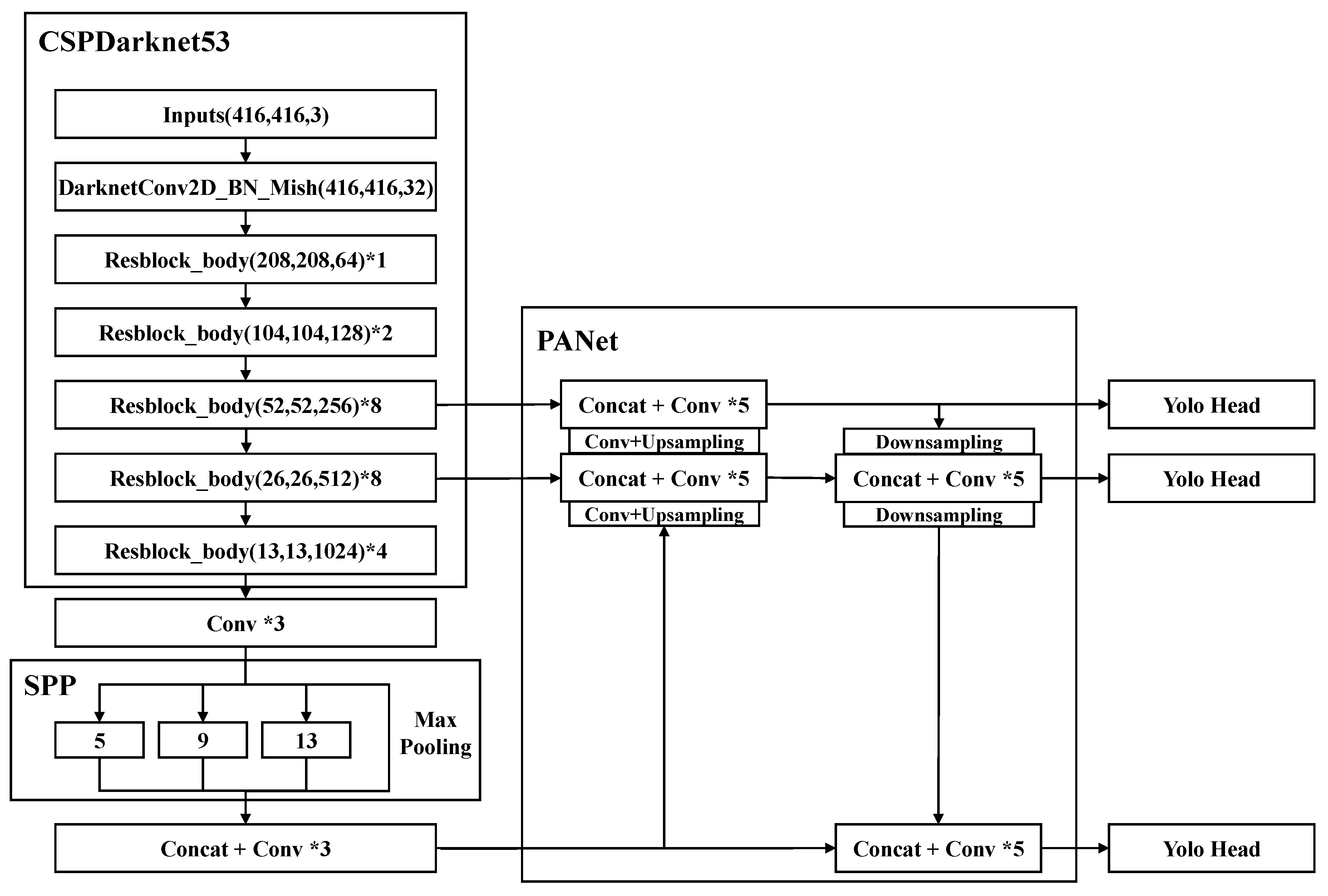
Single-stage detector YOLOv4 [49] was selected as our base object detector. As shown in the Figure 6, the backbone feature extraction network component, this detector chose CSPDarknet53 [50] as the backbone. YOLOv4 adds the SPP [51] module to separate out the most significant context features uses PANet as the method of parameter aggregation from different backbone levels for different detector levels. In each active learning cycle, this paper trains the model for 300 epochs and set the batch size to 8 in the initial 50 epochs during the freezing training stage and 4 in the latter 250 epochs of the unfreezing stage. In addition, in each cycle, the images in S L were re-divided into a training set and a validation set in a ratio of 9:1 for the model training. The model is initialized with weights trained on the COCO 2017 [52] training set. For VD-NUS, 1000 images were randomly selected from its training set as the initial labeled set S L . This work performed altogether 6 iterations of active learning, where 1000 images are selected from the remaining training set into S L in each active cycle.

5.4. Comparison with the State-of-the-Art Detection Models

To demonstrate the effectiveness of our method, random sampling was used as the baseline whilst comparing against other active-learning-based SOTA methods, including Learning Loss [42], LS+C [44] and CALD [54]. For the task-agnostic Learning Loss approach, this experiment introduced the loss prediction module and utilized the three feature layers output from the PANet part of the YOLOv4 model as a multi-layer feature to input into the loss prediction module for data selection and model training. For the CALD approach, only the first stage of the method was applied in the experimental setup. The detection results on the VD-NUS are shown in Figure 5, where our approach consistently achieves optimal performance in almost all active learning cycles, demonstrating the effectiveness of the proposed sampling strategy. In particular, AAM results in a 1% to 3% reduction in MR−2 in each active learning cycle compared to the random sampling strategy. For the metric AP, our approach outperforms random sampling by 0.91% and 0.49% when using 2000 and 3000 images, respectively.
This demonstrates the effectiveness of the method on the VD-NUS dataset, which is able to efficiently choose difficult samples through the uncertainty and localization instability of the detection results. Moreover, the overall trend shows that the performance of the respective approaches varies considerably in the early stages of iterative training, and gradually converges in the later cycles. This is due to the fact that with the increase in active learning iterations, the training data contain less knowledge that has not yet been learned by the detector. For the task-agnostic active learning method Learning Loss, it performed the worst, and even significantly lower than random sampling. The reason is that this type of method does not consider the characteristics of the localization for the object detection task. Therefore, the sample selected by this approach contains less knowledge that the detector has not yet mastered, whereas random selection at least ensures uniform sampling.

5.5. Discussion and Analysis

Scoring aggregating functions. This part of the experiment compares the active learning performance under different approaches to aggregating the bounding box scores S ( b o x ) into an image score. In order to verify whether it is reasonable to choose the minimum score of all detection boxes in each image as the image score, we also conducted an ablation study by averaging the scores of all detection boxes as image scores. The comparison of the experimental results between the two aggregation methods is shown in Table 2, where the performance of the detector degrades during the active learning iterations when the aggregation function changes from ’minimum’ to ’average’. The experimental results illustrate that whether an image is challenging or not has no relevance to the larger number of simple samples in the image, but depends on the few difficult objects.
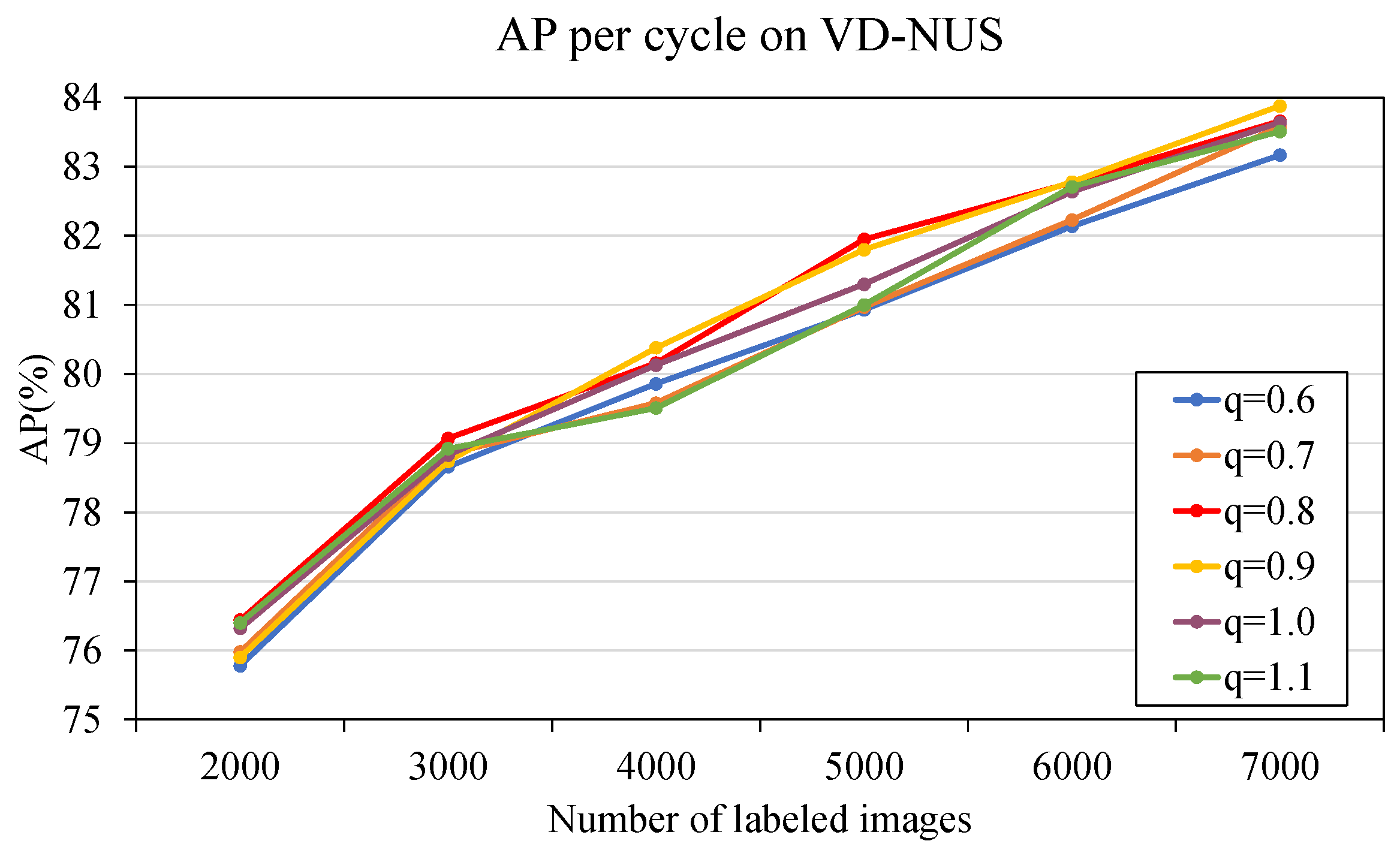
Optimum threshold q. S(box) in Equation (4) was directly applied as the final score of the bounding box to verify the reasonableness for the existence of q in Equation (5). As shown in Table 2, there is an overall significant drop in detection performance after the parameter q is removed. This experiment demonstrates that q can filter out some noise samples from the detection results. The optimal parameter q requires further confirmation. To this end, we conducted a series of experiments by taking the middle value 1 for q and then increasing or decreasing the value of q in 0.1 intervals in turn. The experimental results are shown in Figure 7. The performance drops slightly as q increases from 1.0 to 1.1, so the experimental setup did not continuously improve the value of q. In the process where q is varied from 1.0 to 0.6, it can be observed that the optimal performance is achieved by the experiment when q is set to 0.8. As q decreases further, the performance of the detector decreases. The reason for this is that the optimal value of S(box) will approach 0; consequently, the active learning selects samples that the detector has already mastered. On the other hand, when q is constantly rising, the detection box information becomes unstable, which also causes performance degradation.
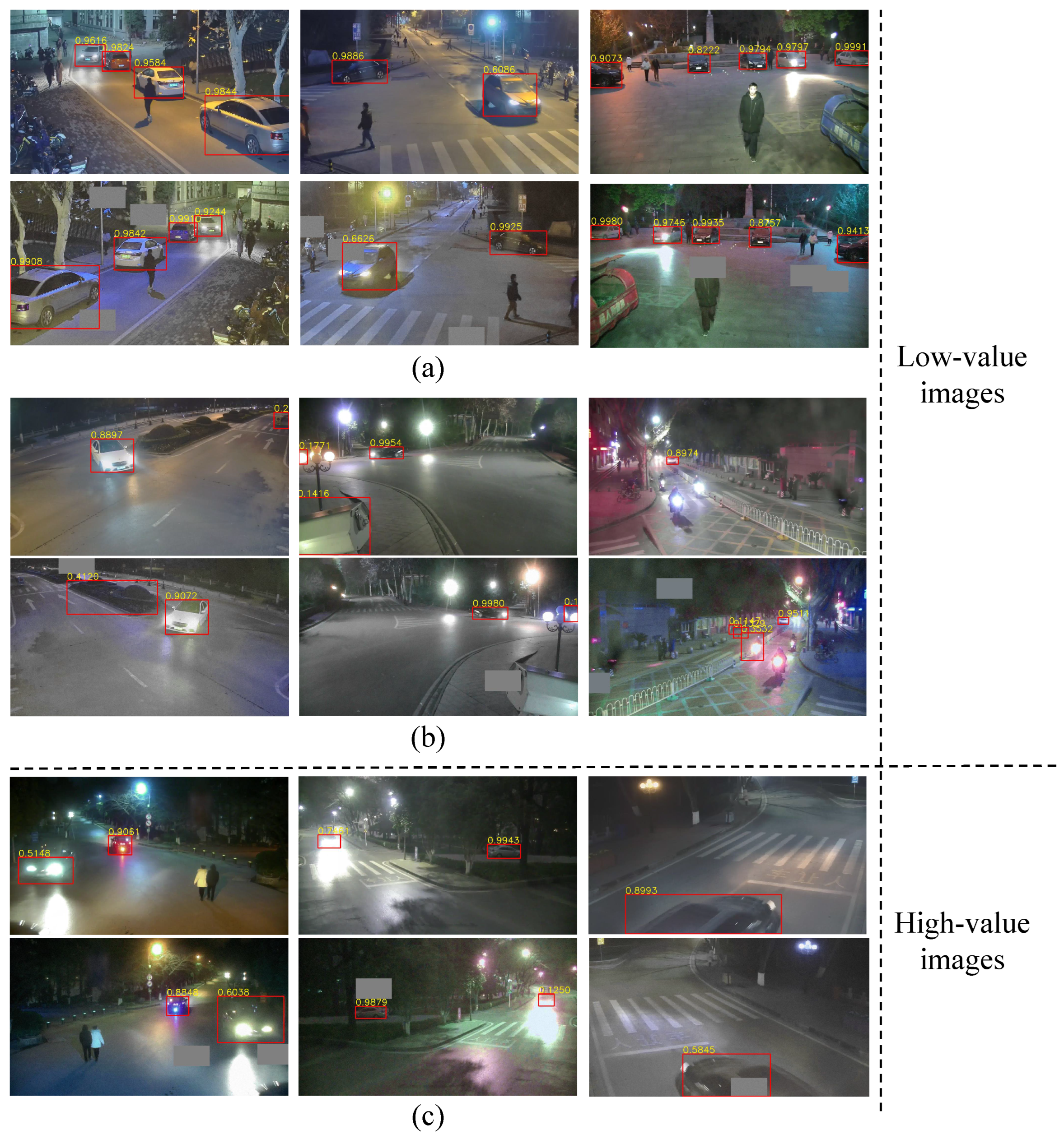
Representative examples of images with different scores are presented in Figure 8. For (a), the detector performs well enough on the image, which indicates that this image is unable to provide the detector with any more new information. It can be observed that the vehicles within the two pairs of images in situation (b) are correctly detected by the detector, but at the same time, many false-positive predictions are produced. Without q to constrain the false-positive boxes, the image score is dominated by the noise in the image background. In situation (c), the vehicle suffers from various degrees of exposure, occlusion, blurriness, etc., and the corresponding detection results are extremely unstable. These images with relatively reliable but unstable detection results are the ones that our sampling strategy favors.
Detector scalability. This method is not only applicable to one-stage object detectors. Therefore, the scalability of the approach was validated on the two-stage network Faster R-CNN [55] with Resnet-50 [56]. Likewise, random sampling was utilized as the baseline to validate whether our approach remains effective on the two-stage network. The experimental results are presented in Table 3. As shown in Table 3, our method outperforms the random sampling strategy, whether based on the one-stage object detector or the two-stage object detector. Particularly, based on the Faster R-CNN, our approach improves the detection performance AP by 0.53% and 0.96%, respectively, compared to random sampling when the number of annotated images is 3000 and 4000. For the M R 2 metric, A A M can improve performance by up to 3% compared to random sampling. In conclusion, our approach can be extended to other object detection networks.

6. Conclusions

In this paper, the authors present the first vehicle detection dataset collected from urban surveillance scenes, named VD-NUS, which exhibits a large number of vehicles from a variety of viewpoints. Capturing images from video to construct a dataset inevitably generates data redundancy. To address this challenge, this paper proposed a vehicle detection framework through AAM, which can train an effective vehicle detector with minimal labeled data. The proposed AAM framework can actively select informative images for annotation by estimating the localization instability of the detection results, consequently reducing the annotation workload and selecting informative samples. Additionally, this paper proposed a computer-assisted detection module embedded in the AAM framework to help annotators quickly and accurately label data. The experimental results demonstrate the effectiveness of our approach on the VD-NUS dataset.

6.1. Limitations

Although the uncertainty and localization instability scoring rules provided by the sampling strategy have achieved positive results and reduced the annotation workload when there is redundancy in the data, they did not take into account the diversity of the data when no redundancy exists. In future work, we will continue this study by further considering the diversity of the distribution of the data in the sampled set. On the other hand, the proposed VD-NUS dataset aims to compensate for the absence of a night-time vehicle detection dataset in urban surveillance scenes. Night-time vehicle detection in this scene has not been further investigated, so how to address such challenges as severe vehicle occlusion, richer viewpoints, and uneven illumination in this scene remains our future research direction as well.

6.2. Prospects

To explore the reason that the performance of these detectors is unsatisfactory on the VD-NUS dataset, further exploration is important. There are several challenges to night-time vehicle detection, such as light, scale, occlusion, and blur.
  • Light. The biggest difference between a night scene and a day scene is the absence of natural light. Night-time light sources mainly come from streetlights and vehicle headlights on the roadside. There is often low light when the vehicle is stopped. Exposure often exists when the vehicle is in motion. Enhancement of low light and suppression of exposure are important topics that favor vehicle detection at night.
  • Scale. Vehicles often traverse the entire frame when moving. They are easy to find when they are closer to the camera; however, they can be missed when they are farther away from the camera. Vehicles farther away from the camera are small in scale. The optimization of super-resolution or detection methods for small-scale vehicles at night is intuitively important for night-time vehicle detection research.
  • Occlusion. On peak congested roads, vehicles are closer to each other. It is difficult to see the full outline of the vehicle from the camera’s point of view, resulting in severe occlusion. This situation can bring about serious performance degradation. Completing the occluded area with information about the visible area of the vehicle can solve this problem to some extent.
  • Blur. The surveillance camera’s recording is uninterrupted, including at day and night. Due to long-term recording, equipment easily ages, and as a result this affects the camera imaging quality. The large temperature difference between day and night leads to increased fog, leading to seriously blurred images. On the other hand, the quality of images also reduces when images are sampled from the second night of surveillance due to the lower light. The current methods cannot be directly applied to practice, and the corresponding optimization techniques are needed to overcome the above problems.

Author Contributions

Validation, X.X.; Investigation, B.A.-H.; Resources, X.T.; Data curation, X.W.; Writing—original draft, X.W. and X.T.; Writing—review & editing, C.-W.L. All authors have read and agreed to the published version of the manuscript.

Funding

This work is supported by National Nature Science Foundation of China (62302351, 62376201), Nature Science Foundation of Hubei Province (2022CFB018), and Hubei Province Key Laboratory of Intelligent Information Processing and Real-time Industrial System (Wuhan University of Science and Technology) (ZNXX2022001).

Data Availability Statement

Data will be made available on request.

Conflicts of Interest

The authors declare no conflict of interest.

References

  1. Deng, Z.; Weng, D.; Liu, S.; Tian, Y.; Xu, M.; Wu, Y. A survey of urban visual analytics: Advances and future directions. Comput. Vis. Media 2023, 9, 3–39. [Google Scholar] [CrossRef] [PubMed]
  2. Xiao, J.; Wang, X.; Liao, L.; Satoh, S.; Lin, C.W. 1ST International Workshop on Visual Tasks and Challenges under Low-quality Multimedia Data. In Proceedings of the MMAsia ’21: ACM Multimedia Asia, Gold Coast, Australia, 1–3 December 2021; p. 1. [Google Scholar]
  3. Neumann, L.; Karg, M.; Zhang, S.; Scharfenberger, C. NightOwls: A Pedestrians at Night Dataset. In Proceedings of the Asian Conference on Computer Vision, Perth, Australia, 2–6 December 2018; pp. 691–705. [Google Scholar]
  4. Liu, P.; Fu, H.; Ma, H. An end-to-end convolutional network for joint detecting and denoising adversarial perturbations in vehicle classification. Comput. Vis. Media 2021, 7, 217–227. [Google Scholar] [CrossRef]
  5. Geiger, A.; Lenz, P.; Stiller, C.; Urtasun, R. Vision meets robotics: The KITTI dataset. Int. J. Robot. Res. 2013, 32, 1231–1237. [Google Scholar] [CrossRef]
  6. Yu, F.; Chen, H.; Wang, X.; Xian, W.; Chen, Y.; Liu, F.; Madhavan, V.; Darrell, T. BDD100K: A Diverse Driving Dataset for Heterogeneous Multitask Learning. In Proceedings of the Computer Vision and Pattern Recognition, Seattle, WA, USA, 13–19 June 2020; pp. 2633–2642. [Google Scholar]
  7. Wen, L.; Du, D.; Cai, Z.; Lei, Z.; Chang, M.; Qi, H.; Lim, J.; Yang, M.; Lyu, S. UA-DETRAC: A new benchmark and protocol for multi-object detection and tracking. Comput. Vis. Image Underst. 2020, 193, 1–27. [Google Scholar] [CrossRef]
  8. Wu, Z.; Xu, J.; Wang, Y.; Sun, F.; Tan, M.; Weise, T. Hierarchical fusion and divergent activation based weakly supervised learning for object detection from remote sensing images. Inf. Fusion 2022, 80, 23–43. [Google Scholar] [CrossRef]
  9. ElTantawy, A.; Shehata, M.S. Local null space pursuit for real-time moving object detection in aerial surveillance. Signal Image Video Process 2020, 14, 87–95. [Google Scholar] [CrossRef]
  10. Mou, Q.; Wei, L.; Wang, C.; Luo, D.; He, S.; Zhang, J.; Xu, H.; Luo, C.; Gao, C. Unsupervised domain-adaptive scene-specific pedestrian detection for static video surveillance. Pattern Recognit. 2021, 118, 108038. [Google Scholar] [CrossRef]
  11. Toprak, T.; Belenlioglu, B.; Aydin, B.; Güzelis, C.; Selver, M.A. Conditional Weighted Ensemble of Transferred Models for Camera Based Onboard Pedestrian Detection in Railway Driver Support Systems. IEEE Trans. Veh. Technol. 2020, 69, 5041–5054. [Google Scholar] [CrossRef]
  12. Chen, L.; Lin, S.; Lu, X.; Cao, D.; Wu, H.; Guo, C.; Liu, C.; Wang, F. Deep Neural Network Based Vehicle and Pedestrian Detection for Autonomous Driving: A Survey. IEEE Trans. Intell. Transp. Syst. 2021, 22, 3234–3246. [Google Scholar] [CrossRef]
  13. Yuan, T.; Wan, F.; Fu, M.; Liu, J.; Xu, S.; Ji, X.; Ye, Q. Multiple Instance Active Learning for Object Detection. In Proceedings of the Computer Vision and Pattern Recognition, Nashville, TN, USA, 20–25 June 2021; pp. 5330–5339. [Google Scholar]
  14. Xu, X.; Liu, L.; Zhang, X.; Guan, W.; Hu, R. Rethinking data collection for person re-identification: Active redundancy reduction. Pattern Recognit. 2021, 113, 107827. [Google Scholar] [CrossRef]
  15. Shahraki, A.; Abbasi, M.; Taherkordi, A.; Jurcut, A.D. Active Learning for Network Traffic Classification: A Technical Study. IEEE Trans. Cogn. Commun. Netw. 2022, 8, 422–439. [Google Scholar] [CrossRef]
  16. Zou, D.N.; Zhang, S.H.; Mu, T.J.; Zhang, M. A new dataset of dog breed images and a benchmark for fine-grained classification. Comput. Vis. Media 2020, 6, 477–487. [Google Scholar] [CrossRef]
  17. Zhang, W.; Guo, Z.; Zhi, R.; Wang, B. Deep Active Learning For Human Pose Estimation Via Consistency Weighted Core-Set Approach. In Proceedings of the International Conference on Image Processing, Anchorage, AK, USA, 19–22 September 2021; pp. 909–913. [Google Scholar]
  18. Deng, J.; Xie, X. 3D Interactive Segmentation With Semi-Implicit Representation and Active Learning. IEEE Trans. Image Process. 2021, 30, 9402–9417. [Google Scholar] [CrossRef]
  19. Leitloff, J.; Hinz, S.; Stilla, U. Vehicle Detection in Very High Resolution Satellite Images of City Areas. IEEE Trans. Geosci. Remote Sens. 2010, 48, 2795–2806. [Google Scholar] [CrossRef]
  20. Cao, L.; Ji, R.; Wang, C.; Li, J. Towards Domain Adaptive Vehicle Detection in Satellite Image by Supervised Super-Resolution Transfer. In Proceedings of the AAAI Conference on Artificial Intelligence, Phoenix, AZ, USA, 12–17 February 2016; pp. 1138–1144. [Google Scholar]
  21. Lyu, S.; Chang, M.C.; Du, D.; Wen, L.; Qi, H.; Li, Y.; Wei, Y.; Ke, L.; Hu, T.; Del Coco, M.; et al. UA-DETRAC 2017: Report of AVSS2017 & IWT4S Challenge on Advanced Traffic Monitoring. In Proceedings of the International Conference on Advanced Video and Signal Based Surveillance, Lecce, Italy, 29 August–1 September 2017; pp. 1–7. [Google Scholar]
  22. Lyu, S.; Chang, M.C.; Du, D.; Wen, L.; Qi, H.; Li, Y.; Wei, Y.; Ke, L.; Hu, T.; Del Coco, M.; et al. UA-DETRAC 2018: Report of AVSS2018 & IWT4S Challenge on Advanced Traffic Monitoring. In Proceedings of the International Conference on Advanced Video and Signal Based Surveillance, Auckland, New Zealand, 27–30 November 2018; pp. 1–6. [Google Scholar]
  23. Hu, X.; Xu, X.; Xiao, Y.; Chen, H.; He, S.; Qin, J.; Heng, P.A. SINet: A scale-insensitive convolutional neural network for fast vehicle detection. IEEE Trans. Intell. Transp. Syst. 2018, 20, 1010–1019. [Google Scholar] [CrossRef]
  24. Wang, H.; Yu, Y.; Cai, Y.; Chen, X.; Chen, L.; Liu, Q. A comparative study of state-of-the-art deep learning algorithms for vehicle detection. IEEE Intell. Transp. Syst. Mag. 2019, 11, 82–95. [Google Scholar] [CrossRef]
  25. Li, X.; Zhu, L.; Xue, Q.; Wang, D.; Zhang, Y.J. Fluid-inspired field representation for risk assessment in road scenes. Comput. Vis. Media 2020, 6, 401–415. [Google Scholar] [CrossRef]
  26. Shao, X.; Wei, C.; Shen, Y.; Wang, Z. Feature enhancement based on CycleGAN for nighttime vehicle detection. IEEE Access 2020, 9, 849–859. [Google Scholar] [CrossRef]
  27. Mu, Q.; Wang, X.; Wei, Y.; Li, Z. Low and non-uniform illumination color image enhancement using weighted guided image filtering. Comput. Vis. Media 2021, 7, 529–546. [Google Scholar] [CrossRef]
  28. Huang, S.; Hoang, Q.; Jaw, D. Self-Adaptive Feature Transformation Networks for Object Detection in low luminance Images. ACM Trans. Intell. Syst. Technol. 2022, 13, 13. [Google Scholar] [CrossRef]
  29. Liu, R.; Yuan, Z.; Liu, T. Learning TBox With a Cascaded Anchor-Free Network for Vehicle Detection. IEEE Trans. Intell. Transp. Syst. 2022, 23, 321–332. [Google Scholar] [CrossRef]
  30. Sivaraman, S.; Trivedi, M.M. Looking at Vehicles on the Road: A Survey of Vision-Based Vehicle Detection, Tracking, and Behavior Analysis. IEEE Trans. Intell. Transp. Syst. 2013, 14, 1773–1795. [Google Scholar] [CrossRef]
  31. Yin, G.; Yu, M.; Wang, M.; Hu, Y.; Zhang, Y. Research on highway vehicle detection based on faster R-CNN and domain adaptation. Appl. Intell. 2022, 52, 3483–3498. [Google Scholar] [CrossRef]
  32. Lyu, W.; Lin, Q.; Guo, L.; Wang, C.; Yang, Z.; Xu, W. Vehicle Detection Based on an Imporved Faster R-CNN Method. IEICE Trans. Fundam. Electron. Commun. Comput. Sci. 2021, 104-A, 587–590. [Google Scholar] [CrossRef]
  33. Vaquero, V.; del Pino, I.; Moreno-Noguer, F.; Solà, J.; Sanfeliu, A.; Andrade-Cetto, J. Dual-Branch CNNs for Vehicle Detection and Tracking on LiDAR Data. IEEE Trans. Intell. Transp. Syst. 2021, 22, 6942–6953. [Google Scholar] [CrossRef]
  34. Chadwick, S.; Newman, P. Radar as a Teacher: Weakly Supervised Vehicle Detection using Radar Labels. In Proceedings of the International Conference on Robotics and Automation, Paris, France, 31 May–31 August 2020; pp. 222–228. [Google Scholar]
  35. Waltner, G.; Opitz, M.; Krispel, G.; Possegger, H.; Bischof, H. Semi-supervised Detector Training with Prototypes for Vehicle Detection. In Proceedings of the Intelligent Transportation Systems Conference, Auckland, New Zealand, 27–30 October 2019; pp. 4261–4266. [Google Scholar]
  36. Feng, R.; Lin, D.; Chen, K.; Lin, Y.; Liu, C. Improving Deep Learning by Incorporating Semi-automatic Moving Object Annotation and Filtering for Vision-based Vehicle Detection. In Proceedings of the International Conference on Systems, Man and Cybernetics, Bari, Italy, 6–9 October 2019; pp. 2484–2489. [Google Scholar]
  37. Li, Y.; Wu, J.; Bai, X.; Yang, X.; Tan, X.; Li, G.; Wen, S.; Zhang, H.; Ding, E. Multi-Granularity Tracking with Modularlized Components for Unsupervised Vehicles Anomaly Detection. In Proceedings of the Computer Vision and Pattern Recognition, Seattle, WA, USA, 13–19 June 2020; pp. 2501–2510. [Google Scholar]
  38. Khorramshahi, P.; Peri, N.; Kumar, A.; Shah, A.; Chellappa, R. Attention Driven Vehicle Re-identification and Unsupervised Anomaly Detection for Traffic Understanding. In Proceedings of the Computer Vision and Pattern Recognition Workshops, Long Beach, CA, USA, 16–20 June 2019; pp. 239–246. [Google Scholar]
  39. Brust, C.A.; Käding, C.; Denzler, J. Active learning for deep object detection. arXiv 2018, arXiv:1809.09875. [Google Scholar]
  40. Elezi, I.; Yu, Z.; Anandkumar, A.; Leal-Taixe, L.; Alvarez, J.M. Not all labels are equal: Rationalizing the labeling costs for training object detection. In Proceedings of the Computer Vision and Pattern Recognition, New Orleans, LA, USA, 18–24 June 2022; pp. 14492–14501. [Google Scholar]
  41. Sener, O.; Savarese, S. Active learning for convolutional neural networks: A core-set approach. arXiv 2017, arXiv:1708.00489. [Google Scholar]
  42. Yoo, D.; Kweon, I.S. Learning loss for active learning. In Proceedings of the Computer Vision and Pattern Recognition, Long Beach, CA, USA, 16–20 June 2019; pp. 93–102. [Google Scholar]
  43. Choi, J.; Elezi, I.; Lee, H.J.; Farabet, C.; Alvarez, J.M. Active learning for deep object detection via probabilistic modeling. In Proceedings of the International Conference on Computer Vision, Montreal, BC, Canada, 11–17 October 2021; pp. 10264–10273. [Google Scholar]
  44. Kao, C.C.; Lee, T.Y.; Sen, P.; Liu, M.Y. Localization-aware active learning for object detection. In Proceedings of the Computer Vision–ACCV 2018: 14th Asian Conference on Computer Vision, Perth, Australia, 2–6 December 2018; Revised Selected Papers, Part VI 14, 2019. pp. 506–522. [Google Scholar]
  45. Ge, Z.; Liu, S.; Wang, F.; Li, Z.; Sun, J. YOLOX: Exceeding YOLO Series in 2021. arXiv 2021, arXiv:2107.08430. [Google Scholar]
  46. Chun, S.; Kim, W.; Park, S.; Chang, M.; Oh, S.J. Correcting False Negatives by Collecting Machine-and-Human-verified Image-Caption Associations for MS-COCO. In Proceedings of the European Conference on Computer Vision, Glasgow, UK, 23–27 October 2022; Volume 13668, pp. 1–19. [Google Scholar]
  47. Geiger, A.; Lenz, P.; Urtasun, R. Are we ready for autonomous driving? The kitti vision benchmark suite. In Proceedings of the 2012 IEEE Conference on Computer Vision and Pattern Recognition, Providence, RI, USA, 16–21 June 2012; pp. 3354–3361. [Google Scholar]
  48. Dollar, P.; Wojek, C.; Schiele, B.; Perona, P. Pedestrian detection: An evaluation of the state of the art. IEEE Trans. Pattern Anal. Mach. Intell. 2011, 34, 743–761. [Google Scholar] [CrossRef]
  49. Bochkovskiy, A.; Wang, C.Y.; Liao, H.Y.M. Yolov4: Optimal speed and accuracy of object detection. arXiv 2020, arXiv:2004.10934. [Google Scholar]
  50. Wang, C.Y.; Liao, H.Y.M.; Wu, Y.H.; Chen, P.Y.; Hsieh, J.W.; Yeh, I.H. CSPNet: A new backbone that can enhance learning capability of CNN. In Proceedings of the IEEE/CVF Conference on Computer Vision and Pattern Recognition Workshops, Seattle, WA, USA, 14–19 June 2020; pp. 390–391. [Google Scholar]
  51. He, K.; Zhang, X.; Ren, S.; Sun, J. Spatial pyramid pooling in deep convolutional networks for visual recognition. IEEE Trans. Pattern Anal. Mach. Intell. 2015, 37, 1904–1916. [Google Scholar] [CrossRef] [PubMed]
  52. Lin, T.Y.; Maire, M.; Belongie, S.; Hays, J.; Perona, P.; Ramanan, D.; Dollár, P.; Zitnick, C.L. Microsoft coco: Common objects in context. In Proceedings of the European Conference Computer Vision, Zurich, Switzerland, 6–12 September 2014; pp. 740–755. [Google Scholar]
  53. Redmon, J.; Farhadi, A. Yolov3: An incremental improvement. arXiv 2018, arXiv:1804.02767. [Google Scholar]
  54. Yu, W.; Zhu, S.; Yang, T.; Chen, C. Consistency-based active learning for object detection. In Proceedings of the Computer Vision and Pattern Recognition, New Orleans, LA, USA, 18–24 June 2022; pp. 3951–3960. [Google Scholar]
  55. Ren, S.; He, K.; Girshick, R.; Sun, J. Faster r-cnn: Towards real-time object detection with region proposal networks. Adv. Neural Inf. Process. Syst. 2015, 28, 1497. [Google Scholar] [CrossRef] [PubMed]
  56. He, K.; Zhang, X.; Ren, S.; Sun, J. Deep residual learning for image recognition. In Proceedings of the Computer Vision and Pattern Recognition, Las Vegas, NV, USA, 26 June–1 July 2016; pp. 770–778. [Google Scholar]
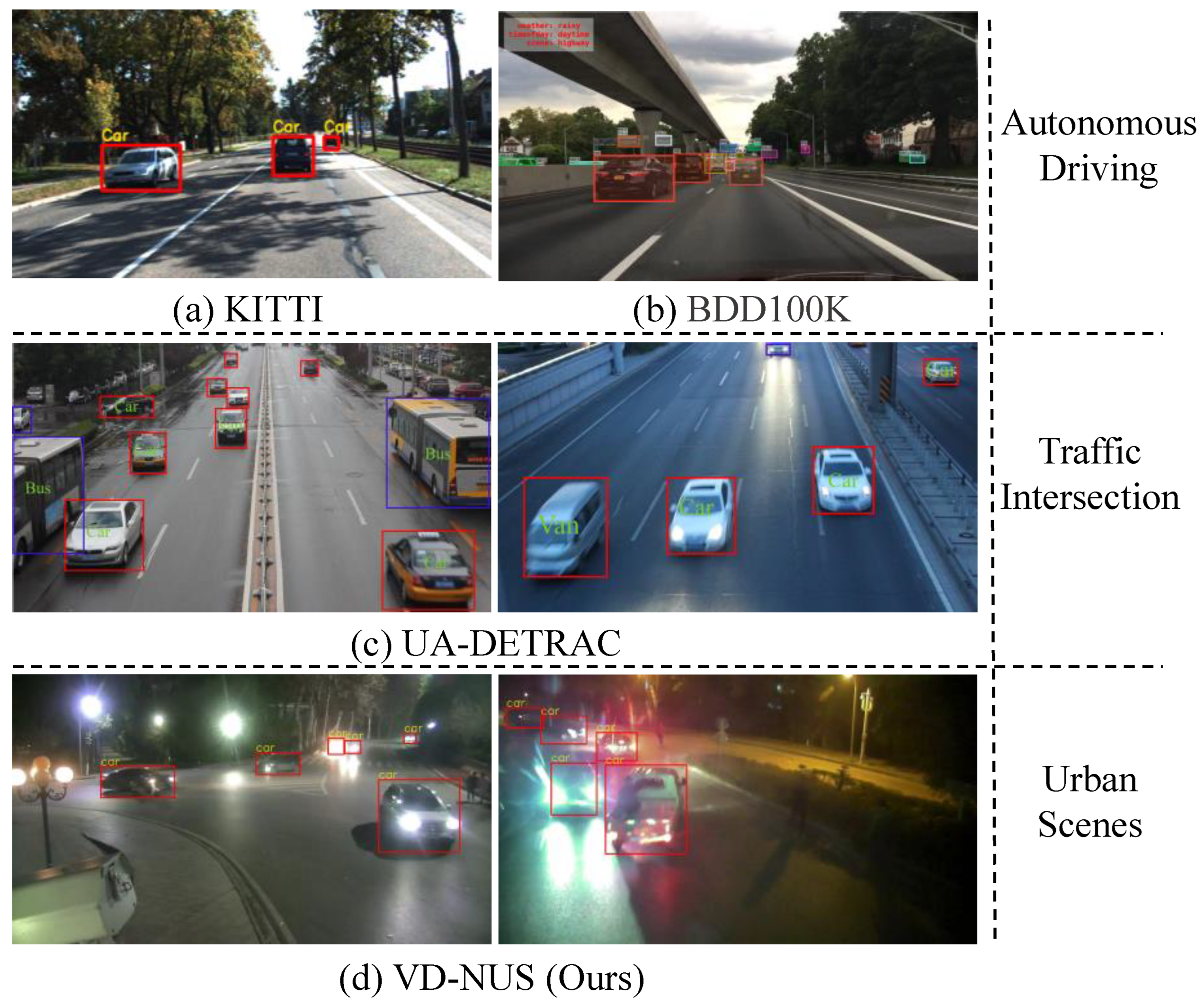
Figure 1. Comparison of the existing datasets and our dataset. (ad) exhibit samples from KITTI, BDD100K, UA-DETRAC, and our VD-NUS datasets, respectively. The scenes are shown with related datasets.
Remotesensing 15 04310 g001
Figure 2. Comparison of the existing datasets and our dataset. The distribution of aspect ratio, relative size, and absolute size is exhibited from top to bottom.
Remotesensing 15 04310 g002
Figure 3. Comparison of the existing datasets and our dataset. The first and second rows exhibit the illumination distribution for the whole image and the vehicle section, respectively.
Remotesensing 15 04310 g003
Figure 4. The overall framework of AAM. In each active learning cycle, the sampling strategy scores each bounding box by considering the uncertainty within the detection result itself and the inconsistency between it and the augmented image detection result. These box-level scores are then aggregated into image scores, which are used to select images for annotation.
Remotesensing 15 04310 g004
Figure 5. Comparison with other state-of-the-art active learning methods on VD-NUS dataset. (Left) Log-average miss rate metric. (Right) Average Precision metric.
Remotesensing 15 04310 g005
Figure 6. The overall framework of the YOLOv4 detector, which includes CSPDarknet53 backbone, SPP additional module, PANet path-aggregation neck, and YOLOv3 [53] (anchor-based) head.
Remotesensing 15 04310 g006
Figure 7. Performance of the detector under different q parameter.
Remotesensing 15 04310 g007
Figure 8. Visualization of the detection results for original and augmented images: (a) Detector performs well on the image. (b) Image score is dominated by false-positive predictions. (c) Images that our active learning approach utilized.
Remotesensing 15 04310 g008
Table 1. Overall distribution of VD-NUS and existing vehicle detection datasets.
DatasetTrainValTestImagesizeScene
ImagesBoxes (Car)Night-Time ImagesImagesBoxes (Car)Night-Time ImagesImagesBoxes (Car)
KITTI748128,742----7518-1242 × 375Autonomous Driving
BDD100K70,000714,12128,028 (40.04%)10,000102,5403929 (39.29%)20,000205,2141280 × 720
UA-DETRAC83,791503,85322,819 (27.23%)---56,340548,555960 × 540Traffic Intersection
VD-NUS60,137305,22360,137 (100%)10,02351,29010,023 (100%)30,058153,1631920 × 1080Urban Scenes
Table 2. AP (%) by using different components of the AAM.
MethodInconsistency-Based ScoringqMinAverageNumber of Labeled Images
200030004000500060007000
Random 75.5378.5880.1281.4282.4683.46
Ours 75.9578.3480.2181.9282.7583.95
76.4479.0780.1681.9582.7783.66
72.8975.7577.3178.2579.1980.92
Table 3. Performance of our approach on VD-NUS based on different detectors.
ModelMethodNumber of Labeled ImagesMetric
RandomAAM1000200030004000500060007000
YOLOv4 68.2275.5378.5880.1281.4282.4683.46 A P
68.2276.4479.0780.1681.9582.7783.66
0.650.550.490.460.430.410.39 M R 2
0.650.520.460.440.410.400.37
Faster R-CNN 82.1883.9784.7684.9685.3985.5185.89 A P
82.1884.1785.2985.9285.8186.3886.06
0.40.370.360.360.350.350.33 M R 2
0.40.380.350.330.330.320.32
Disclaimer/Publisher’s Note: The statements, opinions and data contained in all publications are solely those of the individual author(s) and contributor(s) and not of MDPI and/or the editor(s). MDPI and/or the editor(s) disclaim responsibility for any injury to people or property resulting from any ideas, methods, instructions or products referred to in the content.