Article

A Random Forest Algorithm Combined with Bayesian Optimization for Atmospheric Duct Estimation

1
School of Science, Xi’an University of Posts and Telecommunications, Xi’an 710121, China
2
School of Physics, Xidian University, Xi’an 710071, China
*
Author to whom correspondence should be addressed.
Remote Sens. 2023, 15(17), 4296; https://doi.org/10.3390/rs15174296
Submission received: 15 June 2023 / Revised: 15 July 2023 / Accepted: 26 July 2023 / Published: 31 August 2023

Abstract

:
Inversion of atmospheric ducts is of great importance in the field of performance evaluation for radar and communication systems. Since the model parameters in machine learning play a crucial role in prediction performance, this paper develops a random forest (RF) model integrated with Bayesian optimization (BO) called BO-RF for atmospheric duct prediction, and the BO is adopted to determine appropriate model parameters during the training process. In addition, the K-fold cross-validation (CV) method is also incorporated into the model to obtain the best model partition and overcome the overfitting problem. To test the performance of the proposed model, the results obtained by the BO-RF are compared with other commonly used methods, such as classical RF, extreme gradient boosting (XGBoost) with/without BO, and K-nearest neighbor (KNN) with/without BO. Comparisons demonstrate that BO-RF has the best accuracy and anti-noise ability for the estimation of duct parameters.

1. Introduction

An atmospheric duct is an anomalous electromagnetic propagation phenomenon that commonly appears in the maritime environment and can have a significant impact on radar and communication systems, such as communication blind areas, increased radar sea surface clutter, etc. Therefore, accurate analysis of radar echoes and efficient estimation of atmospheric duct parameters have become active research fields. Atmospheric ducts generally consist of three types, including evaporation ducts, surface-based ducts (SBDs), and elevated ducts. Evaporation ducts and SBDs are two common types in maritime environments due to the rapid changes in vertical atmospheric and humidity profiles with altitude above the sea surface [1]. It should be noted that SBDs exhibit a lower probability of occurrence than evaporation ducts, but their influence on radar and communication systems is much greater than that of evaporation ducts.
Estimation of atmospheric duct refractivity parameters with the refractivity from clutter (RFC) technique has attracted considerable interest in the field of optimization theory. Numerous methods have been proposed to retrieve atmospheric refractivity parameters. Gerstoft et al. [2,3] published simulation results for an eleven-parameter refractivity profile with five parameters in the vertical direction and six parameters in the horizontal direction, solved using a genetic algorithm, and presented the key steps and the latest research progress regarding the RFC technique. Douvenot et al. [4] first employed the least squares support vector, which belongs to a class of machine learning based on the pregenerated radar sea clutter power (RSCP) database produced by the parabolic wave equation (PWE), to estimate SBD. Wang et al. [5] inverted the evaporation duct using particle swarm optimization with RFC. Zhang et al. [6] proposed a four-parameter evaporation duct model and retrieved refractivity parameters from it. Zhao et al. [7] applied classical simulated annealing to the remote sensing of an atmospheric duct. Yang et al. [8,9,10,11] performed the inversion of an atmospheric duct with standard and improved swarm intelligence optimization and presented a comparison of the machine learning algorithm for evaporation duct estimation. Tepecik et al. [12] introduced a novel hybrid model based on an artificial neural network and a genetic algorithm for the inversion problem of refractivity estimation. Lentini et al. [13] calculated the global sensitivity of radar wave propagation to environmental parameters at the maritime atmospheric boundary layer. Penton et al. [14] studied the influence of rough ocean surfaces on evaporation duct atmospheric refractivity inversion with a genetic algorithm. Pozderac et al. [15] adopted a novel transmit–receive array system named the X-band beacon-receiver array to determine the maritime evaporation duct. Yan et al. [16] proposed an estimation method for evaporation ducts using a neural network. Zhu et al. [17] predicted evaporation duct height based on a multilayer perceptron network. Sit et al. [18,19] showed that deep learning and artificial neural networks can be efficiently used to classify and predict atmospheric ducts. It is of great significance to obtain instantaneous environmental information for assessing the performance of radar and communication systems. It can be distinctly seen from the above study that more and more attention has been paid to the field of monitoring the atmospheric environment in the maritime boundary layer with machine learning due to its superiority in real-time compared with swarm intelligence optimization. Random forest (RF) [20,21] is a powerful machine learning algorithm inspired by the ensemble learning method that works by incorporating many decision trees into one algorithm model to enhance its performance. However, the hyper-parameter in RF that directly relates to the performance of machine learning is difficult to determine. In this paper, a combination of RF with Bayesian optimization (BO) is presented to predict atmospheric duct parameters, where BO is adopted to search for the most appropriate hyper-parameter during the training process. To test the performance of the proposed BO-RF model, the RSCP versus propagation distance is numerically simulated by the PWE method with the combinations of refractivity parameters generated with an orthogonal experiment design (OED) method; the results obtained by the BO-RF are compared with the commonly used methods, such as classical RF, extreme gradient boosting (XGBoost) [22] with/without BO, and K-nearest neighbor (KNN) [23] with/without BO. Comparisons demonstrate that BO-RF has the best accuracy and noise immunity for the estimation of atmospheric duct parameters.

2. Forward Model

The forward model commonly includes two parts: the refractivity model and the radar propagation model. In the subsequent section, we will introduce the basic concept in the field of atmospheric ducts.

2.1. Refractivity Model

As the radio wave travels in the electromagnetic duct, the propagation features of the radio wave are controlled by the index of refraction:
n = c / v ,
where c is the speed of light in a vacuum and v is the speed of light in the medium. The value of n is close to unity, typically 1.00035; however, even a tiny variation in the refractive index may cause a huge change in the propagation features. Hence, a useful dimensionless physical variable N , which is the part-per-million change in the index of refraction, named refractivity, is introduced:
N = ( n 1 ) × 10 6 .
To further account for the curvature of the earth, another variable M called modified refractivity is provided by
M ( z ) = N + z R e × 10 6 = N + 0.157 z ,
where R e is the radius of the earth and z is the height above the earth’s surface. As d M / d z < 0 , an electromagnetic duct that can confine radio wave propagation and act like a waveguide is formed [24,25]. In this paper, our emphasis is placed on the three parameters of SBD shown in Figure 1, according to [26].
M ( z ) = M ( 0 ) + { c 1 z z z b c 1 z b M d z - z b z t h i c k z b < z < z t h i c k c 1 z b M d + c 2 ( z z b z t h i c k ) z z t h i c k ,
where M ( 0 ) is the modified refractivity at the mean sea level, typically taken as 330   M - units , z describes the height from the mean sea level, z b and z t h i c k represent the thicknesses of the base layer and trapping layer, c 1 and c 2 denote the slopes of the base layer and top layer, and M d is the duct strength. Obviously, there are three parameters in the SBD refractivity profile model, and we will employ the parametrization refractivity model of SBD via M = ( z b , z t h i c k , M d ) . The tri-linear refractivity profile for SBD is shown in Figure 1.

2.2. PWE Method

PWE can be divided into a narrow-angle and a wide-angle PWE. The propagation elevation of the narrow-angle PWE has good accuracy when it does not exceed 15 ° . An atmospheric duct usually occurs when the trapping angle does not exceed 1 ° . Therefore, the narrow-angle PWE is selected for studying the radio wave for long-range propagation in atmospheric ducts [27]. In order to analyze the two-dimensional tropospheric propagation problem, the scalar wave equation taking the index of refraction n into account is provided by [28]:
2 φ x 2 + 2 φ z 2 + k 0 2 n 2 φ = 0 ,
where φ ( x , z ) represents the electric or magnetic field component, k 0 is the wavenumber in a vacuum, and x and z are the range and height, respectively. It is a good approximation if the index of refraction varies slowly with the propagation direction. With the help of the reduced function φ ( x , z ) = u ( x , z ) e i k 0 x and the paraxial approximation, the PWE is expressed by
2 u z 2 + 2 i k 0 u x + k 0 2 ( n 2 1 ) u = 0 .
Then, the split-step Fourier-transform solution to the PWE can be written as [29]
u ( x 0 + Δ x , z ) = e i k 0 M ( z ) 1 0 6 Δ x 1 { e i p 2 Δ x / 2 k 0 { u ( x 0 , z ) } } ,
where p is the transform variable, and and 1 denote the forward Fourier transform and inverse Fourier transform, respectively. If the initial field u ( x 0 , z ) is provided, the field distribution along the vertical direction at each range interval can be easily marched in a horizontal range.
Once the field distribution of the entire computational region is obtained with Equation (7), the RSCP can be easily expressed in dB at range x by radar theory [2],
P c ( x , M ) = 2 L ( x , M ) + 10   l o g ( x ) + σ ° + C 0 ,
where M is the parameterized vector of the atmospheric environment, σ ° is the normalized scattering coefficient from the sea surface, C 0 is a constant that contains the parameters of the radar system, and L ( x , M ) is the propagation loss in the atmospheric duct environment that can be conveniently computed from the field distribution.

3. Optimization Algorithm

3.1. Principle of RF Regression

Decision tree is the primary component of RF and belongs to a class of machine learning that generally includes three main steps: feature selection, decision tree generation, and pruning of the decision tree. RF commonly adopts the decision tree that has not completed the pruning optimization operation. Each decision tree makes a prediction for the sample, and the final prediction can be achieved by taking the average of the combined predictions of all decision trees [30]. It has strong robustness and flexibility in dealing with regression problems. However, it has the shortcomings of falling into the local optimum, leading to high complexity and overfitting.
RF is an integrated learning algorithm using decision tree modeling, consisting of multiple independent decision trees. Different decision trees are constructed from random samples, but there is no relationship between them, and the output of the model is determined by each decision tree. In the process of training decision trees, randomly selected features further improve the model’s accuracy and avoid insufficient generalization ability. The detailed steps are given as follows:
  • A bootstrap method is adopted to randomly selected M sample points from the original sample dataset S to construct a decision tree and its training subset.
  • The training subset is used to train each decision tree. Assume that the number of input features to the dataset is N . The split rule for each node is to randomly select k features from the N features as alternative branch features, and then select the best split node from the k features to divide the left and right subspaces. Each split node performs a binary test on each subset, and the test result is sent to the left or right sub-node. The test randomly chooses a subset of features and finds a value with the lowest mean square error κ to group and determine its optimal branch, and it can be expressed as
    κ = 1 D 1 i D 1 ( E i C 1 ) 2 + 1 D 2 i D 2 ( E i C 2 ) 2 ,
    where E i is the true value of the ith sample, and C 1 and C 2 are the sample predictions for the left and right subspaces D 1 and D 2 , respectively.
  • Multiple decision trees can be generated via the first two steps above. The final prediction of each decision tree depends on the average of the leaf nodes where the sample points are located. The accuracy of RF is further improved by optimizing parameters such as the number of decision trees, the maximum depth of the decision tree, the minimum number of samples required for node division, the minimum sample number of the leaf nodes, and the number of features in the tree.
  • Finally, a RF model is produced by taking the average of the multiple decision trees as follows:
    f ( x ) = 1 k i = 1 k E i ( x ) ,
    where f ( x ) denotes the combined regression model.

3.2. BO Algorithm

BO is a novel and efficient hyper-parameter tuning algorithm [31,32]. In BO, the objective function distribution is first evaluated by Bayes’ theorem, and the new hyper-parameter for the algorithm are then selected according to the optimal sampling point distribution of the objective function. In addition, the update of the hyper-parameter for the next time depends on the objective function value of the optimal sample point. BO is mainly composed of the probabilistic proxy model and the acquisition function. In the following, we will briefly introduce the two parts.

3.2.1. Probabilistic Proxy Model

The updated formula in the probabilistic proxy model is given by
p ( f | D 1 : t ) = p ( D 1 : t | f ) p ( f ) p ( D 1 : t ) ,
where f represents the objective function, D 1 : t = { ( x 1 , f 1 ) , ( x 2 , f 2 ) , L ( x t , f t ) } denotes the collection of sampling point, p ( D 1 : t | f ) is the likelihood distribution of observation set, p ( f ) is the prior probability distribution of f , and p ( f | D 1 : t ) represents the posterior probability distribution of f and is used to modify and test the unknown target function.
The probabilistic proxy model can be divided into parametric and non-parametric models. The Gaussian process is a commonly adopted non-parametric model that has a strong ability to fit functions and is widely used in the field of regression.
A Gaussian process is entirely defined by the mean function m ( x ) and the covariance function K ( x , x ) as
f ( x ) ~ G P ( m ( x ) , K ( x , x ) ) ,
where the mean function is a vector and the covariance function is a matrix.
If we assume that there is a collection of sample points D = { ( x 1 : t , y 1 : t ) } , its covariance matrix is given by
K = [ k ( x 1 , x 1 ) k ( x 1 , x 2 ) k ( x 1 , x t ) k ( x 2 , x 1 ) k ( x 2 , x 2 ) k ( x 2 , x t ) k ( x t , x 1 ) k ( x t , x 2 ) k ( x t , x t ) ] .
When a set of sample ( x t + 1 , f t + 1 ) is added to the collection of historical evaluation points, supposing that k = [ k ( x t + 1 , x 1 ) k ( x t + 1 , x 2 ) k ( x t + 1 , x t ) ] , the corresponding covariance matrix can be updated by
K = [ K k T k k ( x t + 1 , x t + 1 ) ] .
Using the updated covariance matrix, the posterior probability distribution of f t + 1 is computed from the first t samples
{ p ( f t + 1 | D 1 : t , x t + 1 ) ~ N ( μ , δ 2 ) μ = k T K - 1 f 1 : t δ 2 = k ( x t + 1 , x t + 1 ) k T K - 1 k .

3.2.2. Acquisition Function

In the Gaussian process, the acquisition function is adopted to balance the ability of exploration and exploitation and search for the optimal objective function value for the next iteration to obtain the optimal hyper-parameter. Currently, the probability of improvement (PI), expected improvement (EI), and upper confidence bound (UCB) are widely used for acquisition functions. In this paper, PI is selected as the acquisition function, and it can be expressed as follows:
t ( x ; D 1 : t ) = p ( f ( x ) v * ξ ) = ϕ ( v * ξ μ t ( x ) δ t ( x ) ) ,
where v * represents the current optimal function value, ϕ ( ) is the cumulative density function of the standard normal distribution, and ξ is the balance parameter. The problem of local optimum can be overcome to a certain extent and the optimal value can be globally searched by adjusting the parameter ξ .

4. A Hybrid BO-RF Model

4.1. Orthogonal Experimental Design Method

In order to train the RF model, an OED method is used to generate the combinations of refractivity parameters. It is well known that OED is a robust way to effectively handle multi-dimension and multi-factor problems because it can select a few representative combinations in the experimental database to obtain the optimal result. The key in OED is the orthogonal array (OA) that can reflect the characteristics of each dimension. Thus, we first need to construct an appropriate OA. Here, we use L M ( Q N ) to represent an OA with N factors and Q levels per factor, where M is the number of combinations of levels. Then, we take a three-factor problem as an example by setting Q = 3 and N = 3 to obtain an orthogonal table L 9 ( 3 3 ) [33,34,35]:
L 9 ( 3 3 ) = [ 1 1 1 1 2 2 1 3 3 2 1 2 2 2 3 2 3 1 3 1 3 3 2 1 3 3 2 ] .
In L 9 ( 3 3 ) , there are three columns, showing that it is suitable for the problem with three parameters at most, and nine rows, demonstrating that one can do nine experiments for a combination with different levels. Each row in (17) represents an experiment with different levels. Normally, we should carry out 3 3 = 27 combinations of experiments for a three-factor and three-levels-per-factor problem. However, this task can be reduced to 3 2 = 9 combinations of experiments with the help of OA.
An orthogonal expansion is made based on OED. Assuming the lower and upper boundaries of a D-dimension parameter are u = ( u 1 , u 2 , u D ) and t = ( t 1 , t 2 , t D ) , the range of the corresponding cross-solutions are determined by
l o w = ( min ( u 1 , t 1 ) , min ( u 2 , t 2 ) , min ( u D , t D ) ) ,
u p = ( max ( u 1 , t 1 ) , max ( u 2 , t 2 ) , max ( u D , t D ) ) .
In the cross-solution, the range of the ith dimension variable x i is [ l o w i , u p i ] = [ min ( u i , t i ) , max ( u i , t i ) ] . The ith dimension variable x i can be quantized into Q levels according to the following formula:
l i , j = { l o w i j = 1 l o w i + j 1 Q 1 ( u p i l o w i ) 2 j Q 1 u p i j = Q .
Then, we use L M ( Q N ) to construct M feasible combinations. More detailed information can be found in [33,34,35].
The inversion of SBD is a three-parameter problem, and the lower and upper boundaries are given by t = ( 0 , 20 , 20 ) and u = ( 100 , 100 , 100 ) , respectively [4]. Let us first construct an appropriate OA L M ( Q N ) with Q = 100 , N = 3 , and M = 10,000 for the purpose of generating 10,000 training datasets [4].

4.2. Range of the Hyper-Parameter in RF

The hyper-parameter in RF mainly includes the number of decision trees, maximum depth, minimum samples of split, minimum samples of leaf, and maximum features in the tree. The range of hyper-parameter is shown in Table 1.

4.3. BO-RF Model

The core of the RF model lies in the selection of the hyper-parameter. In this paper, a BO-RF is adopted to predict the refractivity parameter of an atmospheric duct, and the BO is incorporated into the RF to find the best hyper-parameter. In addition, we apply K-fold cross-validation (CV) technology [36] to the BO-RF, which is commonly used to evaluate the training effect and avoid overfitting phenomenon. The CV makes full use of limited data, and the evaluation results may be as close as possible to the performance of the model on the test set, which can be used as an indicator for model optimization.
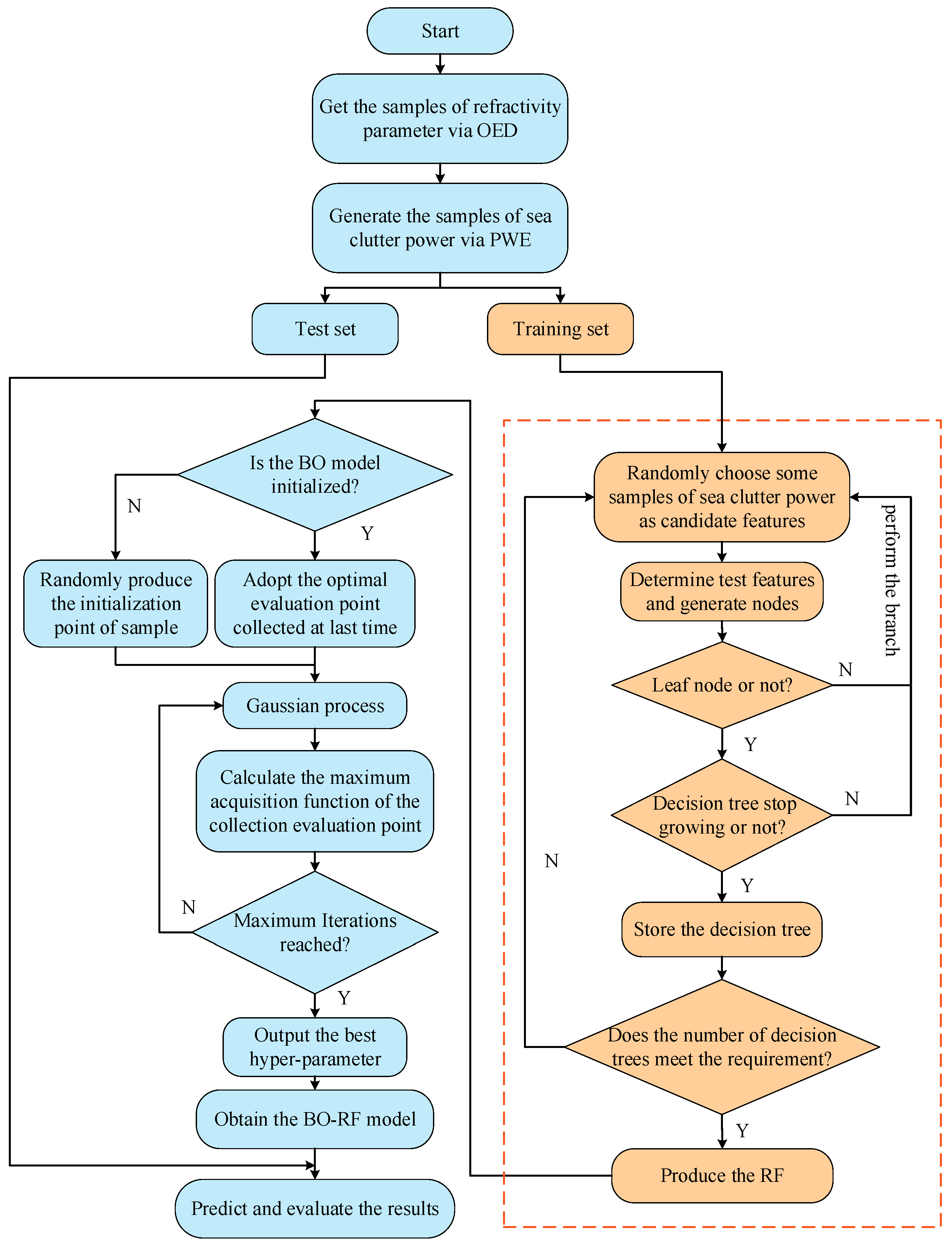
In BO-RF, the input and output datasets are first used to train the RF model and optimize the RF parameters. Then, the probabilistic proxy model for the estimation of atmospheric duct is constructed and optimized to obtain the best hyper-parameter in RF. Up to this point, the BO-RF model has been successfully established. The flowchart of the BO-RF is shown in Figure 2 for atmospheric duct estimation. The corresponding optimization process is given as follows:
  • An OED method is used to generate the combinations of refractivity parameters.
  • The split-step Fourier-transform solution to the PWE is adopted to generate the RSCP samples according to the combinations of refractivity parameters.
  • A bootstrap method is used to produce decision trees from the training set and then form a random forest.
  • A group of hyper-parameter is randomly selected within the scope of the parameter to produce the corresponding initialization point of the sample, then substituted into the RF model to obtain the corresponding objective function f and the initial sample set D .
  • The probabilistic proxy model in BO is applied to fit ( x , f ) and find the most possible evaluation point x t in the sample, which can be used to obtain the optimal acquisition function. Furthermore, the hyper-parameter is then assigned to RF model to find the objective function value f t of the optimal sample point and use it as the basis for selecting the hyper-parameter next time.
  • A new set of sampling points ( x t , f t ) is added to the historical sample set D t - 1 , and the Gaussian process is adjusted to optimize the objective function in it.
  • The BO stops updating as soon as it reaches the maximum number of iterations. That is to say, the best hyper-parameter, the optimal value of the objective function, and the corresponding BO-RF model are determined.
  • The test set is then used to examine the BO-RF model.
  • The results are evaluated and analyzed.

5. Results and Discussion

5.1. Simulations of the RSCP in SBD

In this section, the RSCP versus propagation distance are numerically simulated by Equation (8) via the PWE method. In order to estimate the refractivity profile with the RFC technique, the RSCP should be sensitive to the refractivity parameters of SBD. In the simulations, the radar system parameters are given in Table 2, and the parameterized vector of refractivity profile for SBD is M = ( 30 , 42 , 71 ) .
Firstly, the curve of RSCP versus the propagation distance at different receive heights are shown in Figure 3. It can be clearly seen that the RSCP in SBD is distinctly sensitive to the receive height.
Furthermore, the coverage diagrams are presented in Figure 4, Figure 5 and Figure 6 to examine the change in RSCP in SBD with every dimension of the parameterized vector. It is obvious that the spatial distributions of RSCP change as each parameter in refractivity profile changes. In other words, the spatial distributions of RSCP vary obviously with the parameters in SBD.

5.2. Estimation of SBD

To test the performance of the BO-RF, the estimation study of three parameters SBD with RFC is carried out, and the results obtained by the BO-RF are compared with the results obtained from commonly used methods, such as classical RF, XGBoost with/without BO, and KNN with/without BO. The radar system parameters are identical to those given in Table 2. In order to fully consider the propagation characteristics of the SBD and reduce the number of training samples, the OED method is adopted to randomly select 10,000 sets of samples of the refractivity parameter ( z b , z t h i c k , M d ) , namely a matrix with ten thousand rows and three columns, and 10,000 sets of RSCP from 10.2 km to 50.0 km at an interval of 200.0 m, namely a matrix with ten thousand rows and two hundred columns, generated by the PWE method. It should be noted that we randomly selected 80% of the samples used for training the model, and the other 20% were used to test the regression model. Furthermore, 5% Gaussian noise is also added to 20% of the samples to examine the anti-noise ability. Finally, the chosen RSCP matrix with eight thousand rows and two hundred columns and the refractivity parameter matrix with eight thousand rows and three columns are treated as the input and output matrix to train the regression model, repsectively. In this paper, the default and BO-optimized hyper-parameter are given in Table 3.
In addition, the following three evaluation indicators, namely the coefficient of determination R2, mean absolute error (MAE), and mean square error (MSE), are introduced to test the performance of the BO-RF model for atmospheric duct estimation. Smaller MAE, MSE, and closer R2 value to one mean that the algorithm has better performance. The evaluation indicators are defined as follows:
R 2 = 1 i = 1 m ( X i Y i ) 2 i = 1 m ( Y ¯ Y i ) 2 ,
MAE = 1 m i = 1 m | X i Y i | ,
MSE = 1 m i = 1 m ( X i Y i ) 2 ,
where X i is the predicted ith value, Y is the actual ith value, Y ¯ is the mean of the true values, and m is the number of datasets.
Firstly, a more informative and truthful evaluation indicator, the coefficient of determination R2 is adopted to assess the generalization ability of the regression model [37] based on the test sets with different regression models with/without noise, and the values of the coefficient of determination R2 are shown in Table 4, in which the best results are highlighted in bold. From Table 4, we can see that the BO-RF model obtains the best results in the with/without noise case. That is to say, the BO-RF model exhibits good generalization performance and anti-noise ability compared with the other regression models.
Then, the corresponding statistical analysis with respect to MAE and MSE is used to further test the accuracy of the regression model. It can be observed from Table 5 that the BO-RF outperforms the other models, such as RF, KNN, BO-KNN, XGBoost, and BO-XGBoost, for the estimation of SBD, and the rank order of the prediction accuracy is followed by BO-XGBoost and BO-KNN from greatest to least. Overall, the regression models optimized with BO are obviously better than those without BO regardless of whether the 5% Gaussian noise is taken into consideration or not. These results suggest that BO is an effective way to find the best hyper-parameter in the regression model.
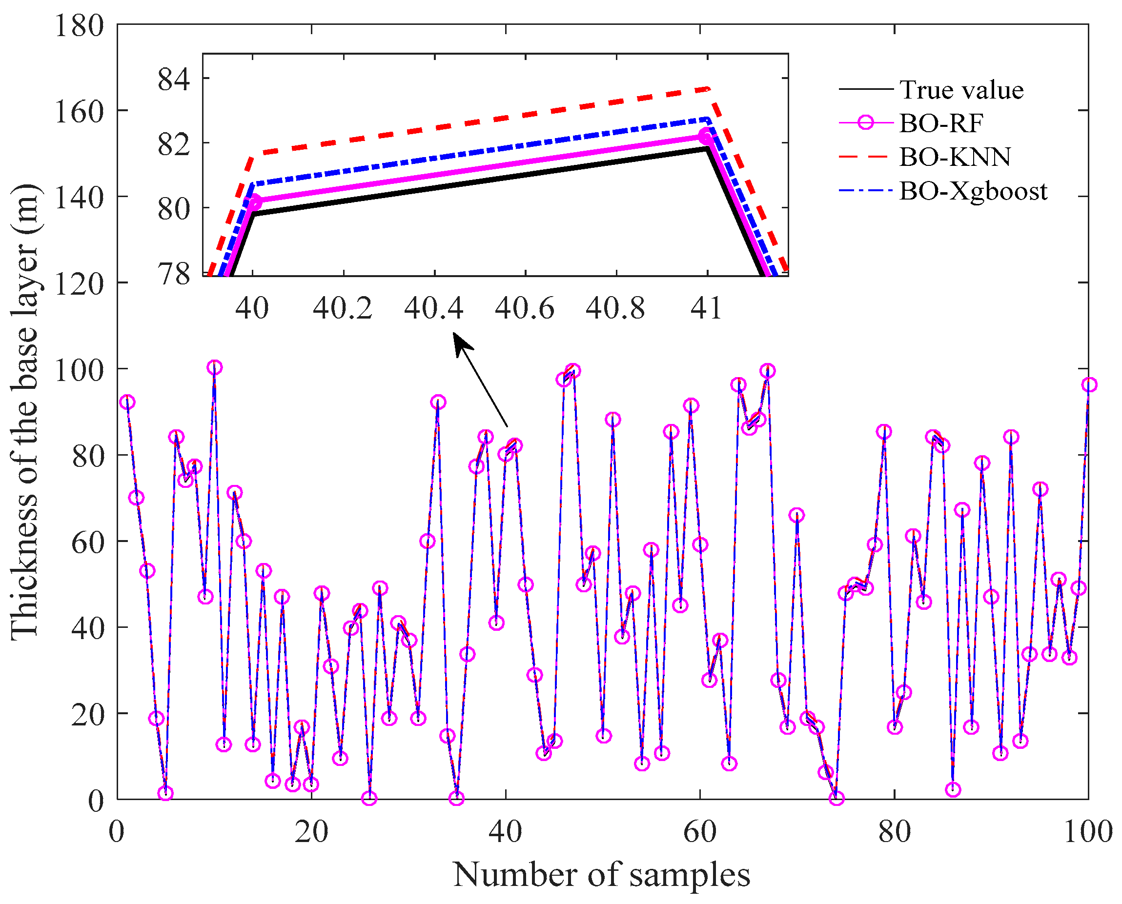
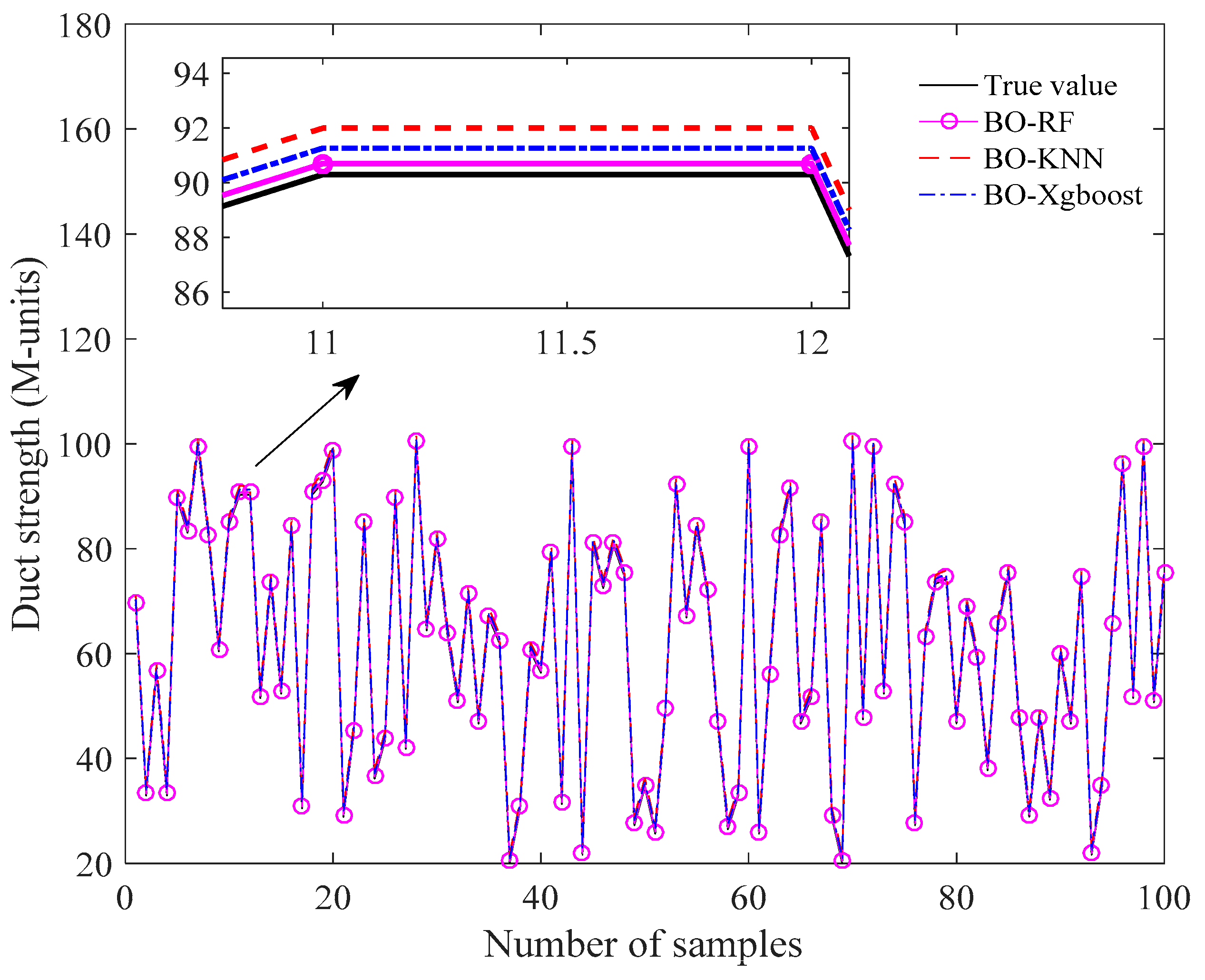
Furthermore, we randomly select 100 sets of predicted vectors of the refractivity parameter with 5% Gaussian noise from 2000 sets of predicted results to show the distributions of each parameter in SBD. From Figure 7, Figure 8 and Figure 9, it can be roughly observed that the predicted parameters, such as the thickness of the base layer, the thickness of the trapping layer, and the duct strength obtained with BO-RF, BO-KNN, and BO-XGBoost, are in good agreement with the true values. In order to carefully examine the performance of the three methods, the partial enlarged drawing in each figure is also provided. It is clearly shown that the BO-RF obtains the best performance compared with BO-KNN and BO-XGBoost.
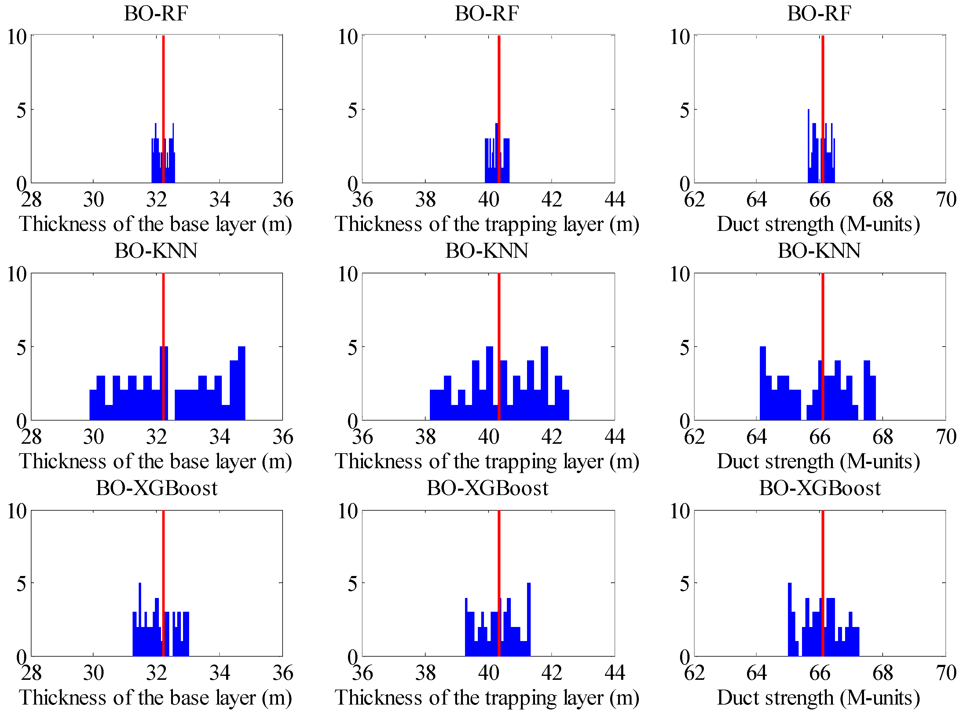
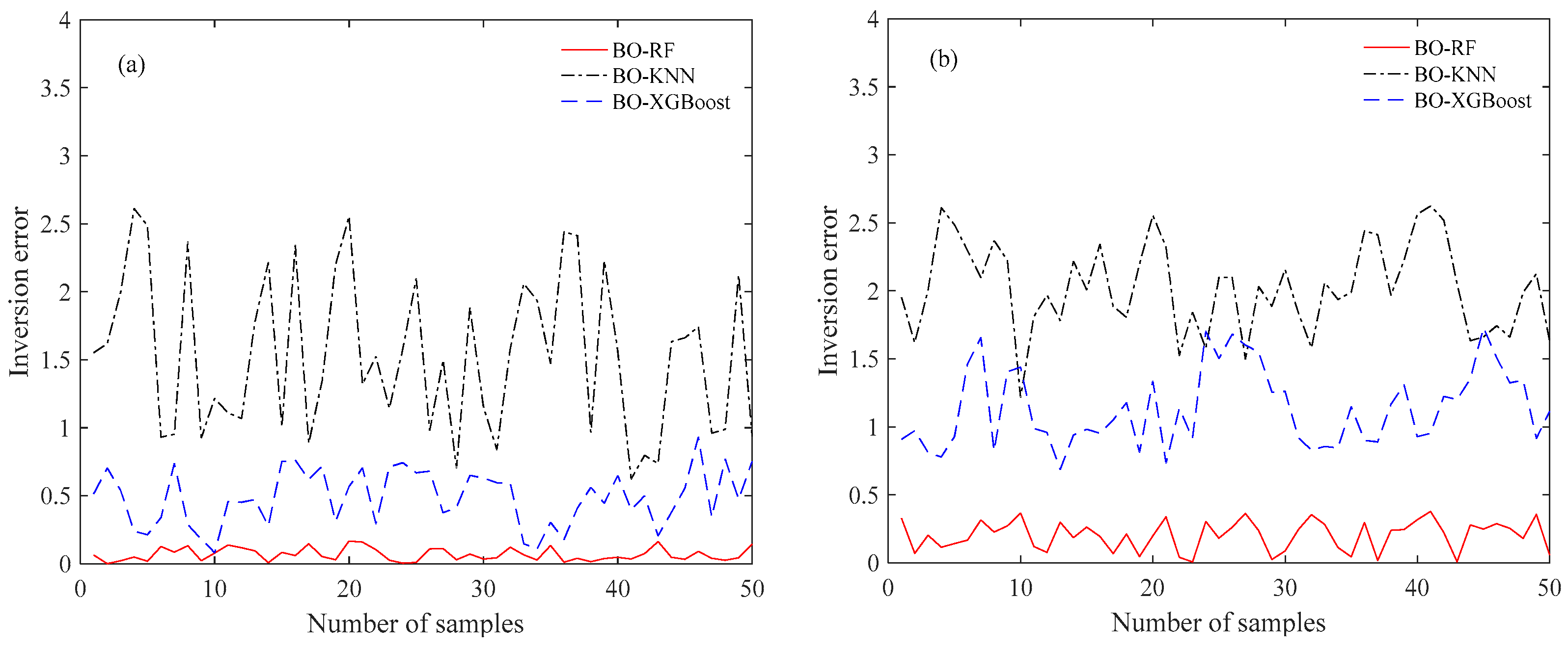
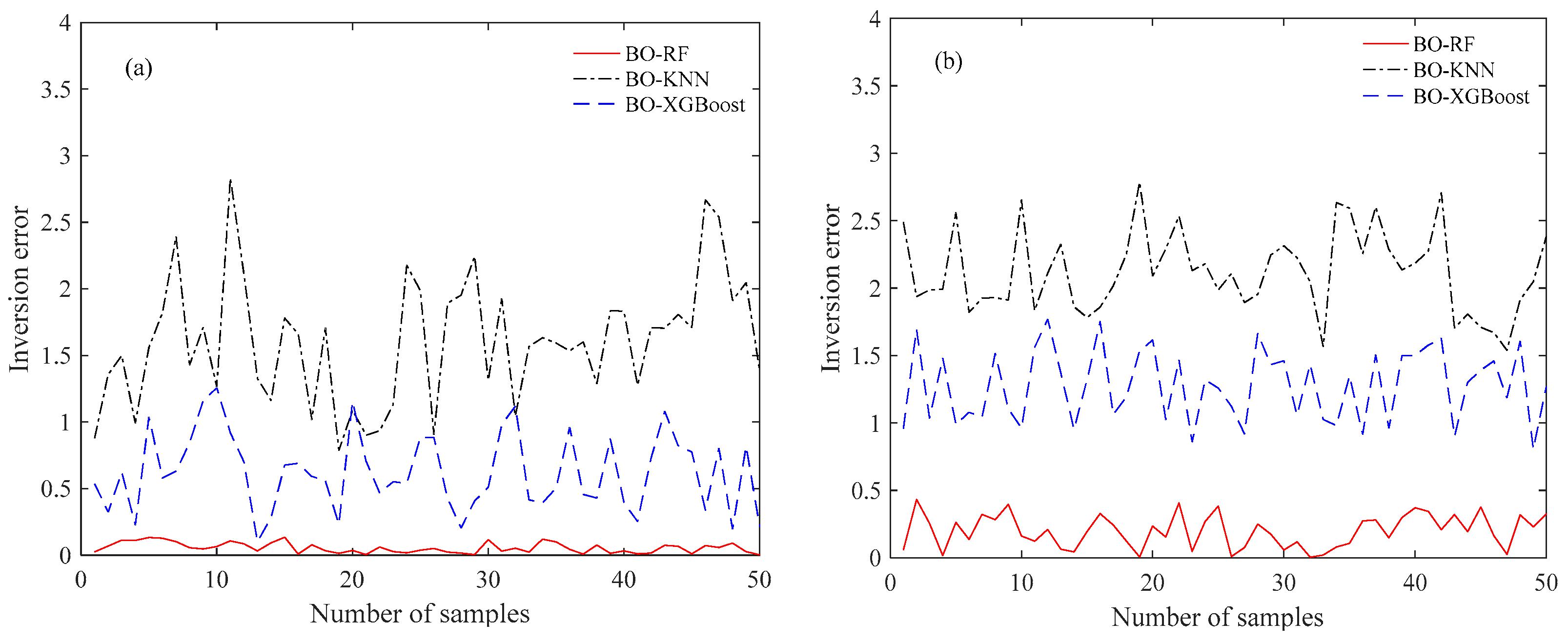
Another analysis focused on the accuracy and stability based on 50 independent runs for the inversion of SBD with/without 5% Gaussian noise is provided. Figure 10 and Figure 11 demonstrate the comparison of the histograms of the estimation results achieved by BO-RF, BO-KNN, and BO-XGBoost. It should be pointed out that the red lines denote the position of the true parameter in SBD. It can be seen that the estimation parameters of BO-RF distribute closely to the true parameter compared with the other two models; these mean that the performance of BO-RF performs better than those of BO-KNN and BO-XGBoost in the case of with/without noise. Additionally, the difference between the true and predicted parameters, named inversion error, for the thickness of the base layer, the thickness of the trapping layer, and the duct strength based on the above 50 independent runs is given in Figure 12, Figure 13 and Figure 14. It is clearly shown that the inversion error of BO-RF is also much lower than those of the two models; these also suggest that the accuracy of BO-RF is superior to those of BO-KNN and BO-XGBoost.
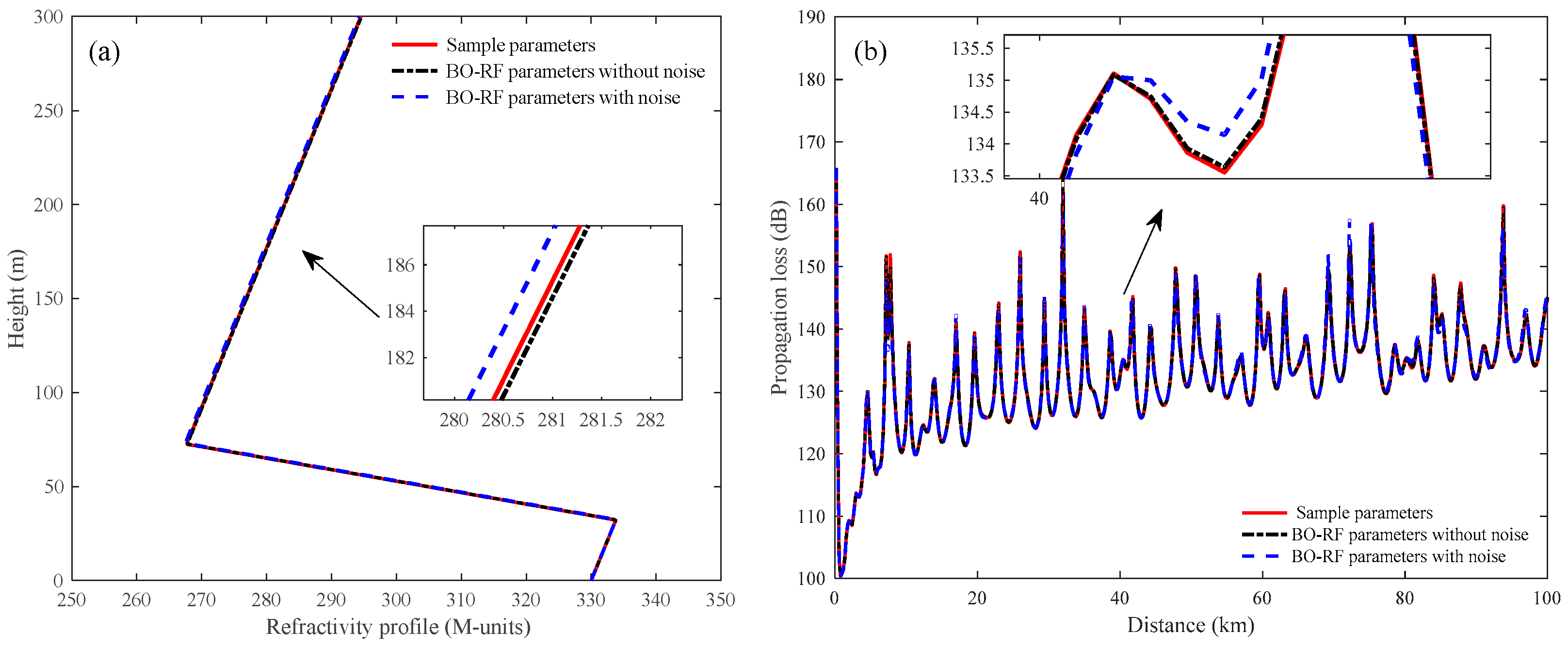
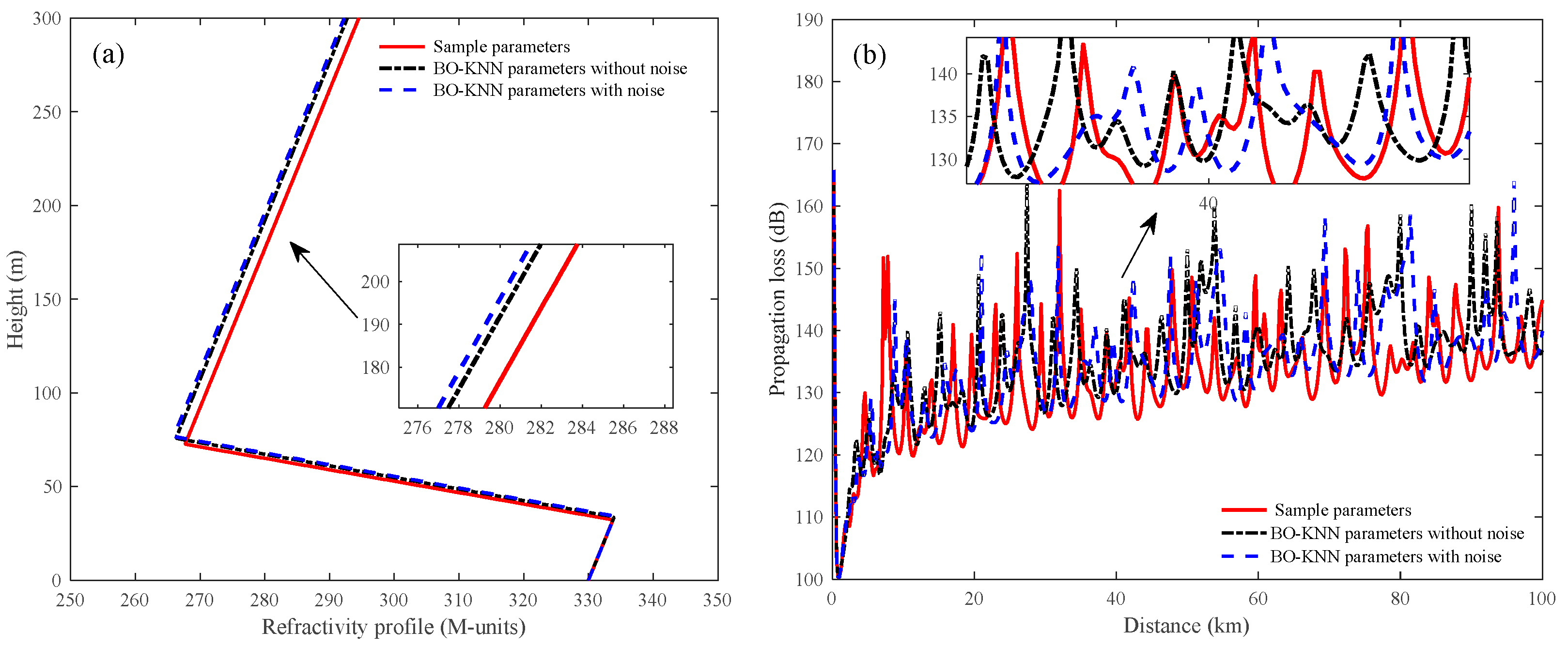
In addition, a comparative study focused on the refractivity profile and propagation loss between the true and predicted parameters in SBD is given in the subsequent section. The average inversion parameters of SBD with BO-RF, BO-KNN, and BO-XGBoost are given in Table 6.
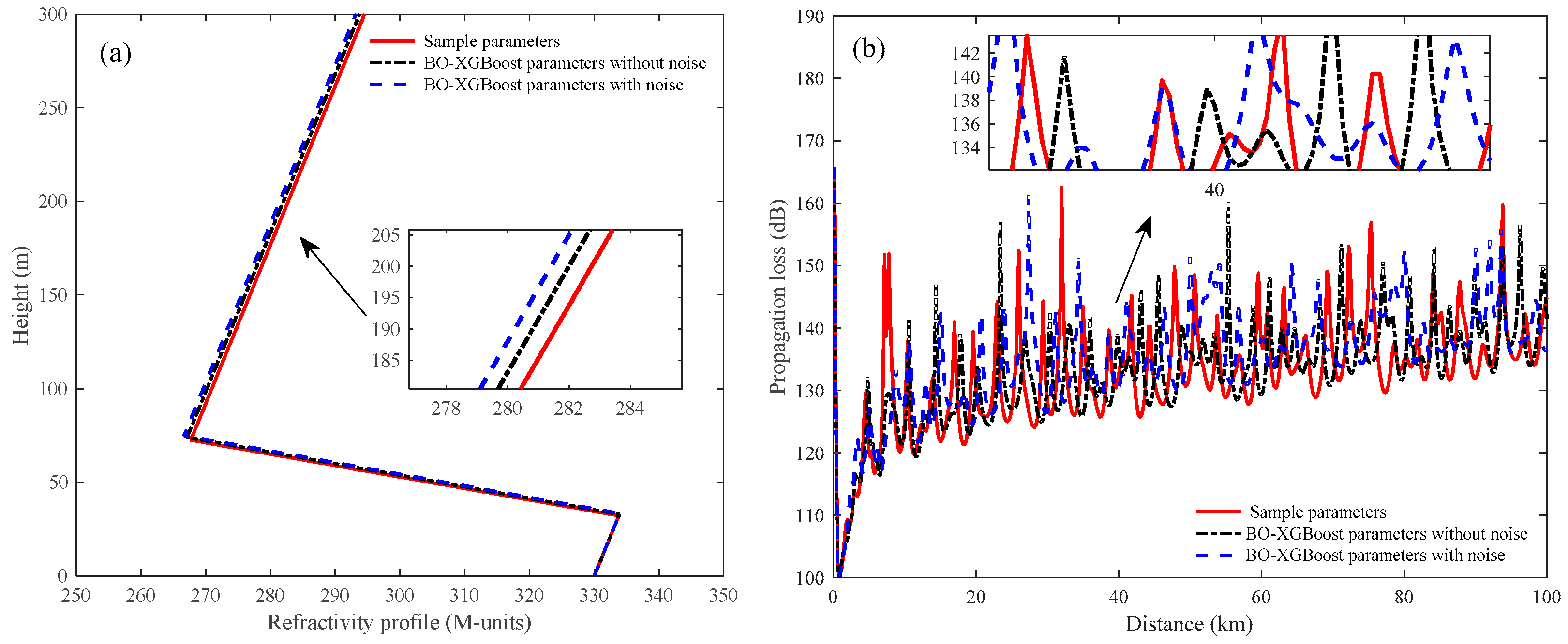
z b z t h i c k M d Figure 15, Figure 16 and Figure 17 give comparisons of the refractivity profile and propagation loss between the true and predicted parameters. Furthermore, a partial enlarged drawing of each figure is presented to exhibit the details. Compared with BO-KNN and BO-XGBoost, we can conclude that the predicted refractivity profiles and their propagation loss obtained with BO-RF exhibit good agreement with the results simulated with true parameters with/without noise. In addition, we can see from Figure 16 and Figure 17 that there are somewhat large deviations between the propagation loss simulated by the true and predicted parameters. This is due to the fact that a small variation in the index of refraction can cause a relatively large change in propagation loss.

6. Conclusions

The accurate inversion of atmospheric ducts is of great significance to the performance evaluation and design of radar and communication systems. In this paper, a BO-RF model is presented to predict the atmospheric duct parameters. Since the hyper-parameter plays a crucial role in the prediction performance of machine learning, BO is adopted to find the appropriate hyper-parameter in RF, and the results suggest that BO is an effective way to find the best hyper-parameter in RF. In addition, OED is used to sample the combinations of refractivity parameters from a range of hyper-parameter since it is a robust way to effectively handle multi-dimension sampling problems. To test the performance of the proposed BO-RF model, the results obtained by the BO-RF are compared with the results obtained by commonly used methods, such as classical RF, XGBoost with/without BO, and KNN with/without BO, with respect to the coefficient of determination R2, MAE, and MSE, as well as inversion error. The statistical and comparative analysis indicates that the BO-RF obtains the best results in the case with/without noise and outperforms the other algorithms adopted in this paper for the estimation of atmospheric duct parameters. Future work will mainly focus on the estimation study based on real data with machine learning and the improvement of the existing refractivity model.

Author Contributions

Conceptualization, C.Y.; methodology, A.Z.; software, A.Z. and Y.W.; validation, C.Y., Y.W. and A.Z.; formal analysis, Y.W.; investigation, Y.W.; resources, C.Y. and L.G.; data curation, Y.W. and A.Z.; writing—original draft preparation, A.Z.; writing—review and editing, C.Y. and Y.W.; visualization, Y.W., A.Z. and H.F.; supervision, C.Y.; project administration, C.Y. and L.G.; funding acquisition, C.Y. and L.G. All authors have read and agreed to the published version of the manuscript.

Funding

This research was funded by the National Natural Science Foundation of China (Grant Nos. 61871457, 61302050) and the Natural Science Foundation of Shaanxi Province (Grant No. 2019JQ-200).

Data Availability Statement

Not applicable.

Conflicts of Interest

The authors declare no conflict of interest.

References

  1. Yardim, C.; Gerstoft, P.; Hodgkiss, W.S. Estimation of radio refractivity from radar clutter using Bayesian Monte Carlo analysis. IEEE Trans. Antennas Propag. 2006, 54, 1318–1327. [Google Scholar] [CrossRef]
  2. Gerstoft, P.; Rogers, L.T.; Krolik, J.L.; Hodgkiss, W.S. Inversion for refractivity parameters from radar sea clutter. Radio Sci. 2003, 38, 1801–1822. [Google Scholar] [CrossRef]
  3. Karimian, A.; Yardim, C.; Gerstoft, P.; Hodgkiss, W.S.; Barrios, A.E. Refractivity estimation from sea clutter: An invited review. Radio Sci. 2011, 46, RS6013. [Google Scholar]
  4. Douvenot, R.; Fabbro, V.; Gerstoft, P.; Bourlier, C.; Saillard, J. A duct mapping method using least squares support vector machines. Radio Sci. 2008, 43, RS6005. [Google Scholar] [CrossRef]
  5. Wang, B.; Wu, Z.S.; Zhao, Z.; Wang, H.G. Retrieving evaporation duct heights from radar sea clutter using particle swarm optimization (PSO) algorithm. Prog. Electromagn. Res. M 2009, 9, 79–91. [Google Scholar] [CrossRef]
  6. Zhang, J.P.; Wu, Z.S.; Zhu, Q.L.; Wang, B. A four-parameter M-profile model for the evaporation duct estimation from radar clutter. Prog. Electromagn. Res. 2011, 114, 353–368. [Google Scholar] [CrossRef]
  7. Zhao, X. Evaporation duct height estimation and source localization from field measurements at an array of radio receivers. IEEE Trans. Antennas Propag. 2011, 60, 1020–1025. [Google Scholar] [CrossRef]
  8. Yang, C. Estimation of the atmospheric duct from radar sea clutter using artificial bee colony optimization algorithm. Prog. Electromagn. Res. 2013, 135, 183–199. [Google Scholar] [CrossRef]
  9. Yang, C.; Guo, L. Inferring the atmospheric duct from radar sea clutter using the improved artificial bee colony algorithm. Int. J. Microw. Wireless Technol. 2018, 10, 437–445. [Google Scholar]
  10. Yang, C.; Wang, Y. Inversion of the surface duct from radar sea clutter using the improved whale optimization algorithm. Electromagnetics 2019, 39, 611–627. [Google Scholar] [CrossRef]
  11. Yang, C. A comparison of the machine learning algorithm for evaporation duct estimation. Radioengineering 2013, 22, 657–661. [Google Scholar]
  12. Tepecik, C.; Navruz, I. A novel hybrid model for inversion problem of atmospheric refractivity estimation. Int. J. Electron. Commun. 2018, 84, 258–264. [Google Scholar] [CrossRef]
  13. Lentini, N.E.; Hackett, E.E. Global sensitivity of parabolic equation radar wave propagation simulation to sea state and atmospheric refractivity structure. Radio Sci. 2015, 50, 1027–1049. [Google Scholar] [CrossRef]
  14. Penton, S.E.; Hackett, E.E. Rough ocean surface effects on evaporative duct atmospheric refractivity inversions using genetic algorithms. Radio Sci. 2018, 53, 804–819. [Google Scholar] [CrossRef]
  15. Pozderac, J.; Johnson, J.; Yardim, C.; Merrill, C.; Paolo, T.; Terrill, E.; Ryan, F.; Frederickson, P. X-band Beacon-receiver array evaporation duct height estimation. IEEE Trans. Antennas Propag. 2018, 66, 2545–2556. [Google Scholar] [CrossRef]
  16. Yan, X.; Yang, K.; Ma, Y. Calculation method for evaporation duct profiles based on artificial neural network. IEEE Antennas Wireless Propag. Lett. 2018, 17, 2274–2278. [Google Scholar] [CrossRef]
  17. Zhu, X.; Li, J.; Zhu, M.; Jiang, Z.; Li, Y. An evaporation duct height prediction method based on deep learning. IEEE Trans. Geosci. Remote Sens. 2018, 15, 1307–1311. [Google Scholar] [CrossRef]
  18. Sit, H.; Earls, C.J. Characterizing evaporation ducts within the marine atmospheric boundary layer using artificial neural networks. Radio Sci. 2019, 54, 1181–1191. [Google Scholar] [CrossRef]
  19. Sit, H.; Earls, C.J. Deep Learning for Classifying and Characterizing Atmospheric Ducting within the Maritime Setting. Comput. Geosci. 2021, 157, 104919. [Google Scholar] [CrossRef]
  20. Belgiu, M.; Drăguţ, L. Random forest in remote sensing: A review of applications and future directions. ISPRS J. Photogramm. Remote Sens. 2016, 114, 24–31. [Google Scholar] [CrossRef]
  21. Onan, A.; Korukoğlu, S.; Bulut, H. Ensemble of keyword extraction methods and classifiers in text classification. Expert Syst. Appl. 2016, 57, 232–247. [Google Scholar] [CrossRef]
  22. Kumari, P.; Toshniwal, D. Extreme gradient boosting and deep neural network based ensemble learning approach to forecast hourly solar irradiance. J. Clean. Prod. 2021, 279, 123285. [Google Scholar] [CrossRef]
  23. Song, Y.; Liang, J.; Lu, J.; Zhao, X. An efficient instance selection algorithm for k nearest neighbor regression. Neurocomputing 2017, 251, 26–34. [Google Scholar] [CrossRef]
  24. Alberoni, P.P.; Andersson, T.; Mezzasalma, P.; Michelson, D.B.; Nanni, S. Use of the vertical reflectivity profile for identification of anomalous propagation. Meteorol. Appl. 2001, 8, 257–266. [Google Scholar] [CrossRef]
  25. Bech, J.; Sairouni, A.; Codina, B.; Lorente, J.; Bebbington, D. Weather radar anaprop conditions at a Mediterranean coastal site. Phys. Chem. Earth B 2000, 25, 829–832. [Google Scholar] [CrossRef]
  26. Karimian, A.; Yardim, C.; Hodgkiss, W.S.; Gerstoft, P.; Barrios, A.E. Estimation of radio refractivity using a multiple angle clutter model. Radio Sci. 2012, 47, 1–9. [Google Scholar] [CrossRef]
  27. Sirkova, I. Brief review on PE method application to propagation channel modeling in sea environment. Open Eng. 2012, 2, 19–38. [Google Scholar] [CrossRef]
  28. Levy, M.F. Parabolic Equation Methods for Electromagnetic Wave Propagation; Institution of Engineering and Technology: London, UK, 2000. [Google Scholar]
  29. Dockery, G.D. Modeling electromagnetic wave propagation in the troposphere using the parabolic equation. IEEE Trans. Antennas Propag. 1988, 36, 1464–1470. [Google Scholar] [CrossRef]
  30. Adusumilli, S.; Bhatt, D.; Wang, H.; Bhattacharya, P.; Devabhaktuni, V. A low-cost INS/GPS integration methodology based on random forest regression. Expert Syst. Appl. 2013, 40, 4653–4659. [Google Scholar] [CrossRef]
  31. Rafe, V.; Mohammady, S.; Cuevas, E. Using Bayesian optimization algorithm for model-based integration testing. Soft Comput. 2021, 26, 3503–3525. [Google Scholar] [CrossRef]
  32. Ziatdinov, M.A.; Ghosh, A.; Kalinin, S.V. Physics makes the difference: Bayesian optimization and active learning via augmented Gaussian process. Mach. Learn. Sci. Technol. 2022, 3, 015022. [Google Scholar] [CrossRef]
  33. Gao, W.; Liu, S.; Huang, L. A novel artificial bee colony algorithm based on modified search equation and orthogonal learning. IEEE Trans. Cybern. 2013, 43, 1011–1024. [Google Scholar]
  34. Wang, Y.; Cai, Z.X.; Zhang, Q.F. Enhancing the search ability of differential evolution through orthogonal crossover. Inf. Sci. 2012, 185, 153–177. [Google Scholar] [CrossRef]
  35. Zhan, Z.H.; Zhang, J.; Li, Y.; Shi, Y.H. Orthogonal learning particle swarm optimization. IEEE Trans. Evol. Comput. 2011, 15, 832–847. [Google Scholar] [CrossRef]
  36. Moreta, C.E.G.; Acosta, M.R.C.; Koo, I. Prediction of digital terrestrial television coverage using machine learning regression. IEEE Trans. Broadcast. 2019, 65, 702–712. [Google Scholar] [CrossRef]
  37. Chicco, D.; Warrens, M.J.; Jurman, G. The coefficient of determination R-squared is more informative than SMAPE, MAE, MAPE, MSE and RMSE in regression analysis evaluation. PeerJ Comput. Sci. 2021, 7, e623. [Google Scholar] [CrossRef]
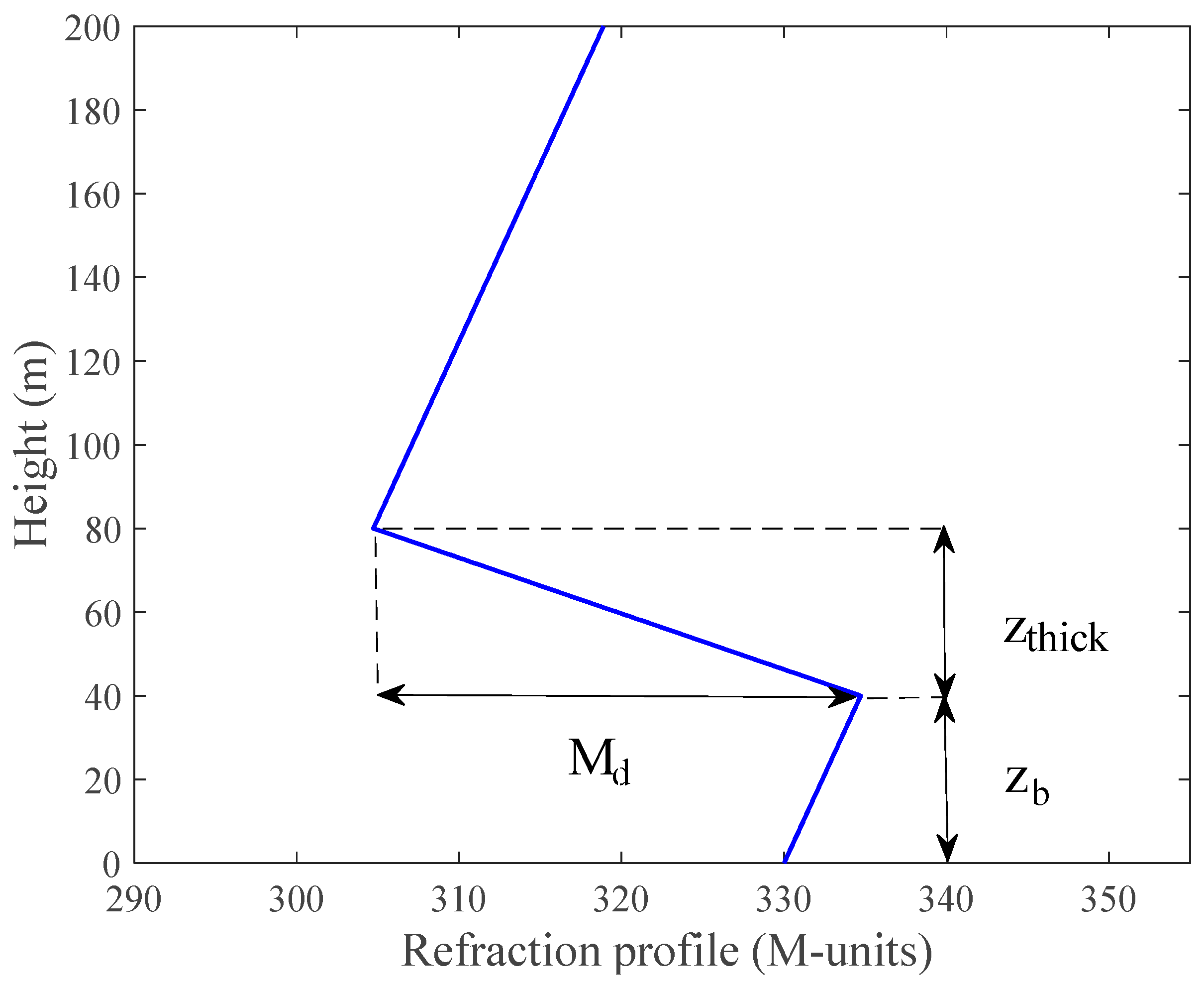
Figure 1. Tri-linear refractivity profile for SBD.
Remotesensing 15 04296 g001
Figure 2. Flowchart of the BO-RF for atmospheric duct estimation.
Remotesensing 15 04296 g002
Figure 3. Curve of the RSCP versus the propagation distance at different receiving heights.
Remotesensing 15 04296 g003
Figure 4. Comparison of the coverage diagrams for different thicknesses of the base layer.
Remotesensing 15 04296 g004
Figure 5. Comparison of the coverage diagrams for different thicknesses of the trapping layer.
Remotesensing 15 04296 g005
Figure 6. Comparison of the coverage diagrams for different duct strength.
Remotesensing 15 04296 g006
Figure 7. Comparison of the predicted thicknesses of the base layer for the BO-optimized models.
Remotesensing 15 04296 g007
Figure 8. Comparison of the predicted thicknesses of the trapping layer for the BO-optimized models.
Remotesensing 15 04296 g008
Figure 9. Comparison of the predicted duct strength for the BO-optimized models.
Remotesensing 15 04296 g009
Figure 10. Comparison of the histograms of BO-RF, BO-KNN, and BO-XGBoost without noise.
Remotesensing 15 04296 g010
Figure 11. Ccomparison of the histograms of BO-RF, BO-KNN, and BO-XGBoost with 5% Gaussian noise.
Remotesensing 15 04296 g011
Figure 12. Comparison of the inversion error with the thickness of the base layer: (a) without noise and (b) with 5% Gaussian noise.
Remotesensing 15 04296 g012
Figure 13. Comparison of the inversion error with the thickness of the trapping layer: (a) without noise and (b) with 5% Gaussian noise.
Remotesensing 15 04296 g013
Figure 14. Comparison of the inversion error with the duct strength: (a) without noise and (b) with 5% Gaussian noise.
Remotesensing 15 04296 g014
Figure 15. Comparison of the (a) refractivity profile and (b) propagation loss between the true and predicted parameters obtained by BO-RF.
Remotesensing 15 04296 g015
Figure 16. Comparison of the (a) refractivity profile and (b) propagation loss between the true and predicted parameters obtained by BO-KNN.
Remotesensing 15 04296 g016
Figure 17. Comparison of the (a) refractivity profile and (b) propagation loss between the true and predicted parameters obtained by BO-XGBoost.
Remotesensing 15 04296 g017
Table 1. Range of hyper-parameter in RF.
DescriptionHyper-ParameterSearch Range
number of decision treesn_estimator(10, 500)
maximum depth of treesmax_depth(5, 50)
minimum samples of splitmin_sample_split(1, 50)
minimum samples of leafmin_sample_leaf(1, 50)
maximum number of featuresmax_features(4, 100)
Table 2. Radar system parameters.
ParametersValue
Frequency2.84 GHz
Transmitting power91.4 dBm
Beamwidth0.4°
Antenna height30.78 m
Transmitting antenna gain52.8 dB
PolarizationVV
Table 3. Default and BO-optimized hyper-parameter.
Hyper-ParameterDefault ValueOptimized Value
n_estimator30382
max_depth642
min_sample_split42
min_sample_leaf41
max_featuresauto50
Table 4. Coefficient of determination R2 for the regression model.
AlgorithmsR2 without NoiseR2 with Noise
RF98.92%98.46%
BO-RF99.93%99.82%
KNN90.67%87.51%
BO-KNN91.76%88.72%
XGBoost94.68%93.73%
BO-XGBoost95.96%94.83%
Table 5. Comparison of the MAE and MSE for the test results without noise and with 5% Gaussian noise.
AlgorithmsParametersMAEMSE
Without NoiseWith 5% Gaussian NoiseWithout NoiseWith 5% Gaussian Noise
RF z b /m0.480.490.440.82
z t h i c k /m0.350.670.711.18
M d /M-units0.480.500.400.95
BO-RF z b /m0.140.390.050.62
z t h i c k /m0.090.360.060.51
M d /M-units0.160.400.090.84
KNN z b /m1.571.913.637.24
z t h i c k /m1.962.098.448.37
M d /M-units2.612.859.579.91
BO-KNN z b /m1.471.853.455.30
z t h i c k /m1.761.845.646.03
M d /M-units2.462.706.308.80
XGBoost z b /m0.931.062.784.00
z t h i c k /m1.421.694.074.15
M d /M-units1.121.673.555.06
BO-XGBoost z b /m0.640.911.163.14
z t h i c k /m0.750.902.112.79
M d /M-units0.980.972.082.97
Table 6. Average inversion results of SBD.
ParametersBO-RFBO-KNNBO-XGBoost
Without NoiseNoiseWithout NoiseNoiseWithout NoiseNoise
z b /m32.2832.4333.7734.2632.9233.37
z t h i c k /m40.3040.5441.9542.4441.1041.62
M d /M-units66.0366.3367.6968.1166.7667.28
Disclaimer/Publisher’s Note: The statements, opinions and data contained in all publications are solely those of the individual author(s) and contributor(s) and not of MDPI and/or the editor(s). MDPI and/or the editor(s) disclaim responsibility for any injury to people or property resulting from any ideas, methods, instructions or products referred to in the content.