Three-Dimensional Reconstruction and Geometric Morphology Analysis of Lunar Small Craters within the Patrol Range of the Yutu-2 Rover

Abstract

Craters on the lunar surface are the most direct method for the study of geological processes and are of great significance to the study of lunar evolution. In order to fill the research gap on small craters (diameter less than 3 m), we focus on the small craters around the moving path of the Yutu-2 lunar rover and carry out a 3D reconstruction and geometrical morphology analysis on them. First, a self-calibration model with multiple feature constraints is used to calibrate the navigation camera and obtain the internal and external parameters. Then, the sequence images with overlapping regions from neighboring stations are used to obtain the precise position of the rover through the bundle adjustment (BA) method. After that, a cross-scale cost aggregation for a stereo matching network is proposed to obtain a parallax map, which can further obtain 3D point clouds of the lunar surface. Finally, the indexes of the craters are extracted (diameter D, depth d, and depth–diameter ratio d_r), and the different indicators are fitted and analyzed. The results suggest that CscaNet has an anomaly percentage value of 1.73% in the KITTI2015 dataset, and an EPE of 0.74 px in the SceneFlow dataset, both of which are superior to GC-Net, DispNet, and PSMnet, and have higher reconstruction accuracy. The correlation between D and d is high and exhibits a positive correlation, while the correlation between D and d_r is low. The geometric morphology expressions of small craters fitted by using D and d are significantly different from the expressions proposed by other scholars for large craters. This study provides a priori knowledge for the subsequent Von Karmen crater survey mission in the SPA Basin.

1. Introduction

The lunar surface is widely littered with craters of all sizes and shapes. Each crater is composed of six main parts: a bottom, a wall, an uplift edge, a central uplift, radiation stripes, and sputters [1]. An in-depth study of crater morphology, including the shape, size, and distribution of craters, can provide important information about the internal structure, rock composition, and geological processes of the Moon, and can also be analyzed to learn about impact events of different sizes and frequencies on the Moon to help us understand the early formation and evolution of the solar system [2]. Due to special environmental factors such as the Moon having no water, wind, or atmosphere, crater information has been preserved. During the Chang’e-1 mission from China, based on the gravity field anomaly model, it was inferred that there was a mascon directly below the Von Karman Crater at the south pole of the Moon and that the geological composition of the mascon was relatively complicated. The discovery of such hidden lunar mascons provides extremely important basic data for human research on the formation and geology of the Moon [2]. Therefore, analyzing the geometry of craters has become a direct entry point for studying the evolution and development of lunar morphological features.

Due to limited data sources, current studies focus on medium- and large-sized craters with a diameter greater than 0.1 km. Head [3,4] and Kadish et al. [5] created a list of 5185 craters with diameters of more than 20 km in diameter on the lunar surface based on the data from the lunar orbiter laser altimeter (LOLA) system. McDowell et al. [6] identified 8639 craters on the Moon. Salamuniccar et al. [7] established the LU60645GT list of 60,645 craters. Robbins et al. [8] established a lunar crater database containing 2,033,574 craters. In subsequent studies, Robbins et al. [9] measured small craters (ranging from 10 m to 500 m in diameter) in the lunar mare region and larger craters (ranging from 100 m to 1 km in diameter) in the lunar highland and lunar mare regions. Wang et al. [10] identified 106,016 lunar craters with diameters greater than 500 m based on public data from the Chang’e lunar exploration project and analyzed the differences and distribution rules of lunar craters in different spatial scales. Hou et al. [11] used the Chang’e-1 digital elevation model (DEM) data to analyze the spatial distribution of craters over the entire surface of the Moon by examining the numbers of craters in different diameter intervals and demonstrated that there were enormous numbers of medium-sized and small craters. Li et al. [12] summarized and analyzed the structural characteristics of craters, the concept and behavioral characteristics of crater families, and the relationship between craters and stratigraphic age based on the morphological and evolutionary characteristics of 100-meter-level craters.

In addition, scholars have carried out research on crater recognition. Zhao [13] proposed an intelligent recognition method based on region-based fully convolutional networks (R-FCNs) for identifying craters with diameters of less than 1 km. Zuo et al. [14] used the contrast, highlight, and shadow features of craters in the sunlight to automatically identify small lunar craters. Hu [15] proposed the semantic segmentation of the digital elevation model to detect small craters. Kang [16] proposed a coarse-to-fine resolution recognition method. In this method, first, the histogram of oriented gradient (HOG) features and a support vector machine (SVM) classifier are used to conduct preliminary classification; then, small craters are automatically identified from charge-coupled device (CCD) images. Yang recognized 20,000 small craters through deep learning [17].

For the geometric modeling of craters, previous studies have demonstrated that morphological parameters such as the depth, edge height, and central peak height of complex craters change exponentially with diameter [18]; the basic expression is $y=a{D}^b$, where $y$ represents a morphological characteristic value of a given crater, such as its depth, edge height, edge width, central peak height, crater volume, or bottom area; $D$ denotes the diameter of the crater; and $a$ and $b$ are constants. In view of the morphological characteristics of newly formed craters with high correlations, Bouska, Head, Pike, and Hu et al. [19,20,21,22,23,24,25] used data obtained by different detectors to intensively study the newly formed original craters or secondary craters in different regions and presented the correlation equations of the shape parameters of various craters. Baldwin et al. studied the morphological relationship of craters in the early stage and obtained the expression D = 0.256d² + d + 0.6300. Bouska et al. identified the morphological relationship expression of craters as logD = Alogd + B (where A and B are coefficients to be determined). Pike et al. obtained an expression for the morphological relationship of craters with diameters of less than 15 km, namely, d = 0.196d^1.010. Hu et al. obtained morphological relationship expressions for simple craters, namely, d = 0.126D + 0.4902, and for complex craters, d = 0.3273D^0.6252. Early crater depth data were obtained mainly by shadow length measurement. With the development of science and technology, depth data have become acquired through LOLA, which has improved the resolution and accuracy, and the identification rate and number of identified craters have increased greatly. Based on new data sources, more in-depth studies have been carried out on the geometry of craters. Hu et al. began to analyze the morphological characteristics of craters in different regions based on the differences in the morphological characteristics of different types of craters.

However, in the geometric analysis of craters, the following problems are still encountered: (1) Available lunar remote sensing images cannot be used to accurately identify the geometries of small craters (less than 3 m in diameter) and no solution to this problem has been found in related research. (2) It remains to be quantitatively studied whether the geometric modeling and metric data for small craters on the far side of the Moon are consistent with those of traditional large craters (less than 10 km in diameter). (3) Limited by the available data sources, the geometric modeling accuracy for the small craters on the far side of the Moon is low, and performing high-precision geometric morphological modeling is of necessity.

During the Chang’e-4 mission, the Yutu-2 lunar rover collected detailed images of the far side of the Moon in the Von Karman Crater region in the SPA Basin, which provided basic data for studying the geometric modeling of small craters on the far side of the Moon. This is the core step of the geometric modeling process for building a fine three-dimensional model of small craters. The process generally includes camera calibration, visual positioning of the lunar rover, stereo matching, and 3D modeling. In the field of camera calibration, Zhang et al. [26] proposed a method based on three-dimensional direct linear transformation (DLT) and multi-image rear intersection iterative computation for accurate lunar rover calibration. Xu et al. [27] built a combined adjustment model for the self-calibrated beam method which includes distance constraints, collinearity and coplanarity conditions, and relative pose constraints of the stereo camera. With solar panels as calibration targets, after the rover landing, Yan et al. [28] proposed using grid lines as a calibration method for linear parameters by applying the Hough transform, a clustering strategy, and least squares linear fitting. In the field of visual positioning, Wang et al. [29] proposed using scale-invariant feature transform (SIFT) matching for interstation image matching, combining the correlation coefficient and least squares matching to achieve feature matching of the same interstation image, and finally using the beam adjustment method to realize relative positioning between two stations. Liu et al. [30] used affine scale-invariant feature transform (Affine-SIFT) matching with the beam adjustment model to realize relative positioning between two stations. Ma et al. [31] used the unit quaternion beam adjustment model and virtual observation to obtain an accurate calculation adjustment model of the Mars rover and to achieve continuous relative positioning of the rover. In the field of stereo matching, Li et al. [32] et al. proposed the three-dimensional reconstruction of the lunar surface terrain using an improved dynamic programming method for stereo matching in view of the unique imaging environment of the lunar surface, which has characteristics such as sparse texture, low illumination, and occlusion, and demonstrated that the image matching algorithm directly affects the accuracy and reliability of terrain restoration. Cao et al. [33], aiming at satisfying the real-time performance and reliability requirements of the lunar rover vision system, proposed using Gaussian filtering and the contrast-limited adaptive histogram equalization (CLAHE) method to preprocess stereoscopic images, using the SIFT to extract the point and edge features, and calculating the three-dimensional information of the lunar environment by matching joint points with edge features. Hou et al. [34] proposed a feature-assisted region-matching algorithm, using the regional feature constraints of less-texture and no-texture regions through regional matching, combining the advantages of respective matching. Peng et al. proposed an adaptive Markov random field model to constrain the parallax range of texture-poor deep space detection images [35]; the adaptive method reduces the scope of the parallax search and preserves the parallax features in discontinuous regions. In recent years, scholars have proposed stereo-matching methods based on deep learning theory [36,37,38,39]. Zbontar et al. proposed the matching cost convolutional neural network (MC-CNN) algorithm [36] in which deep learning is introduced into stereo matching to design two network structures: MC-CNN-accurate architecture (MC-CNN-acrt) and MC-CNN-fast architecture (MC-CNN-fst). The algorithm uses a deep neural network to perform similarity metric learning on image features in image blocks and trains them in a supervised manner. Mayer et al. [37] proposed an end-to-end stereo matching algorithm, the disparity estimation network (DispNet) algorithm. The algorithm uses a codec-decoding structure with a cascading method for parallax regression, and a dataset, namely, Scene Flow, synthesized by stereo matching with a convolutional neural network used to pre-train the stereo-matching model of the convolutional neural network. Kendall et al. [38] proposed an algorithm based on cost volume aggregation, the geometry and context network (GC-Net). The cost volume is constructed by connecting the parallax of the feature dimensions, and a 3D convolutional neural network is used to regularize the constructed cost volume, while a codec structure is used to reduce false stereo matching. Chang et al. [39] proposed an algorithm based on pyramid stereo matching, namely, the pyramid stereo matching network (PSMNet) algorithm. This algorithm uses feature information aggregation at different scales and orientations to extract the global context information of images and employs a 3D hourglass structure to standardize the cost volume, thereby yielding a parallax map that is superior to that of GC-Net. These methods can solve the image matching problem but, due to the sparse and single lunar texture, the stereo matching accuracy is low; in particular, the lunar detail reconstruction performance is poor.

To realize the fine modeling of small craters on the far side of the Moon, a high-precision three-dimensional model of the small craters around the rover’s moving path is established by using stereo navigation camera images from the Yutu-2 lunar rover, and the geometric pattern of the small craters is studied [3,4,5,6,7,8,9,10,11,12]. The contributions of the proposed method comprise the following:

(1)

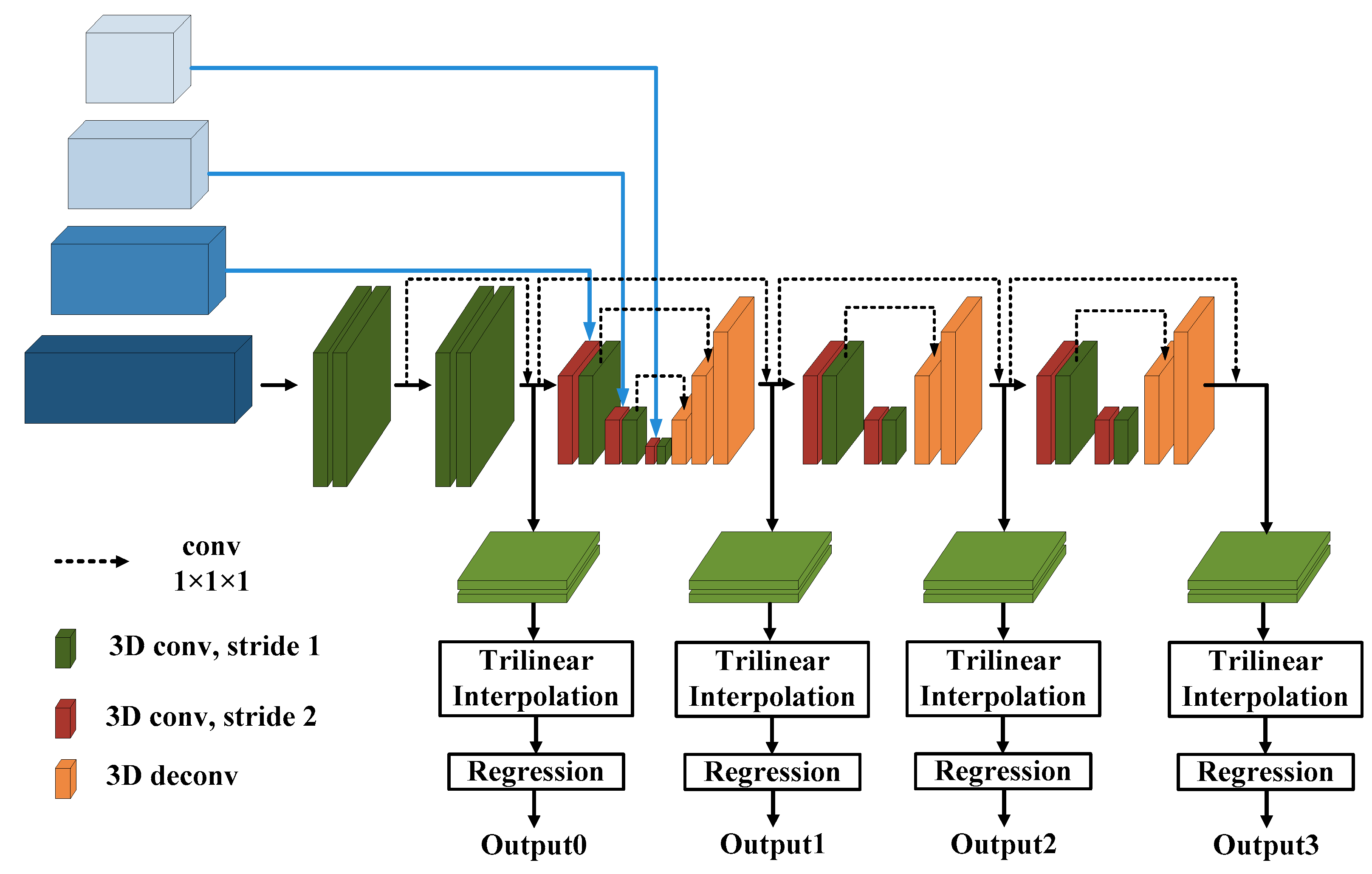
Considering the single sparse texture feature of the lunar surface, the cross-scale cost aggregation for a stereo matching network (CscaNet) is proposed.

(2)

For the first time, the proposed CscaNet and forward intersection [40] (triangulation) method is used to reconstruct the fine lunar terrain based on the image data obtained by the navigation camera. The small craters within the range are extracted, and a geometric morphological law analysis is carried out, which fills the gap in the morphological analysis of craters in the dorsal region of the Moon at the miniature scale.

(3)

For the first time, the geometric pattern of small craters is discovered, and the relationship between the depth and diameter of craters within the scope of the Yutu-2 patrol mission is analyzed.

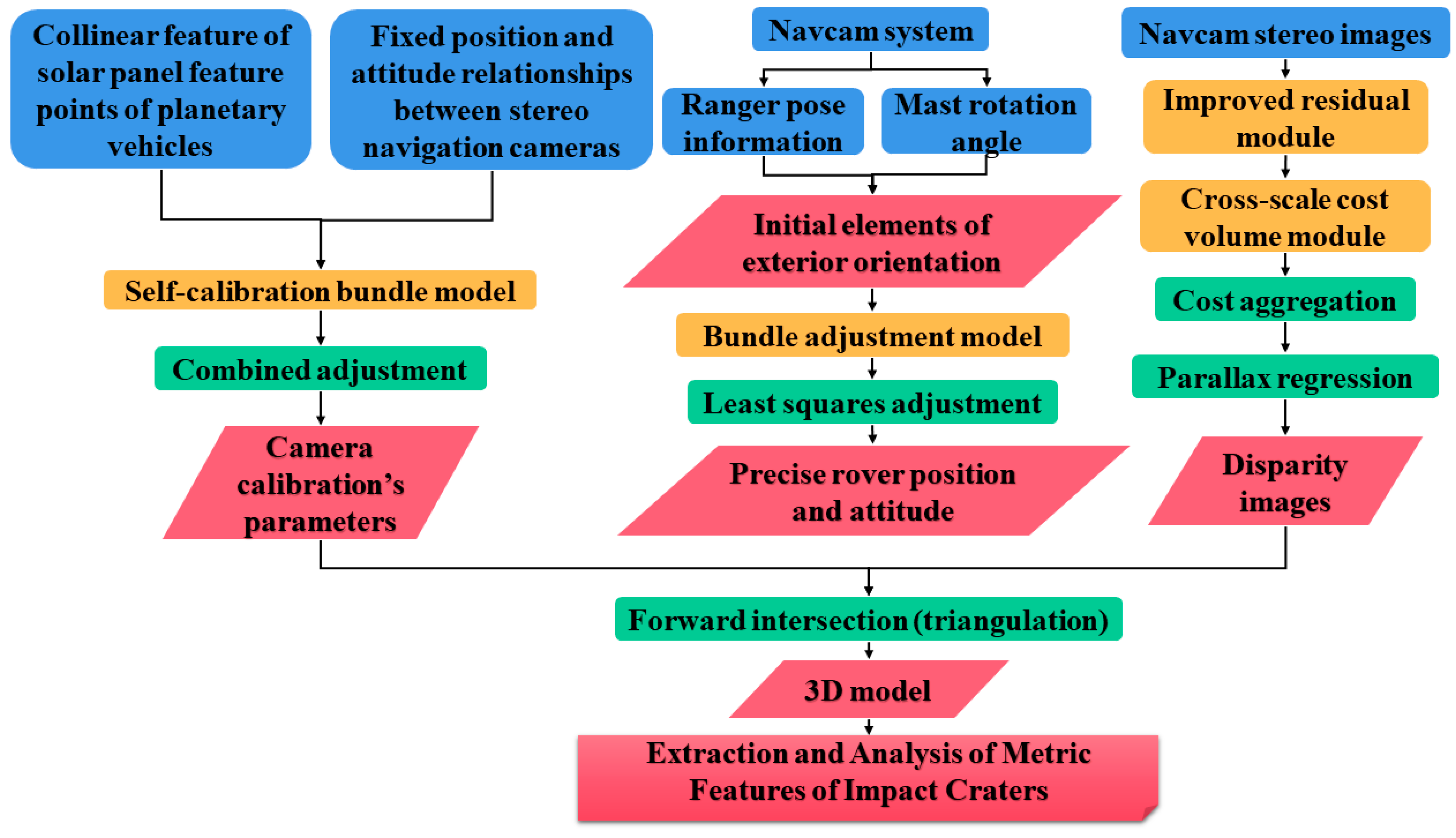
2. Methodology

The geometric modeling method for craters on the far side of the Moon proposed in this study first calibrates the lunar rover navigation camera based on the self-calibrated beam method combined with an adjustment model to obtain the internal and external parameters. Second, a visual positioning model of the lunar rover is built by using the sequence images with overlap regions of the adjacent exposure stations to accurately position the rover. Third, the CscaNet algorithm is used to obtain the image parallax map, which solves the problem of poor image matching caused by the simplex lunar image texture. On this basis, the parallax map is subjected to forward intersection to yield a 3D point cloud model of the lunar surface. Finally, the metric data (crater diameter, $D$; crater depth, d; and depth–diameter ratio, ${ d}_r=d/D$) of small craters are obtained based on the 3D point cloud of the lunar surface to analyze the small crater distribution law and expression $D{d}_r=d/D$. Figure 1 shows the overall technical flow of the study.

2.1. Yutu-2 Navigation Camera Calibration

The Yutu-2 rover is equipped with three types of stereo cameras: navigation cameras, panoramic cameras, and obstacle avoidance cameras. The navigation cameras and panoramic cameras are mounted on holders, while the two pairs of obstacle avoidance cameras are installed on the front and rear sides of the rover body, as shown in Figure 2. Due to the small field of view of each panoramic camera, its geometric distortion is significant. Generally, navigation camera images are used for lunar rover navigation and positioning, terrain reconstruction, path planning, and other tasks for scientific expeditions. Navigation cameras have an effective depth of field from 0.5 m to infinity. The pixel count of the stereo navigation cameras is 1024 × 1024 pixels with a field of view of 46.9°, and they have a stereo base of 27 cm and a focal length of 8.72 mm. After the Yutu-2 lunar rover is launched and operating in orbit, the internal and external parameters of the camera calibrated on the ground may change. Therefore, to improve the accuracy of subsequent lunar terrain constructions, the present study employs the in-orbit self-calibration method of stereo cameras with additional multiple constraints [27] to accurately determine the internal and external parameters of the cameras.

After a navigation camera captures a surround image, its field of view contains its solar panels (as shown in Figure 3). On the basis of the self-calibration model of the conventional camera beam method, the self-calibrated beam method combined adjustment model accurately calculates the inner (${\left[x_0,y_0,f\right]}^T$) and outer (${\left[X_S,Y_S,Z_S,\varphi ,\omega ,\kappa \right]}^T$) orientation elements of the cameras under constraints such as the collinear and coplanar features of the solar panels and the relation between the relative position and attitude of the stereo navigation camera. The indirect adjustment model with multiple constraints is defined as follows:

$$\left\{\begin{array}{l}{\mathit{V}}_{\mathbf{1}}=\mathit{A}{\mathit{t}}_{\mathbf{1}} +\mathit{C}{\mathit{X}}_{\mathbf{1}} +{\mathit{F}}_{\mathit{l}}{\mathit{X}}_{\mathbf{3}}-{\mathit{L}}_{\mathit{l}} \mathit{P}\\ {\mathit{V}}_{\mathbf{2}}=\hspace{1em}\hspace{1em}\begin{array}{c}+\end{array}\mathit{B}{\mathit{t}}_{\mathbf{2}} +\mathit{D}{\mathit{X}}_{\mathbf{2}}+{\mathit{F}}_{\mathit{r}}{\mathit{X}}_{\mathbf{3}}-{\mathit{L}}_{\mathit{r}} \mathit{P}\\ {\mathit{V}}_{\mathbf{3}}=\hspace{1em}\hspace{1em}\hspace{1em}\hspace{1em}\hspace{1em}\hspace{1em} {\mathit{F}}_{\mathbf{3}}{\mathit{X}}_{\mathbf{3}}-{\mathit{L}}_{\mathbf{3}} \mathit{E}\\ \mathit{G}{\mathit{X}}_{\mathbf{3}}-{\mathit{L}}_{\mathbf{4}}=\mathbf{0}\\ {\mathit{A}}_{\mathit{i}}^{\mathit{l}}{\mathit{t}}_{\mathbf{1}}^{\mathit{i}}+{\mathit{B}}_{\mathit{i}}^{\mathit{r}}{\mathit{t}}_{\mathbf{2}}^{\mathit{i}}-{\mathit{A}}_{\mathit{j}}^{\mathit{l}}{\mathit{t}}_{\mathbf{1}}^{\mathit{j}}-{\mathit{B}}_{\mathit{j}}^{\mathit{r}}{\mathit{t}}_{\mathbf{2}}^{\mathit{j}}-{\mathit{L}}_{\mathit{i}\mathit{j}}=\mathbf{0} \end{array}\right.$$

(1)

where ${\mathit{V}}_{\mathbf{1}} and {\mathit{V}}_{\mathbf{2}}$ are the image point residual corrections; ${\mathit{V}}_{\mathbf{3}}$ is the correction of the 3D coordinates of the solar panel features; ${\mathit{t}}_{\mathbf{1}}=[\Delta X_S^l, \Delta Y_S^l, \Delta Z_S^l, \Delta {\varphi }^l, \Delta {\omega }^l, \Delta {\kappa }^l{]}^T$ and ${\mathit{t}}_{\mathbf{2}}=[\Delta X_S^r, \Delta Y_S^r, \Delta Z_S^r, \Delta {\varphi }^r, \Delta {\omega }^r, \Delta {\kappa }^r{]}^T$ are the corrections of the orientation elements inside the left and right images, respectively; ${\mathit{X}}_{\mathbf{1}}={\left[\Delta x_0^l, \Delta y_0^l, \Delta f_{}^l\right]}^T$ and ${\mathit{X}}_{\mathbf{2}}={\left[\Delta x_0^r, \Delta y_0^r, \Delta f_{}^r\right]}^T$ are the corrections of the inner orientation elements of the left and right images, respectively; ${\mathit{X}}_{\mathbf{3}}={\left[\Delta X, \Delta Y, \Delta Z\right]}^T$ is the correction of the 3D coordinates of the solar panel features; A, B, C, D, G, and F are the corresponding coefficient matrices; ${\mathit{L}}_{\mathit{l}}$, ${\mathit{L}}_{\mathit{r}}$, and ${\mathit{L}}_{\mathbf{3}}$ are the residual matrices; $\mathit{P}$ is the weight matrix corresponding to the observed quantity; and $\mathit{E}$ is the identity matrix. Specific expressions for these parameters are provided in reference [27].

The least squares adjustment is applied to Equation (1) to obtain the substitution parameters (${\mathit{t}}_{\mathbf{1}}$, ${\mathit{t}}_{\mathbf{2}}$, ${\mathit{X}}_{\mathbf{1}}$, and ${\mathit{X}}_{\mathbf{2}}$); the error in the unit weight is 0.210 pixels. The obtained parameters are shown in

Table 1. Calibration results of the navigation cameras/pixels.

Parameters	Pre-Calibration Results		Calibration Results of the on-Orbit Calibration
	Left Camera	Right Camera	Left Camera	Right Camera
f	1179.587843	1183.532439	1181.342823	1178.34611
$u_0$	6.790105	6.585086	7.852315	5.325352
$v_0$	6.566679	6.559867	4.636378	8.286354
$k_1$	−1.786 × 10−8	2.840 × 10−9	−2.464 × 10−8	2.353 × 10−9
$k_2$	1.870 × 10−14	7.106 × 10−15	2.354 × 10−14	7.542 × 10−15
$p_1$	−1.053 × 10−6	3.021 × 10−7	−0.214 × 10−6	2.761 × 10−7
$p_2$	2.105 × 10−7	2.917 × 10−7	1.426 × 10−7	1.874 × 10−7

.

Table 1 shows that the differences in the calibration parameters of on-orbit calibration and pre-calibration were between 1.062 pixels and 5.186 pixels. Specifically, the differences in the focal length f of the left and right cameras were 1.755 pixels and 5.186 pixels, respectively, the differences in the coordinates of principal points $u_0$ and $v_0$ were 1.062 pixels, 1.257 pixels, 1.931 pixels, and 1.7265 pixels, respectively, and the results of $k_1$, $k_2$, $p_1$, and $p_2$ were close.

Table 2. Stereo geometric relationship of the Yutu-2 navigation camera.

Position Vector (mm)	Rotation Matrix
262.5	0.999991903	0.001396510	0.0037572
0.48	−0.001396475	0.999978577	0.006419021
0.91	−0.003757001	−0.006422024	0.999973014

shows the relative position and pose relationships between stereo cameras.

2.2. Visual Positioning of the Lunar Rover

Telemetry data, including the real-time pose information and the mast rotation angle of the lunar rover, are used to transform the camera pose parameters from the coordinate system of the navigation camera to the northeast geologic system, and they are regarded as initial values of the outer orientation elements of the camera. When the features in the image are rich, SURF is used for the sparse matching of adjacent stereo images with overlapping regions. Figure 4 shows the SURF matching results of adjacent stations. When the matching effect of adjacent station images is not good, manual extraction is used to supplement the number of matching points. The matching accuracy of the SURF matching algorithm is 82.6% [41]. The quaternion-based beam adjustment model [40] is built based on the inner orientation elements and the relative pose parameters of the camera, and the optimized absolute pose parameters of the camera for the current exposure station are determined through least squares adjustment. Then, the navigation camera coordinate system is transformed into the northeast underground coordinate system of the lander, thereby completing the visual positioning of the lunar rover. In the surface experiment of the Yutu-2 lunar rover, the relative positioning accuracy (average) is 3.01%. The positioning accuracy of the in-orbit movement of the Yutu-2 lunar rover is 1.8 ± 1.1 m [40].

2.3. Stereo Matching of Navigation Images from the Lunar Rover

The residual module is optimized based on the classic PSMNet algorithm to address the poor stereo matching accuracy due to the sparse and simplex lunar surface texture; furthermore, the CscaNet structure is constructed (as shown in Figure 5) using the image context information in the matching cost volume.

First, a small number of feature maps extracted by conventional convolution are used in the structure to perform deep convolution to obtain the full internal details of the input image. Second, by adaptive average pooling, four cross-scale cost volumes of different scales are constructed to expand the perceptive range of the global context information. Finally, the cross-scale cost volumes are transported to the cross-scale cost volume 3D aggregation module for cost aggregation and parallax regression to obtain the predictive parallax; the cross-scale cost volume 3D aggregation module consists of a preprocessing structure and three improved hourglass structures.

Since a traditional convolutional neural network requires many floating point operations (FLOPs), a deep convolutional neural network is used to obtain many important features of the input image from the redundant information of the feature map after the overall training process. The redundant information of these features is used to ensure the integrity of the input image feature information. Therefore, a residual module with improved convolution is designed to fuse the redundant features obtained by training. The residual module with improved convolution can be divided into two parts: a convolution improvement method and a network structure setting.

Assuming that the input feature map is $X\in {\mathbb{R}}^{C\times H\times W}$, n feature maps can be generated through any convolutional layer, and the process is as follows:

$$Y=X\ast f+b$$

(2)

where $Y\in {\mathbb{R}}^{n\times H^{\prime }\times W^{\prime }}$ is the output feature map, $f\in {\mathbb{R}}^{C\times k\times k\times n}$ is the convolution filter, $k\times k$ is the convolution kernel size of f, * is the convolution operation, and b represents the offset.

During the convolution process, the number of floating points is $n\times H^{\prime }\times W^{\prime }\times C\times k\times k$, where n is the number of filters; $H^{\prime }$ and $W^{\prime }$ are the height and width, respectively, of the output feature map; and C represents the number of channels. To reduce the complexity of the convolution operation, it is necessary to reduce the total number of parameters by optimizing the numbers of parameters of f and b, that is, to control the size of the feature map. Since conventional convolution can extract many feature maps containing redundant features, it is assumed that there are a small number of intrinsic feature maps obtained by conventional convolution filters in the output feature map. Then, m intrinsic feature maps $Y^{\prime }$ are obtained as follows:

$$Y^{\prime }=X\ast f^{\prime }$$

(3)

where $Y^{\prime }\in {\mathbb{R}}^{m\times H^{\prime }\times W^{\prime }}$ is the inherent feature map and $f^{\prime }\in {\mathbb{R}}^{C\times k\times k\times m}$ is the filter used; when $m\le n$, the offset can be neglected to reduce the operational complexity. While keeping the size of the feature map unchanged, the remaining parameters of the convolution process are set to constant values consistent with Equation (2).

To yield n feature maps of constant size, deep convolution is performed on each inherent feature map $Y^{\prime }$ to yield s feature maps through the following process:

$$y_{ij}={\psi }_{i,j}\left({y^{\prime }}_i\right),\forall i=1,\dots ,m,j=1,\dots ,s$$

(4)

where ${y^{\prime }}_i$ is the i-th intrinsic feature map of $Y^{\prime }$ and ${\psi }_{i,j}$ is the deep convolution operation for the j-th feature map $y_{ij}$(excluding the last convolution operation); that is, the feature map generated with ${y^{\prime }}_i$ is ${{\left\{y_{ij}\right\}}^s}_{j=1}$.

Feature maps are obtained using Equation (4), and the output feature map is $Y=\left[y_{11},y_{12},\dots ,y_{ms}\right]$. With this improved convolution operation $\psi$ procedure, deep convolution operations are performed on each channel with lower computational complexity than conventional convolution; the improved convolution operation process is shown in Figure 6.

Using the conventional convolution operation, fewer intrinsic feature maps are obtained, and then the deep convolution operation is used to increase the number of channels and expand the feature information to better extract more internal features and greatly reduce the complexity of the calculation.

To extract more complete image feature map details, we set the network structure of the residual module as follows: First, three 3 × 3 filters are constructed, and the internal features of the low-level structure are extracted; the size of the output feature map is (H/2) × (W/2) × 32. Then, from basic residual blocks conv1_x, conv2_x, conv3_x, and conv4_x, feature extraction of high-level semantic information is performed pixel by pixel, where conv1_x, conv2_x, conv3_x, and conv4_x have 3, 16, 3, and 3 basic residual units, respectively. Each residual unit consists of two 3 × 3 convolution operations, a batch normalization (BN) layer, and an activation function (rectified linear unit, ReLU). Finally, conv2_x, conv3_x, and conv4_x are cascaded, and low-level internal structural features and high-level semantic information are fused to output feature maps $F_l$ and $F_r$, each with a size of (H/4) × (W/4) × 320. The parameter settings are specified in

Table 3. Parameter settings of the residual module network structure with improved convolution.

Level Name	Parameter Settings	Output Dimensions
Il/Ir	Convolution kernel size, number of channels, and step size	H × W × 3
conv0_1	3 × 3, 32, 2	H/2 × W/2 × 32
conv0_2	3 × 3, 32	H/2 × W/2 × 32
conv0_3	3 × 3, 32	H/2 × W/2 × 32
conv1_x	$\left[\begin{array}{cc}\begin{array}{c}3\times 3\\ 3\times 3\end{array}& \begin{array}{c}32\\ 32\end{array}\end{array}\right]\times 3$	H/2 × W/2 × 32
conv2_x	$\left[\begin{array}{cc}\begin{array}{c}3\times 3\\ 3\times 3\end{array}& \begin{array}{c}64\\ 64\end{array}\end{array}\right]\times 16,2$	H/4 × W/4 × 64
conv3_x	$\left[\begin{array}{cc}\begin{array}{c}3\times 3\\ 3\times 3\end{array}& \begin{array}{c}128\\ 128\end{array}\end{array}\right]\times 3$	H/4 × W/4 × 128
conv4_x	$\left[\begin{array}{cc}\begin{array}{c}3\times 3\\ 3\times 3\end{array}& \begin{array}{c}128\\ 128\end{array}\end{array}\right]\times 3$	H/4 × W/4 × 128
$F_l/F_r$	Cascade: Conv2_x, Conv3_x, and Conv4_x	H/4 × W/4 × 320

.

Because the single-scale cost volume does not fully consider the cross-scale spatial relationship of stereo image pairs, a cross-scale cost volume is proposed for extracting the global context information of stereoscopic images and the parallax details. The cross-scale cost volume combines the characteristics of the series cost volume and joint cost volume to provide more accurate and complete similarity measures to obtain more detailed feature information. To construct the cross-scale cost volume, a four-scale feature map is used to extract cross-scale feature information. The structure of the cross-scale cost volume is shown in Figure 7; the dimensions at each level of the cross-scale cost volume are $C\times \lambda W\times \lambda H\times \lambda D$, where $\lambda \in \left\{\frac{1}{4}, \frac{1}{8}, \frac{1}{16}, \frac{1}{32}\right\}$.

A cross-scale cost volume 3D aggregation module is designed when reducing the parallax search range. The fusion process of the cross-scale cost volume 3D aggregation module is shown in Figure 8. The cross-scale cost volume 3D aggregation module captures the global context information through a preprocessing structure and three encoder–decoder structures. The preprocessing structure has four 3 × 3 × 3 3D convolutional layers and can capture the feature information of the low-level structure and use it to geometrically constrain the parallax map. The encoder–decoder structure is composed of two parts, namely, encoding and decoding, and requires repeated top–down and bottom–up convolution operations. The introduced encoder–decoder structure accelerates the inference process of fusion by reducing the number of 3D hourglass modules, which can not only directly fuse the constructed cost volumes of various scales but also capture the global feature information with better robustness, thereby preserving the global parallax range.

The structure of the cross-scale cost volume 3D aggregation module is shown in Figure 9; its structure is similar to that of an hourglass network. By performing cascading operations on the feature dimensions, the obtained cost volume is fused with the down-sampled cost volume (blue line in Figure 8); as a result, the size of the cost volume is reduced to 1/32 of that of the original image. The specific operation process is as follows: A 3D convolutional layer with a step size of 2 is used to obtain a cost volume of 1/4 the size of the input image (the cost volume of the first scale), which is then down-sampled to 1/8 the size of the input image. Then, in the feature dimension, the cost volume obtained by down sampling is cascaded with the cost volume of the second scale and a 3D convolutional layer is added to fix the size of the feature channel; similar steps are repeated to reduce the size of the cost volume to 1/32 of that of the input image. Finally, a 3D deconvolution operation is used to up-sample the cost volume step-by-step to reach 1/4 of the size of the original input image. In the feature dimension, the scale is set to 32, 64, 128, and 128, in order. In the hop connection, the 1 × 1 × 1 convolution operation (the dotted line in Figure 9) is used to reduce the number of parameters of the network, and the cost volume is optimized using two stacked 3D hourglass structures. Next, an output unit is used for parallax prediction. The output unit yields a single-channel 4D cost volume by performing two 3D convolution operations of dimensions 3 × 3 × 3. The cost volume is up-sampled to make the size of the input image H × W × D, and the soft-argmin operation is applied to generate the final parallax map.

2.4. Three-Dimensional Crater Modeling

The reconstruction accuracy for Yutu-2 navigation stereoscopic images has been analyzed in previous work [40]. The mean absolute error of the lunar terrain reconstruction with the BA+Geometry algorithm in the range of 0.8 m to 6.1 m reached 1.04 cm, which indicates a significant improvement compared with the standard deviation of 0.1 m in LOLA. Subsequently, the parallax map obtained by the CscaNet method in Section 2.3 is used to obtain a 3D point cloud under the left navigation camera system through forward intersection (triangulation). Using the navigation pose and rover pose, the previous point cloud is transformed into the north–east down system. With theoretical analysis, the mean reconstruction accuracy of lunar terrain is better than 0.98 cm within the range of 0.8 m to 6.1 m, which surpasses the previous terrain reconstruction standard [40], as seen in Figure 10.

Our accuracy analysis only focuses on the distance error between points in the camera coordinate system, as diameter and depth are relative concepts, and even in different coordinate systems, the physical distance between two points remains unchanged. We used the lowest point of the region as the center of the crater and analyzed the 3D reconstruction accuracy of four manually selected points $\left(X_a,X_b,X_c, \mathrm{a}\mathrm{n}\mathrm{d} X_d\right)$ and the center of the crater on the x-axis and y-axis profiles. The maximum standard deviation in $\left(\sqrt{{{\sigma }_{X_a}}^2+{{\sigma }_{X_b}}^2}\right)$, $\left(\sqrt{{{\sigma }_{X_c}}^2+{{\sigma }_{X_d}}^2}\right)$ is denoted as ${\sigma }_X$, $\left(\sqrt{{{\sigma }_{Z_a}}^2+{{\sigma }_{Z_b}}^2}\right)$, $\left(\sqrt{{{\sigma }_{Z_c}}^2+{{\sigma }_{Z_d}}^2}\right)$ is denoted as ${\sigma }_Z$. The plane error and elevation error are taken as the measurement error, and the result is as follows:

From Figure 11, it can be concluded that the mean measurement error of the diameter of the crater in the camera coordinate system is $\overline{{\sigma }_D}=7.5 \mathrm{m}\mathrm{m}$. The mean measurement error for the depth of the crater is $\overline{{ \sigma }_d}=13.643 \mathrm{m}\mathrm{m}$.

This accuracy analysis proves the effectiveness of our algorithm. Later, the human–machine interaction-based point cloud processing software CloudCompare v2 is used for point cloud cropping to yield crater point clouds; then, the resulting clipped point cloud is used for profile analysis to obtain the 2D transverse and longitudinal profile information, which is demonstrated with point clouds 21, 32, and 47 as examples (the numbers correspond to

Table 4. Performance evaluation of the CscaNet with different settings.

Network Settings		KITTI 2015
Residual Module	Cost Aggregation	D1-bg	D1-fg	D1-all	Number of Parameters
×	Series cost volume	1.86	4.62	2.32	20.513 M
×	Joint cost volume	1.81	3.83	2.03	22.545 M
×	Cross-scale 3D aggregation module	1.44	3.65	1.93	21.742 M
√	Series cost volume	1.36	4.06	1.87	11.645 M
√	Joint cost volume	1.42	3.72	1.81	12.657 M
√	Cross-scale 3D aggregation module	1.25	3.31	1.73	10.528 M

In Table 4, “×” indicates the residual module for PSMNet and “√” indicates the residual module with improved convolution.

in Section 2.2.; the data are of the same name) in Figure 12.

2.5. Construction of Characteristic Metrics of Craters

The highest point of a crater is often referred to as the rim, the relatively flat area inside a crater is called the bottom, the height from the floor to the rim is called the crater depth, the boundary between the rim and the interior of a crater is referred to as the lip, the portion between the rim and the floor is called the wall, and the distance between the left and right crater heads, as shown in Figure 13, is referred to as the “crater diameter”.

To accurately acquire the topographic information of the small craters on the far side of the Moon, it is necessary to extract the overall dimensions and profile shapes of the craters from the 3D model. The overall dimensions include the crater diameter $D$ and crater depth d. The shapes of lunar surface craters are normally irregularly elliptical or circular; in the present study, the diameter of the equal-area circle of the crater head is regarded as the crater diameter, and the elevation difference between the bottom and the edge is regarded as the depth. The depth of a crater is related not only to the size, initial velocity, and density of the meteorite but also to the gravitational field of the impacted body and its lithology. The profile shape metrics of a crater are mainly reflected in the relationship between the crater depth and the crater diameter, namely, the depth–diameter ratio $d_r=d/D$, reflecting its steepness. On this basis, the distribution law and geometric morphology of small craters are analyzed.

The steps to extract indicators such as the D and d of the crater from the 3D terrain obtained from Section 2.4 are as follows:

(1)

Manually select the crater area in the reconstructed 3D terrain using cloudcompare software.

(2)

Rotate the point cloud of the selected crater area to ensure that the area outside the crater edge is in the same horizontal plane.

(3)

Automatically search for the lowest point within the region.

(4)

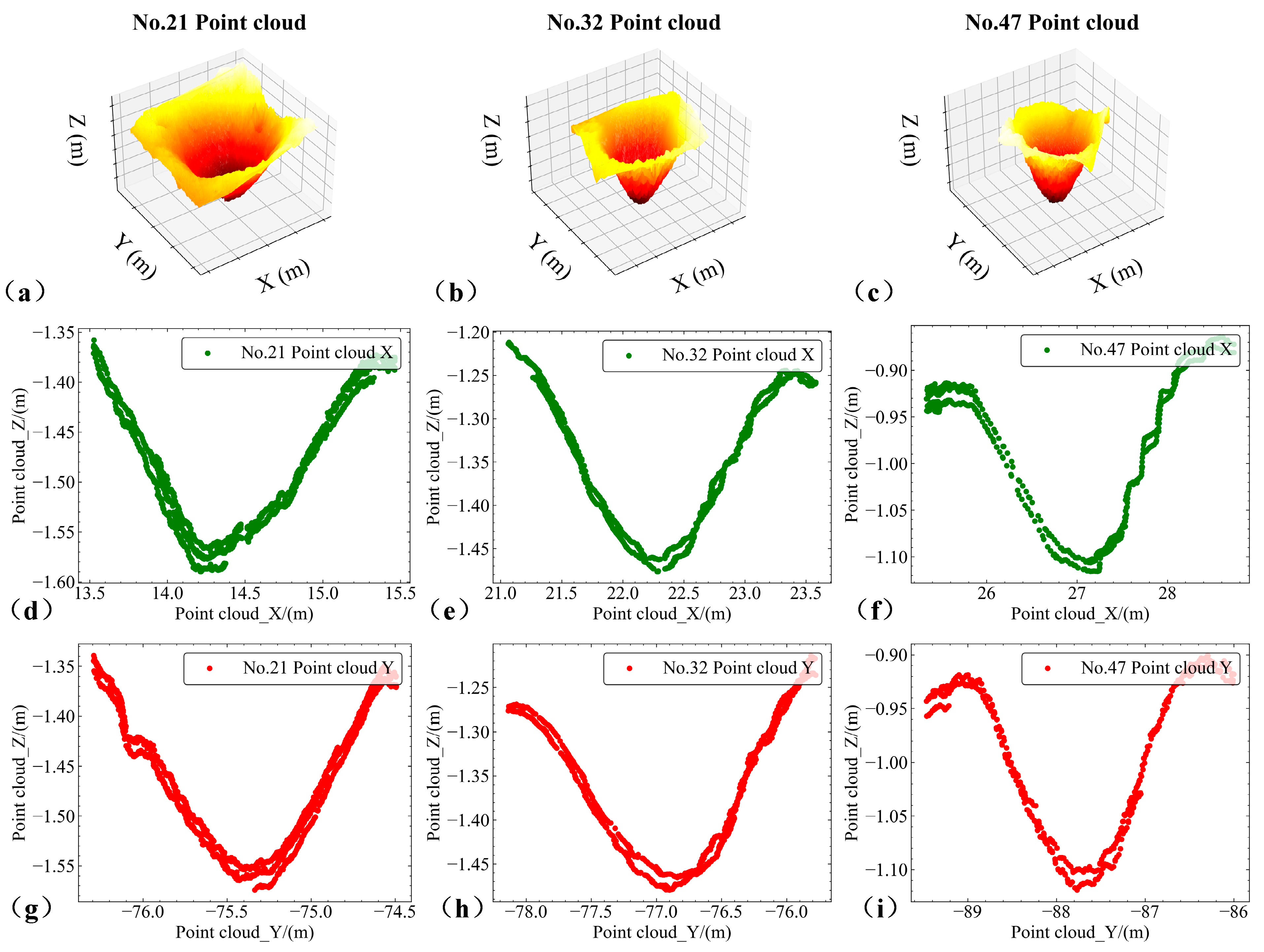
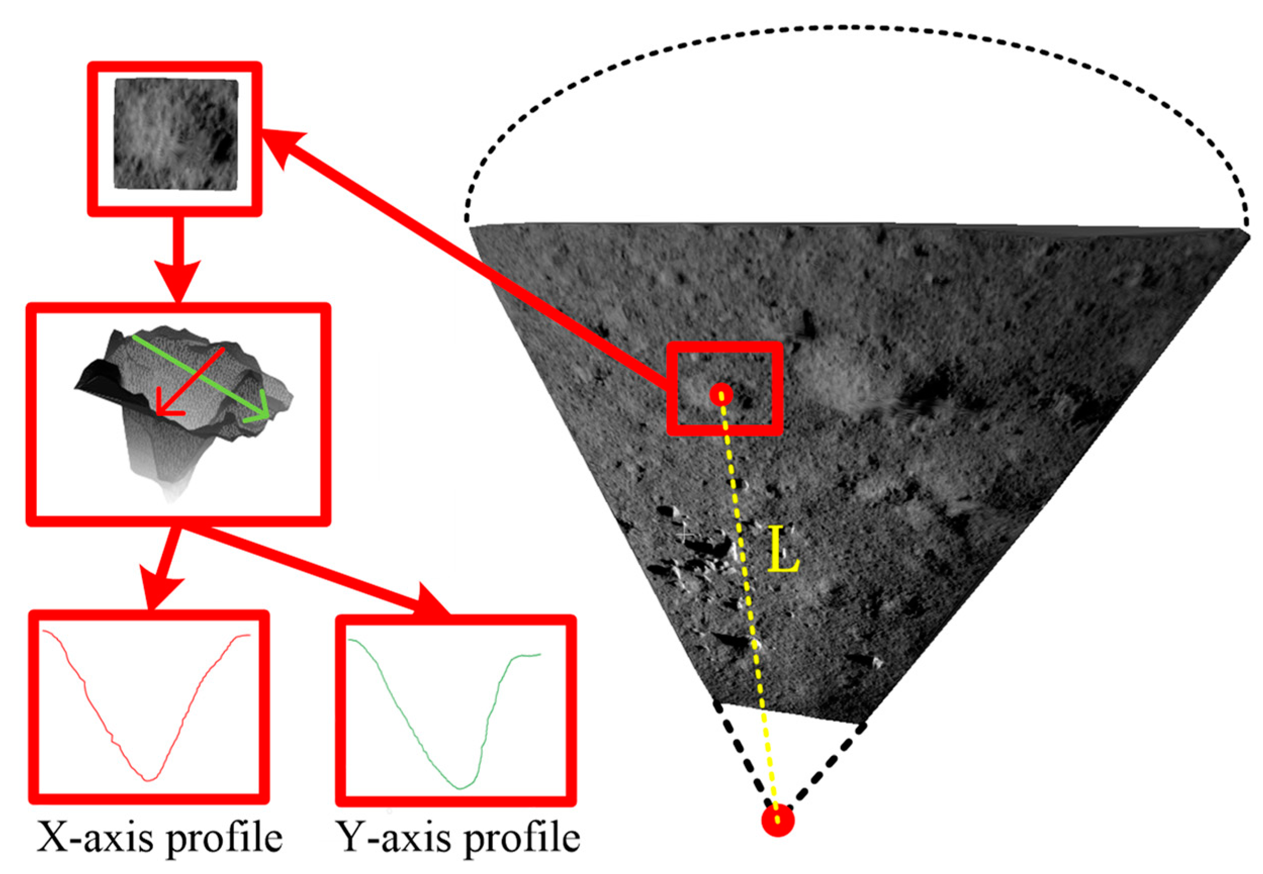
Take the x-axis and y-axis profiles that pass through the lowest point, and project them in the x-axis and y-axis directions to obtain the corresponding contour lines (x-axis and y-axis profiles).

(5)

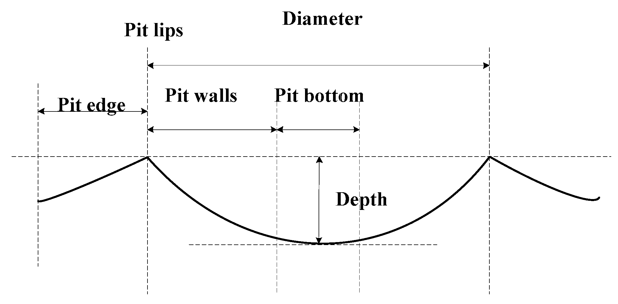
Calculate the diameter of the crater based on the distance between two farthest points on the crater edge.

(6)

Calculate the vertical distance from the lowest point to the line (the line connecting the two points at the crater edge) to obtain the depth of the crater.

3. Experiment and Analysis

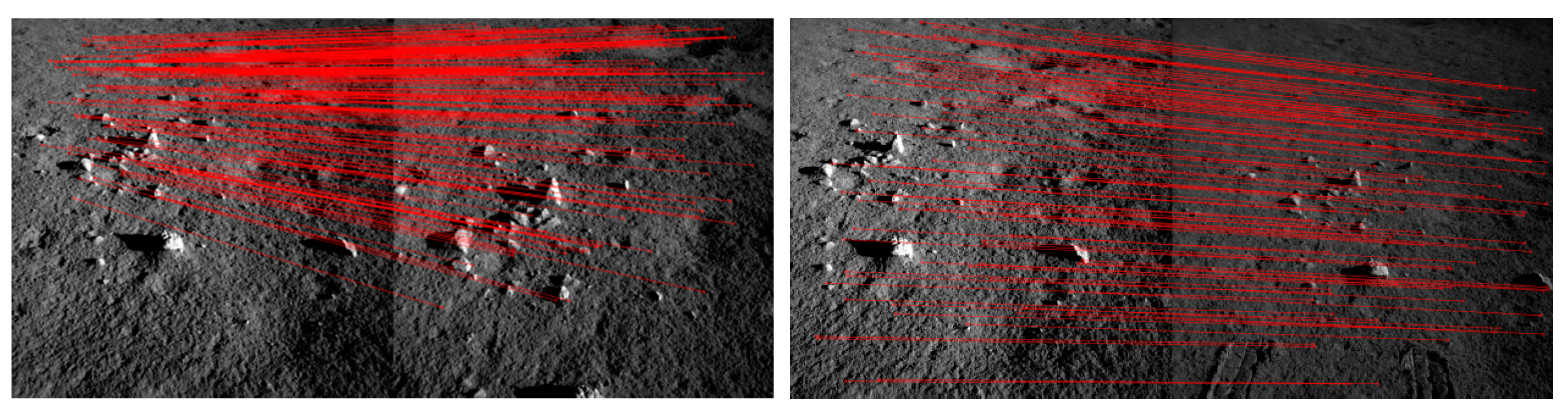
3.1. Experimental Analysis of Stereo Image Matching

To verify the effectiveness of the CscaNet algorithm in sparse texture scenarios, it is tested in a computer environment configured with an NVIDIA 1660S GPU. With the PyTorch deep learning framework, the training sample size is set to 2, the maximum parallax is determined using the Adam optimizer, and the beta parameters are set to (${\beta }_1$ = 0.9, ${\beta }_2$ = 0.999). First, the model network of the CscaNet algorithm is trained on the SceneFlow dataset. The number of epochs in the training process is set to 10, the 3D learning rate for the first eight epochs is set to 0.001, and the learning rate for the remaining epochs is set to 0.0005. Second, transfer learning is performed on the Karlsruhe Institute of Technology and Toyota Technical Institute (KITTI) 2015 dataset using a pre-trained model with the number of epochs set to 300. The learning rate for the first 200 epochs is set to 0.001, the learning rate for the last 100 epochs is set to 0.005, and a weight file is generated. Finally, quantitative and qualitative tests of parallax estimation are performed for CscaNet, GC-Net, DispNet, and PSMNet on the KITTI 2015 dataset, SceneFlow dataset, and lunar surface environment images. The input of this section is a stereo navigation image, the direct output is the corresponding parallax map, and the final output is a 3D point cloud.

3.1.1. Parallax Estimation

The KITTI 2015 dataset contains 200 training image pairs and 200 test image pairs with a resolution of 1242 × 375; moreover, it offers true parallax values of the sparse surfaces acquired with Lidar. There are three accuracy evaluation indicators, namely, D1-bg, D1-fg, and D1-all, which measure the proportions of the predicted error pixels in the background, foreground, and all regions, respectively, in the first image frame.

The SceneFlow dataset is a virtual stereoscopic dataset generated by software rendering that contains 35,454 training image pairs and 4370 test image pairs with a resolution of 960 × 540 and provides the true values of parallax maps. The accuracy evaluation indicator of this dataset is EPE, which measures the endpoint error of all regions. EPE is the average of the Euclidean distance between the predicted value and the true value; the lower the value of EPE, the better the optimization. The formula is as follows:

$$EPE=\frac{1}{N}{\sum }_{\left(x,y\right)\in N}\left|d_{est}\left(x,y\right)-d_{gt}(x,y)\right|$$

(5)

Next, parallax estimations for the CscaNet algorithm, GC-Net, DispNet, PSMNet, and other techniques are performed on public datasets (the KITTI 2015 dataset and SceneFlow dataset) and stereo image pairs captured by the navigation cameras.

(1)

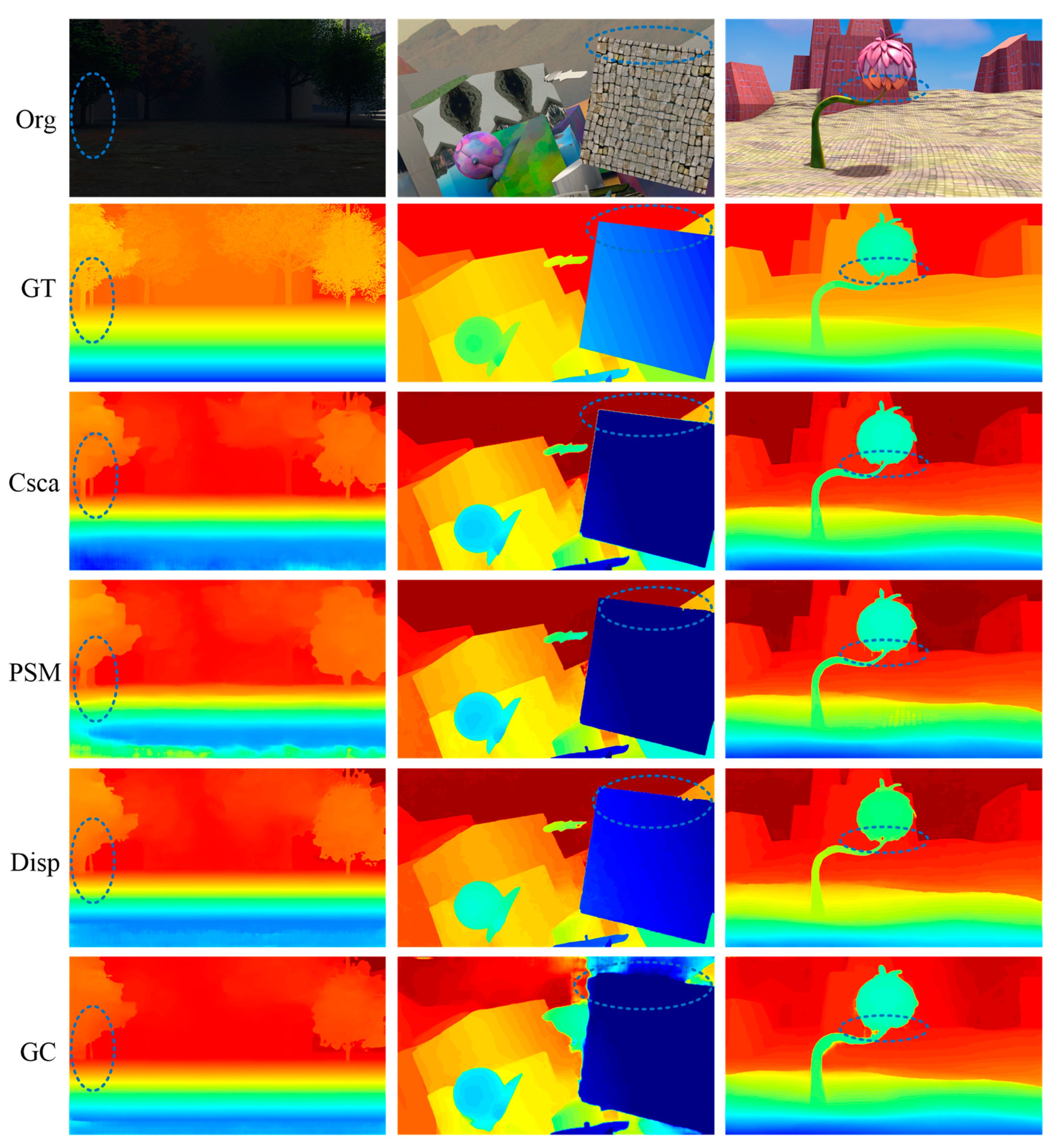
Parallax estimations on public datasets

Figure 14 shows the parallax estimation results of the CscaNet algorithm on the KITTI 2015 dataset; from top to bottom: left images, error graphs, and predicted parallax maps. Figure 15 shows the parallax estimation results of CscaNet on the SceneFlow dataset [42]; from top to bottom: left images, true value graphs, and predicted parallax maps.

As shown in Figure 14 and Figure 15, CscaNet obtains clear feature information from image details in repetitive textured and dim scenes, indicating that the parallax estimation performance of CscaNet is satisfactory.

(2)

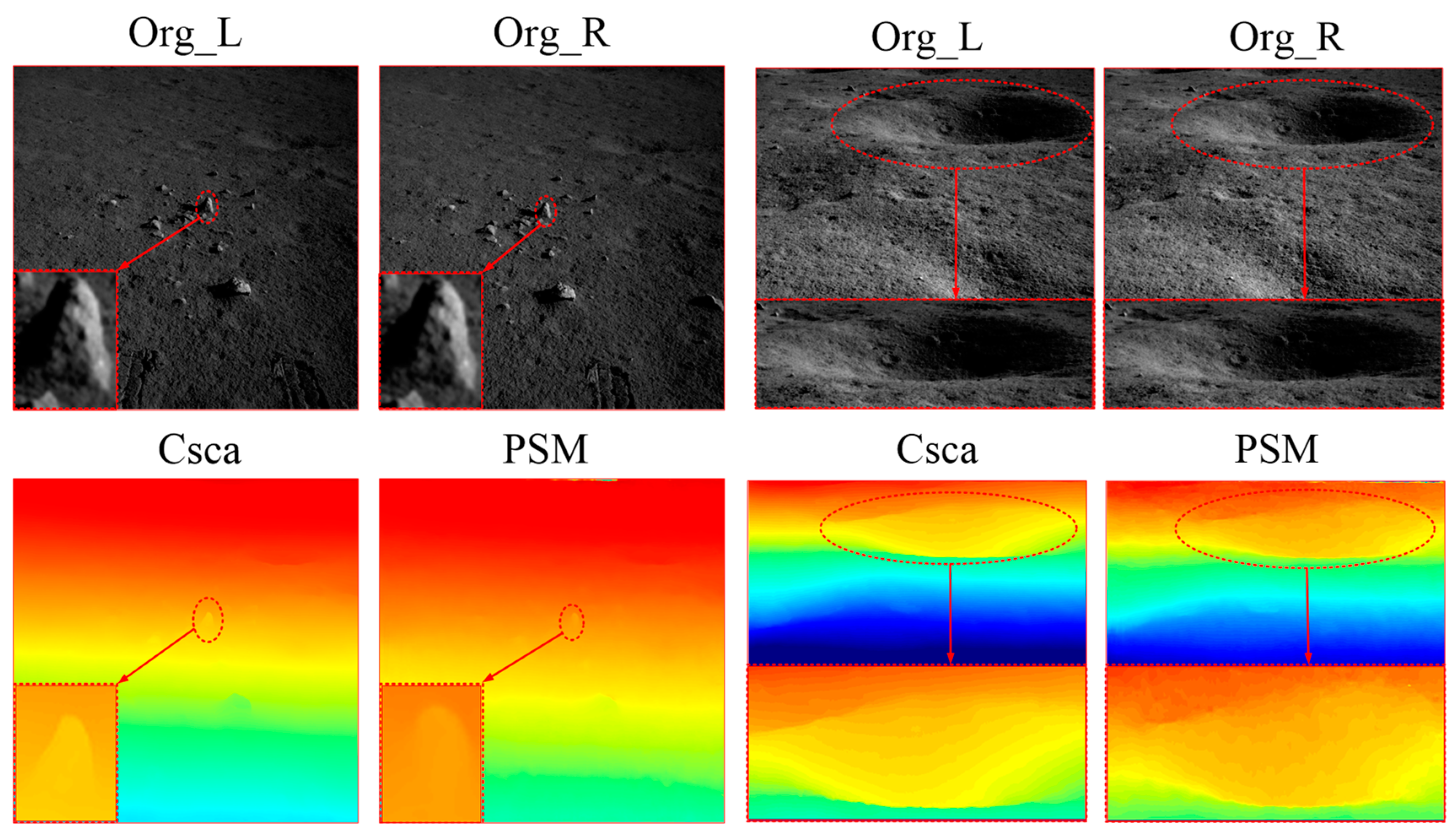
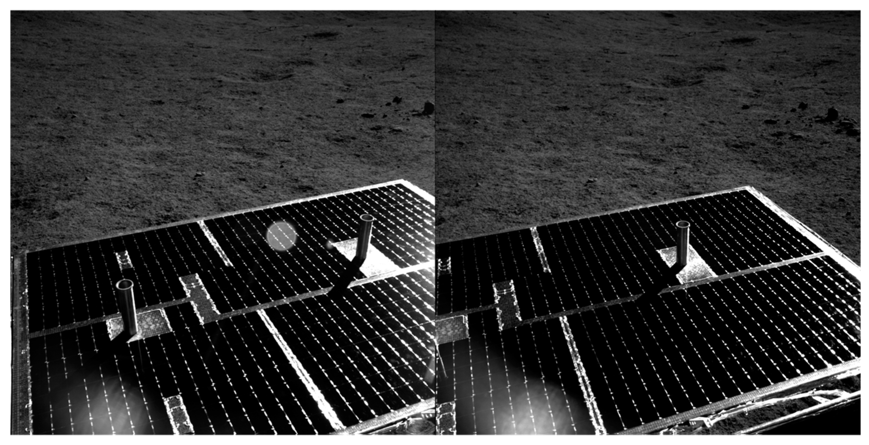
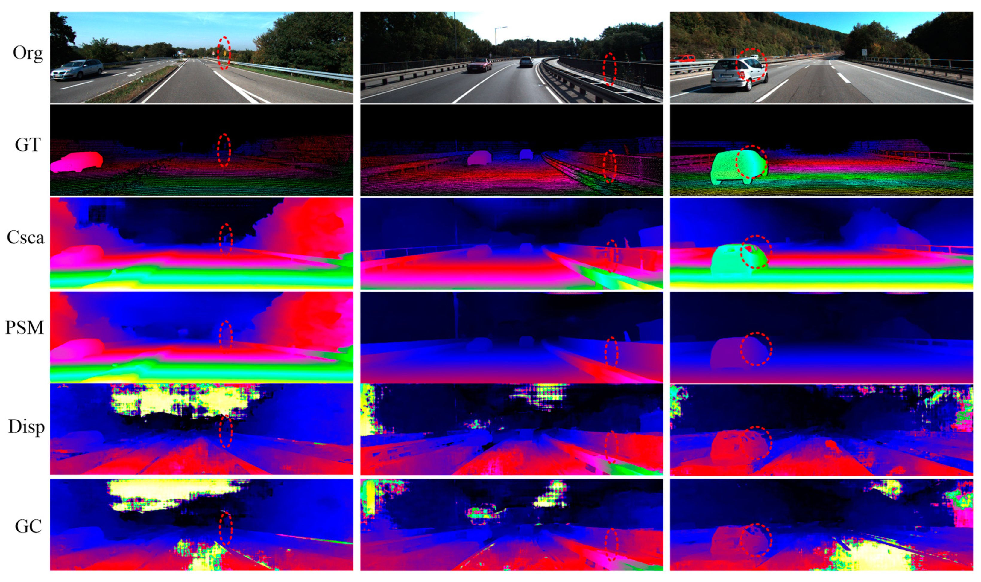
Three-dimensional reconstruction results of stereo navigation images

The stereo navigation images are captured by the Yutu-2 lunar rover at the LE00301-LE00309 exposure stations, totaling 112 pairs. Considering station LE00304 as an example, based on the presence or absence of typical features (craters and rocks), the first and seventeenth stereo image pairs are selected (Figure 16). Due to the lack of real parallax maps for the lunar surface data as quantitative evaluation criteria, the trained weights are used to generate parallax maps for comparison with those generated by PSMNet (Figure 17).

According to Figure 17, the parallax map of the CscaNet is smoother and exhibits the least noise and best matching performance, followed by the PSMNet. To further verify the reconstruction performance for typical features of the lunar surface, 3D point clouds must be generated on the basis of the stereo parallax map. Taking PSMNet and CscaNet as the research objects, CloudCompare software (https://www.cloudcompare.org/, accessed on 15 December 2017) is used to analyze the 3D point clouds of the typical features of the lunar surface generated by the two algorithms. The comparison regions are the red rectangular regions in the first and seventeenth images in Figure 16, where the objects of study are stones and craters; the point cloud size is set to 2, and the local point clouds are shown in Figure 17.

Comparing Figure 17a reveals that the CscaNet algorithm can ensure the reconstruction of the stone point cloud in the illuminated region; the edge reconstruction effect of the stone point cloud in the illuminated region is better than that of the PSMNet. Comparing the red rectangular regions in Figure 17b reveals that the crater edges generated by the CscaNet are more consistent with the actual edge fluctuations than those generated by the PSMNet. The reconstruction results for the typical features (rocks and craters) of the lunar surface obtained using the CscaNet are more consistent with the topography of the actual lunar surface; hence, it is used to recover the 3D point cloud to provide data support for further extraction in the crater experiment.

3.1.2. Performance of CscaNet

In the test on the KITTI 2015 dataset, the improved residual module and the cross-scale cost volume 3D aggregation module proposed for the algorithm of the present study are subjected to hyperparameter analysis. The evaluation metric “D1-all” [43] means the proportion of pixels that are incorrectly predicted in all regions for the first frame, if $\left|d_{est}-d_{gt}\right|<3px or \frac{\left|d_{est}\left(x,y\right)-d_{gt}(x,y)\right|}{d_{gt}}<5\%$ is considered to be correctly estimated, the lower its D1-all value and the better the optimization [43].

The deep convolution kernel size k_s and hyperparameter s determine the performance improvement of the convolution residual module. The EPE values obtained by setting different deep convolution kernel sizes and hyperparameters are shown in Figure 18.

As shown in Figure 18, the EPE value is the largest when the convolution kernel size k_s is 1; because the convolution kernel is small, the residual module cannot extract the feature information effectively. When the convolution kernel size k_s is 5 or 7, the convolution kernel is larger, the complexity of the residual module calculation increases, and overfitting occurs. When the convolution kernel size k_s is 3, the EPE value is the smallest; that is, the module performs best. Hence, the convolution kernel size k_s of the CscaNet algorithm is set to 3. As shown on the right side of Figure 18, the EPE value also gradually increases as the s increases. When the s is 2, the value of EPE is the smallest; thus, the s is set to 2.

The residual module and cost aggregation should be analyzed. The residual module proposed for PSMNet and the residual module with improved convolution proposed in this study are compared with each other. The series cost volume, the joint cost volume, and the cross-scale 3D aggregation module are compared with one another. The comparison is performed on the KITTI 2015 dataset and yields a total of six comparison results, as shown in Table 4.

Table 4 leads to the following conclusions:

(1)

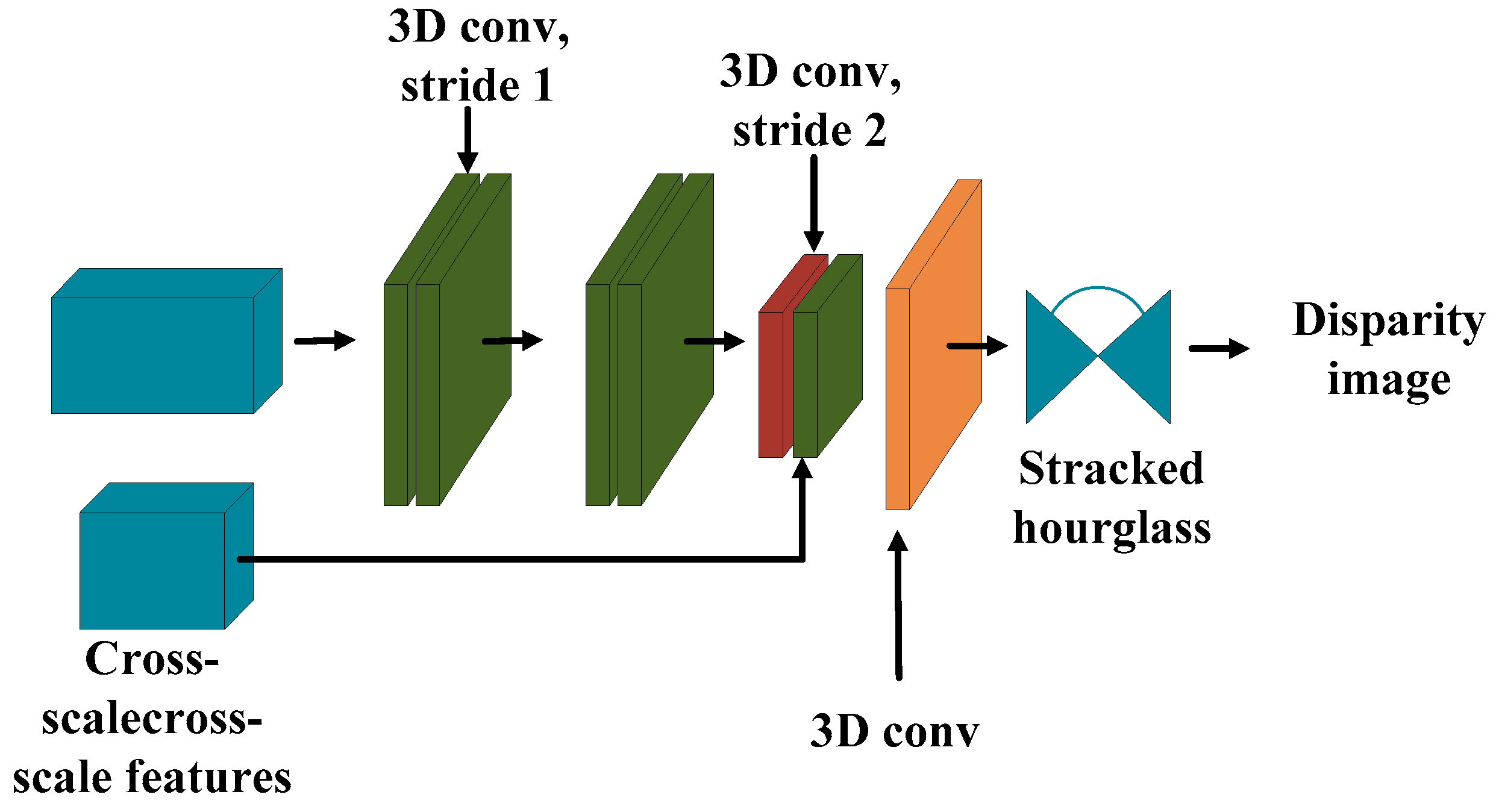
Under the condition that the residual modules are consistent, the effect of the cross-scale 3D aggregation module is better than those of the series cost volume and joint cost volume. With respect to the residual module for PSMNet, the series cost volume, the joint cost volume, and the cross-scale 3D aggregation module are compared with one another; their D1-all are 2.32%, 2.03%, and 1.93%, respectively.

(2)

Under the condition that the cost aggregation modules are consistent, the module with improved convolution is superior to the residual module for PSMNet. In the case of the series cost volume, their D1-alls are 2.32% and 1.87%, respectively. In the case of the joint cost volume, the D1-alls are 2.03% and 1.81%. In the case of the cross-scale 3D aggregation module, the D1-alls are 1.93% and 1.73%, respectively.

According to the results of the experimental analysis, compared with the residual module for PSMNet, the series cost volume, and the joint cost volume, the CscaNet algorithm offers the smallest D1-all and the best parallax estimation performance. Meanwhile, the results in the column “Number of parameters” in Table 4 indicate that the CscaNet algorithm can effectively reduce the number of residual module parameters and 3D hourglass modules [39], thereby reducing the algorithm complexity.

For further evaluation,

Table 5. Performance evaluation of different algorithms on the KITTI 2015 dataset.

Algorithm	Noc (%)			All (%)
	D1-bg	D1-fg	D1-all	D1-bg	D1-fg	D1-all
DispNet	4.11	3.72	4.05	4.32	4.41	4.34
GC-Net	2.02	5.58	2.61	2.21	6.16	2.87
PSMNet	1.71	4.31	2.14	1.86	4.62	2.32
CscaNet	1.59	3.51	1.59	1.25	3.31	1.73

and

Table 6. Performance evaluation of different algorithms on the SceneFlow dataset.

Algorithm	GC-Net	DispNet	PSMNet	CscaNet
EPE	2.51	1.68	1.09	0.74

present the parallax estimation results of the classic algorithms such as CscaNet, GC-Net, DispNet, and PSMNet. In Table 5, “D1” represents the percentage of outliers in terms of pixel error, “All” represents the pixels in all regions, “Noc” denotes the pixels in non-occluded regions, “bg” is the background region, and “fg” is the foreground region. The bolds in Table 5 and Table 6 represent the best performing values.

From Table 5 and Table 6, the following conclusions are drawn: compared with DispNet, GC Net, and PSMNet, the D1-all value for the proposed CscaNet was 1.59% in non-occluded regions and 1.73% in all regions, which surpassed prior studies by a noteworthy margin. The proposed CscaNet also has the best performance in the EPE metric of the SceneFlow dataset.

3.2. Extraction and Analysis of the Metric Features of Craters

This section examines the point clouds of small craters in the Von Karman Crater. First, the crater point cloud was obtained by clipping the point cloud generated by CscaNet. Then, based on the positioning results of the lunar rover, the Euclidean distance L from the center of the crater to the centroid of the lunar rover (L in Figure 19) was determined, and the point cloud was horizontally aligned. Finally, corresponding contour lines were obtained by projection in the x-axis and y-axis directions (x-axis profile and y-axis profile in Figure 19). The input of this section is the trimmed point cloud containing the crater, and the output is the diameter D, depth d, and depth-to-diameter ratio $d_r$ of the crater.

A total of 49 craters were extracted from the 112 pairs of navigation images. The LE00306 station stitched navigation image was used as an example for crater extraction (as shown in Figure 20), and the numbering order was from right to left (from near to far) in front of the lunar rover; the range of the crater from the lunar rover is 0.8–6.1 m and the terrain reconstruction mean accuracy of the crater area is better than 0.98 cm.

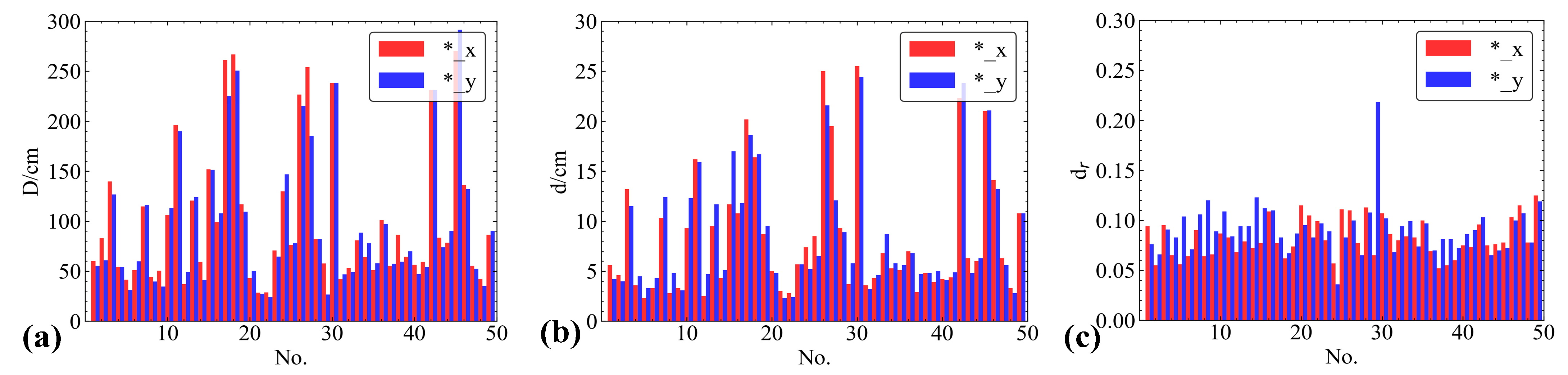
3.2.1. Crater Profile Shape Indicator Statistics

Based on multiple camera stations, stereo image reconstruction was performed to obtain dense point cloud data, and various indicators such as D, d, and $d_r$ from the center of the crater to the center of the lunar vehicle were calculated. In order to visualize the morphological parameters of the craters in a more intuitive and disposable way, we produced statistical histograms, as shown in Figure 21.

Through the statistical analysis of the indicators in Figure 21, the minimum and maximum values of the diameter, depth, and aspect ratio of the crater were obtained. Then, the mean, median, standard deviation, kurtosis, and skewness were calculated using 49 crater indicators, as shown in

Table 7. Parameters of craters.

	Crater Diameter D (cm)	Crater Depth d (cm)	$\mathbf{Depth}–\mathbf{Diameter} \mathbf{Ratio} \mathbf{of} \mathbf{Crater} {\mathit{d}}_{\mathit{r}}$
Minimum	24.3	2.3	0.036
Maximum	291.4	25.5	0.218
Mean	99.7	8.5	0.087
Median	78.5	6.0	0.078
Standard deviation	68.5	6.1	0.023
Kurtosis	0.6	0.9	−0.730
Skewness	1.3	1.3	1.935

.

3.2.2. Analysis of the Correlation and Distribution Relationships of Crater Indicators

The correlation and distribution relationships between the metrics were analyzed using the data above, as shown in Figure 22. The Pearson correlation coefficient (PCC), named after the English mathematician and biostatistician Karl Pearson, is a statistical measure of the degree of linear correlation between two variables. The value of the PCC ranges from −1 to 1, where −1 indicates a complete negative correlation, 0 indicates no linear correlation, and 1 indicates a complete positive correlation.

According to the covariance matrix between the crater diameters of the x-axis profile and the y-axis profile, the PCC can be obtained, ${\eta }_1=0.977$; the PCC of the crater depth between the x-axis profile and the y-axis profile, ${\eta }_2=0.956$; the PCC between the x-axis profile crater depth and crater diameter, ${\eta }_3=0.944$; the PCC between the y-axis profile crater depth and crater diameter, ${\eta }_4=0.930$; the PCC of the crater depth–diameter ratio between the x-axis profile and y-axis profile, ${\eta }_5=0.218$; the PCC between the x-axis profile crater depth–diameter ratio and crater diameter, ${\eta }_6=-0.112$; and the PCC between the y-axis profile crater depth–diameter ratio and crater diameter, ${\eta }_7=-0.172$. Three decimal places were retained for all the results.

From the kurtosis and skewness data in Table 7, it was concluded that the depth, diameter, and depth–diameter ratio values of small craters in this region have small outliers and low dispersion; all the outliers are highly positively skewed. According to Figure 20, the relationships between the diameter and various metrics can be summarized; after analysis, it can be found that the correlations between the diameters and depths of the transverse and longitudinal sections of the craters are high, while the correlations between the depth–diameter ratios are slightly lower. The depth was highly positively correlated with the diameter. With increasing diameter, the depth decreases overall, and the correlation is low. The distributions of crater metrics for craters of less than 1 m in diameter were relatively concentrated, and the distributions of the crater metrics with a diameter greater than 1 m were relatively scattered.

3.3. Geometrical Morphology Analysis of Craters

In reference to the study of Garvin et al. [44], based on the high-precision point cloud and metric distribution law obtained by CscaNet, in order to further analyze how the geometric parameters of craters are related to each other, the present study used the basic expression for the crater shape and the expression in terms of the decimal logarithm to fit the shape parameters of the x-axis profile and y-axis profile of craters in two segments (diameters less than 3 m); calculated the $R^2$ between the function value and the true value after section fitting; and determined its correlation and existence relation. For the x-axis profile and y-axis profile, the overall crater shape parameters were fitted in segments, and the $R^2$ between the function value and the true value after section fitting was determined, along with its correlation and existence relation. The input of this section was the extracted D, d, and d_r and the output is the fitting mathematical relationship of D, d, and d_r.

3.3.1. Morphological Fitting along the X-Axis and Y-Axis Profiles

The data of the $\mathrm{x}$-axis and $\mathrm{y}$-axis profiles were fitted globally, and the results are shown in the figure below:

Based on Figure 23a,b, the expression of the exponential and decimal logarithm was emphasized, and it was found that the PCC between the depth and diameter along the $\mathrm{x}$-axis direction, with ${ R}^2=0.892 \mathrm{a}\mathrm{n}\mathrm{d} 0.877$, respectively, indicated a high degree of fitting. The PCC between the depth and diameter along the $\mathrm{y}$-axis direction, with $R^2=0.866 \mathrm{a}\mathrm{n}\mathrm{d} 0.832$, respectively, indicated a similarly high degree of fitting. According to Figure 23c,d, the PCC between the depth–diameter ratio and diameter along the $\mathrm{x}$-axis direction, with ${ R}^2=0.043 \mathrm{a}\mathrm{n}\mathrm{d} 0.04$, respectively, indicated a lower degree of fitting. The PCC between the depth–diameter ratio and diameter along the $\mathrm{y}$-axis direction, with ${ R}^2=0.001 \mathrm{a}\mathrm{n}\mathrm{d} 0.001$, respectively, indicated a low degree of fitting. Therefore, compared with the high correlation between the depth and diameter, the correlation between the depth–diameter ratio and diameter was weak.

3.3.2. Morphological Fitting along Different Profile Directions and Segments

With a diameter of 1 m as the boundary, segmented and section-specific fittings were performed for the shape parameters of the craters with respect to the $\mathrm{x}$-axis and $\mathrm{y}$-axis profiles to obtain an expression for the logarithmic relationship between the crater depth and diameter, the results are shown in the figure below:

Based on Figure 24a,b, the PCC between the depth and diameter was within the range of less than 1 m, with ${ 0.477\le R}^2\le 0.822$, while the PCC was within the range of greater than 1 m, with ${ 0.594\le R}^2\le 0.632$, indicating a lower fitting degree than the overall fitting. According to Figure 24c,d, the PCC between the depth–diameter ratio and diameter was within the range of less than 1 m, with ${0.001\le R}^2\le 0.183$, while the PCC was within the range of greater than 1 m, with ${ 0.014\le R}^2\le 0.097$, indicating a low fitting degree.

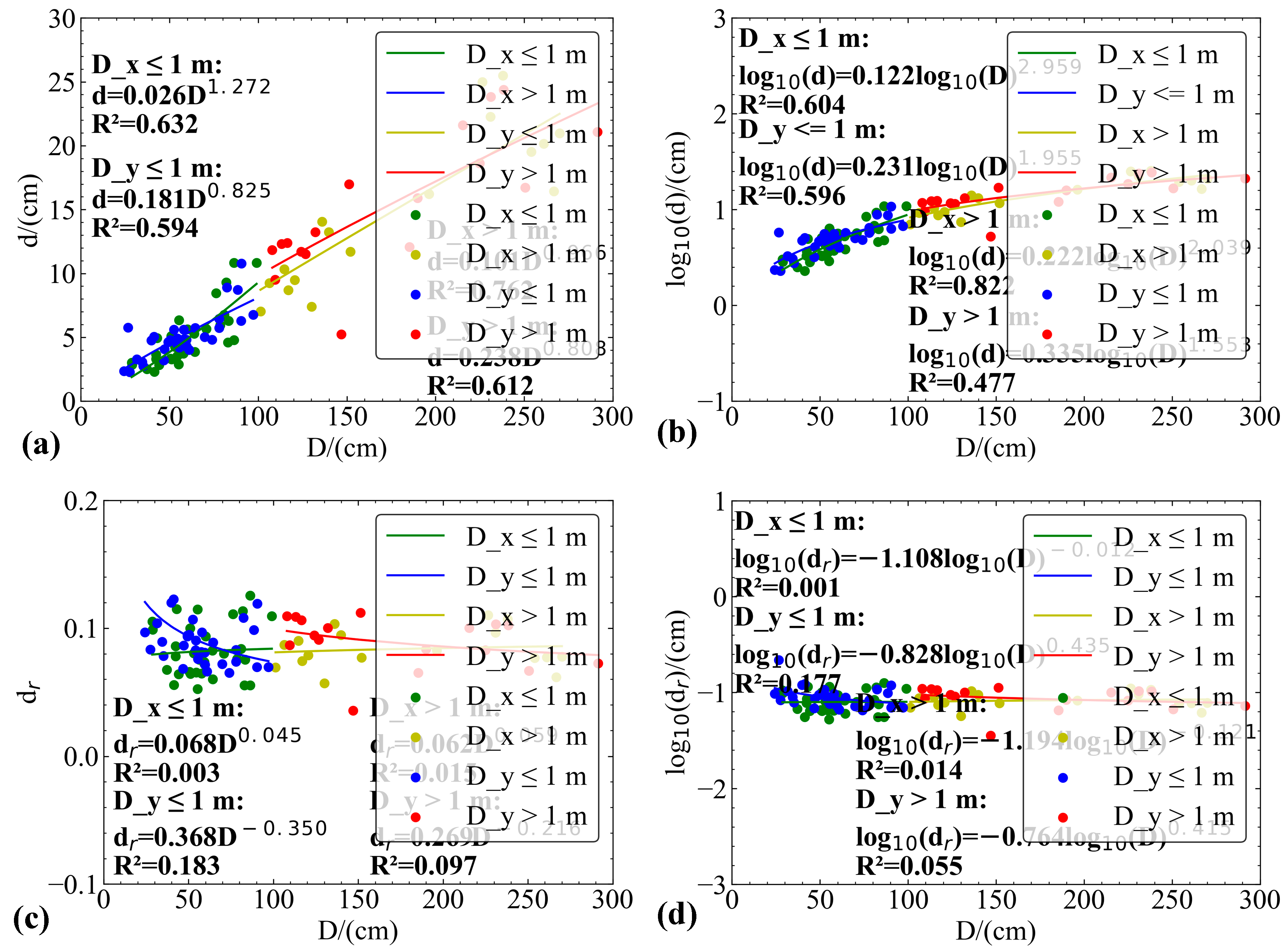
3.3.3. Segmented Fitting by Segmentation

On the basis of the analysis of Figure 22, the relationship between the depth, depth–diameter ratio, and diameter of the segment and the whole was studied without distinguishing the direction of the section, and the fitting result was as follows:

Based on Figure 25a,b, the index expression and decimal logarithmic expression are the key factors in examining the PCC between the depth and diameter for diameters smaller than 1 m, with $R^2=0.591 \mathrm{a}\mathrm{n}\mathrm{d} 0.65$; for diameters larger than 1 m, with $R^2=0.692 \mathrm{a}\mathrm{n}\mathrm{d} 0.756$; and for diameters ranging from 1 m to 3 m, with $R^2=0.895 \mathrm{a}\mathrm{n}\mathrm{d} 0.899$, indicating a higher fitting degree within the 1–3 m diameter range. Based on Figure 25c,d, the $R^2$ between the depth and diameter for diameters smaller than 1 m is $0.071 \mathrm{a}\mathrm{n}\mathrm{d} 0.014,$ respectively; for diameters larger than 1 m, $R^2$ is $0.013 \mathrm{a}\mathrm{n}\mathrm{d} 0.029,$ respectively; and for diameters ranging from 1 m to 3 m, the $R^2$ is $0.001 \mathrm{f}\mathrm{o}\mathrm{r} \mathrm{b}\mathrm{o}\mathrm{t}\mathrm{h}$, indicating a lower fitting degree.

According to the above fitting results, we can obtain the following laws:

(1)

The PCC of the depth–diameter relationship in craters is high, indicating a strong correlation between the two factors.

(2)

The PCC of the depth–diameter ratio and diameter relationship in craters is low, indicating a weak correlation and an underfitting function expression.

(3)

Compared to exponential fitting, logarithmic fitting shows a higher PCC and a smoother curve.

4. Discussion

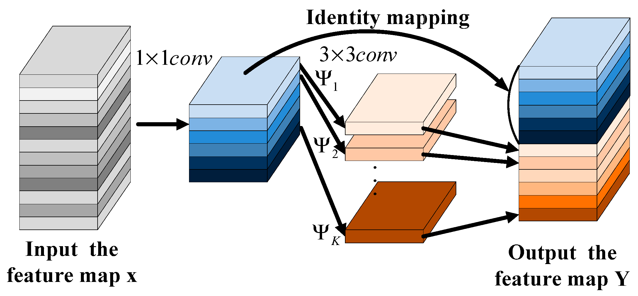
• The features extracted through traditional neural networks are relatively few, especially in the case of special texture features in lunar navigation images. We used deep convolution to complete the training task, which can obtain more redundant features in the feature map, ensuring that the image feature information is expanded and more internal features are extracted and providing more sufficient starting data for subsequent matching.
• Adopting an improved residual module network structure, cascading operations were carried out between different low-level internal features and using the upper level as prior information to further improve the performance of feature extraction. The fusion of low-level internal features and high-level semantic information made the image features more complete and better preserved the detailed information of the extracted image feature maps. It is more helpful for extracting detailed features of navigation images in lunar scenes.
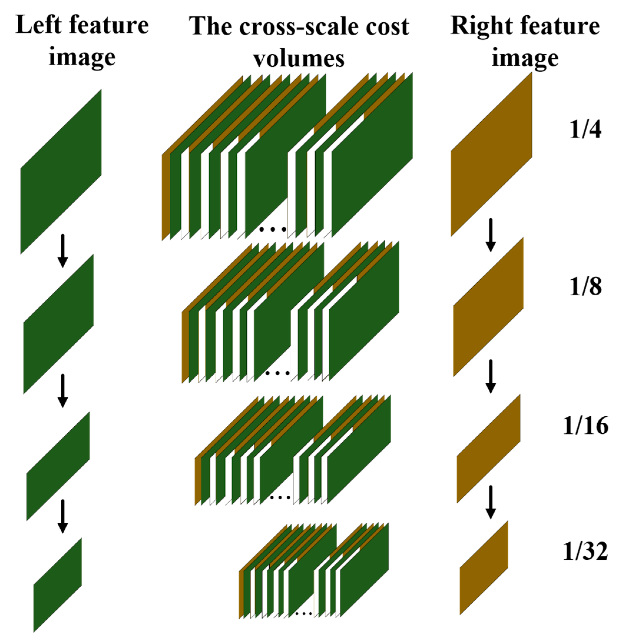
• The proposed method constructs a multi-scale cost volume, taking into account multi-scale spatial relationships, and uses four scale feature maps for multi-scale feature information extraction. The feature information of different scales is extracted at different levels of the spatial feature map, and the above level is used as prior knowledge. After up-sampling to the same scale, the previous scale information is used as prior knowledge for cascading operations, which can provide a more accurate, more complete similarity measurement and global context information. Due to the different matching costs at different scales, the final cost obtained by using small scales as prior knowledge is more accurate in matching the results.
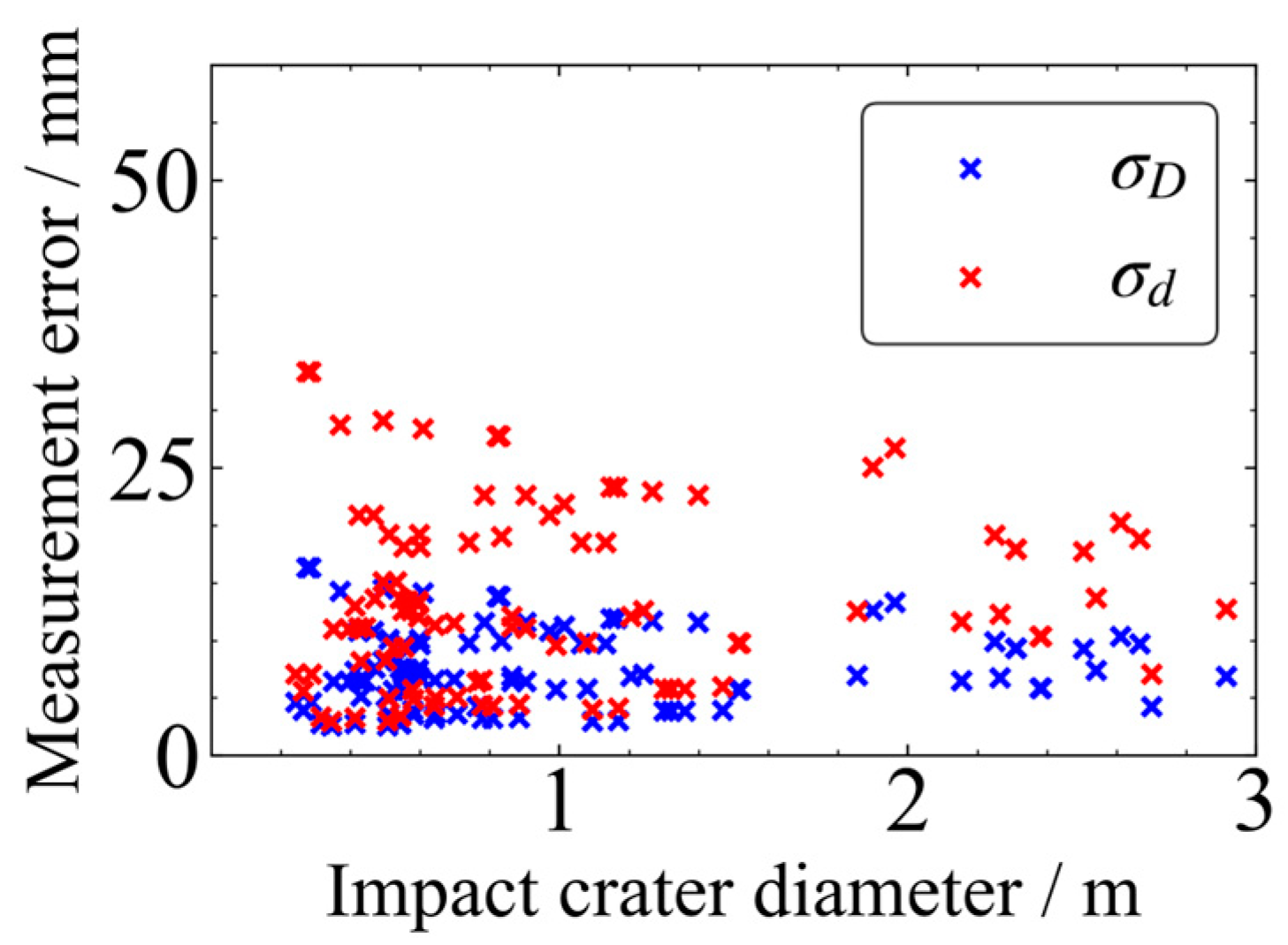
• The average error in diameter caused by the 3D reconstruction results is 7 mm and the average error in depth is 13 mm, which fully demonstrates that the extraction of crater diameter and depth indicators in this paper is reliable.
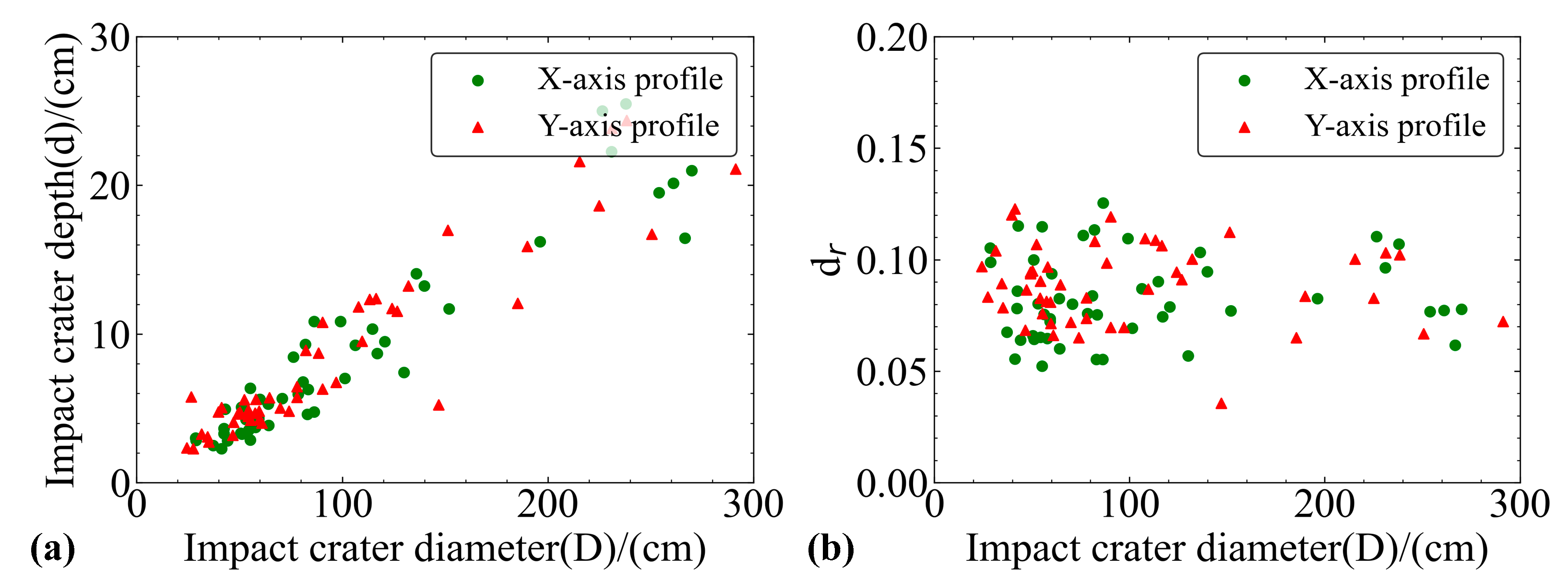
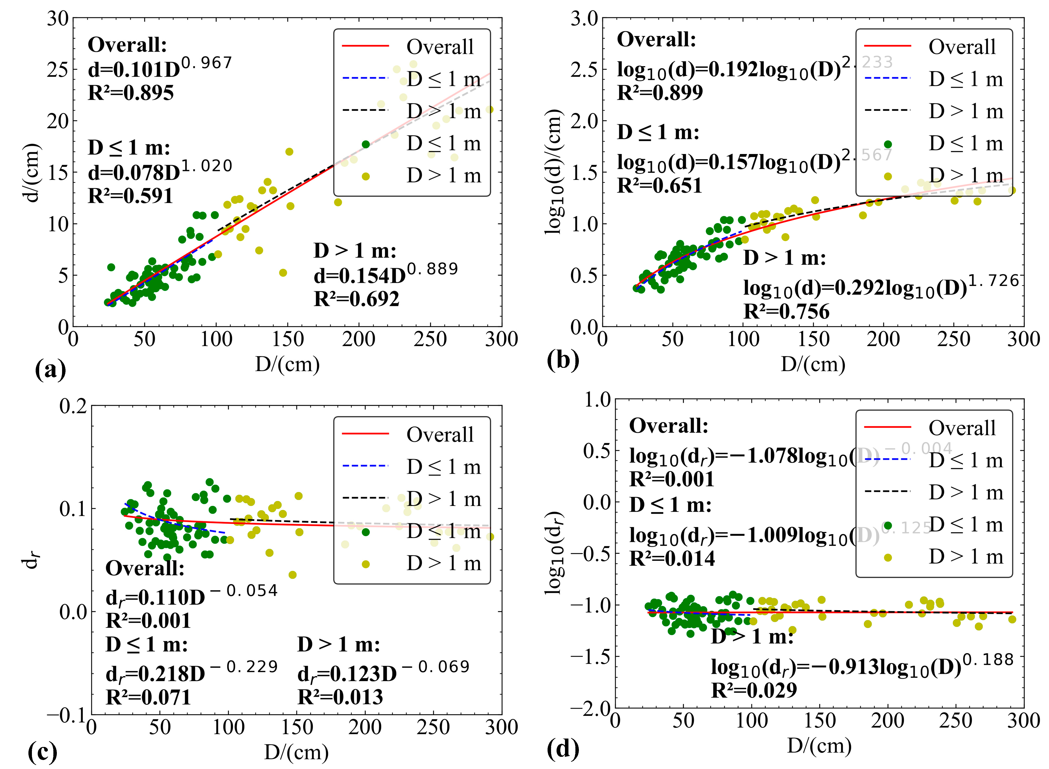
• The law between the D and dr of small craters (diameter < 3 m) was analyzed, and the degree of steepness of small craters is inversely proportional to their D. As the D increases, dr decreases. The mathematical expression ${log}_{10}\left(d\right)=-1.078{{log}_{10}\left(D\right)}^{-0.004}$ of the two has a correlation coefficient of only ${ R}^2=0.001$, indicating a small correlation between the two. The mathematical expression indicates that the surface between the two appears to conform to a certain trend but cannot be better fitted.
• As the D increases, d also increases, and there is a positive correlation between the two. The mathematical expression obtained by fitting D and d has a higher correlation coefficient and a better correlation.
• The obtained expression is different from the results of other scholars. The 3D reconstruction of high-precision small craters can have higher accuracy, and the fitting results are reliable, indicating that there may be significant differences in the formation and evolution process of small craters compared to large craters (with a diameter greater than 3 m). In addition, it can provide better data support for other scholars in studying lunar soil composition, lunar evolution, and other processes.

5. Conclusions

We implemented 3D reconstruction of small craters using the proposed CscaNet based on stereo navigation images and extracted three typical geometric indicators of craters, namely, D, d, and d_r. The geometric shape of the craters was analyzed, and the following conclusions were obtained:

(1)

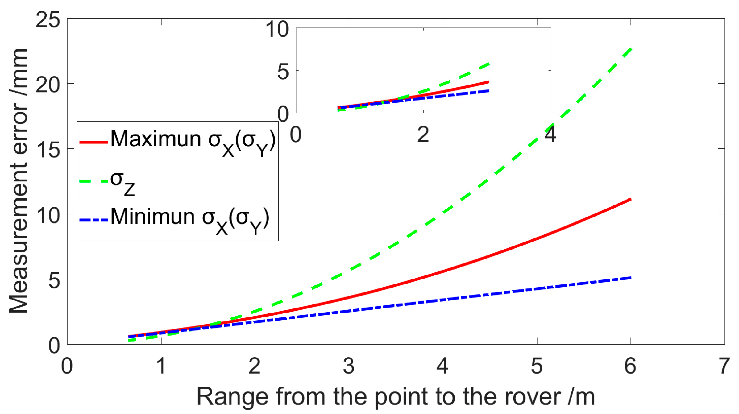
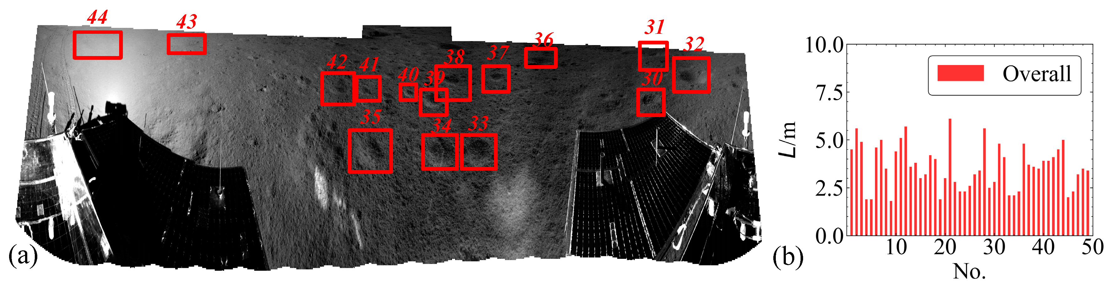
The reconstruction accuracy of the proposed CscaNet is superior to GC-Net, DispNet, and PSMnet. The reconstruction accuracy is better than 0.98 cm within the range of 0.8–6.1 m between the crater and the lunar rover.

(2)

When the diameter is less than 1 m, the depth and diameter indicators of the crater are relatively concentrated. When the diameter is less than 3 m, there is a significant difference in the shape of the crater, and the distribution of the depth and diameter indicators is relatively discrete.

(3)

Quantitative fitting was conducted, and the relationship between d and D was obtained: ${log}_{10}(d)=0.192{{log}_{10}\left(D\right)}^{2.233}$ or $d=0.101D^{0.967}$. However, the correlation between d_r and d is low and it is not suitable for expressing the morphology of small craters.

The geometrical morphology analysis of small craters in the Von Karman Crater of the SPA Basin will provide data support for subsequent studies on the evolution of degradation on the far side of the Moon and navigation planning for lunar rovers.

References

- Breccia, L. A breccia is a rock that is composed of other rock fragments. On the lunar surface, the main process for fragmentation is meteorite impacts. J. Am. Assoc. Adv. Sci. 2023, 8, 26. [Google Scholar]
- Ping, J.; Huang, Q.; Yan, J.; Meng, Z.; Wang, M. A Hidden Lunar Mascon Under the South Part of Von Kármán Crater. J. Deep. Space Explor. 2018, 5, 34–40. [Google Scholar]
- Head, J.W. Origin of central peaks and peak rings: Evidence from peak-ring basins on Moon, Mars, and Mercury. In Proceedings of the 9th Lunar and Planetary Science Conference, Houston, TX, USA, 13–17 March 1978; pp. 485–487. [Google Scholar]
- Head, J.W., III; Fassett, C.I.; Kadish, S.J.; Smith, D.E.; Zuber, M.T.; Neumann, G.A.; Mazarico, E. Global distribution of large lunar craters: Implications for resurfacing and impactor populations. Science 2010, 329, 1504–1507. [Google Scholar] [CrossRef]
- Kadish, S.J.; Fassett, C.I.; Head, J.W.; Smith, D.E.; Zuber, M.T.; Neumann, G.A.; Mazarico, E. A global catalog of large lunar craters (≥20 km) from the Lunar Orbiter Laser Altimeter. In Proceedings of the 42nd Annual Lunar and Planetary Science Conference, The Woodlands, TX, USA, 7–11 March 2011; p. 1006. [Google Scholar]
- McDowell, J. A Merge of a Digital Version of the List of Lunar Craters from Andersson and Whitaker with the List from the USGS Site. Available online: http://www.planet4589.org/astro/lunar/CratersS (accessed on 24 June 2023).
- Salamunićcar, G.; Lončarić, S.; Mazarico, E. LU60645GT and MA132843GT catalogues of Lunar and Martian craters developed using a Crater Shape-based interpolation crater detection algorithm for topography data. Planet. Space Sci. 2012, 60, 236–247. [Google Scholar] [CrossRef]
- Robbins, S.J. A New Global Database of Lunar Craters >1–2 km: 1. Crater Locations and Sizes, Comparisons With Published Databases, and Global Analysis. J. Geophys. Res. Planets 2018, 124, 871–892. [Google Scholar] [CrossRef]
- Robbins, S.J.; Antonenko, I.; Kirchoff, M.R.; Chapman, C.R.; Fassett, C.I.; Herrick, R.R.; Singer, K.; Zanetti, M.; Lehan, C.; Huang, D.; et al. The variability of crater identification among expert and community crater analysts. Icarus 2014, 234, 109–131. [Google Scholar] [CrossRef]
- Wang, J.; Zhou, C.; Cheng, W. The Spatial Pattern of Lunar Craters on a Global Scale. Geomat. Inf. Sci. Wuhan Univ. 2017, 42, 512–519. [Google Scholar]
- Hou, L. Spatial Distribution and Morphology Characteristics Quantitative Description of the Lunar Craters. Master’s Thesis, Northeast Normal University, Changchun, China, 2013. [Google Scholar]
- Li, K. Study on Small-Scale Lunar Craters’ Morphology and Degradation. Ph.D. Thesis, Wuhan University, Wuhan, China, 2013. [Google Scholar]
- Zhao, D. Intelligent Identification and Spatial Distribution Analysis of Small Craters in Lunar Landing Area. Master’s Thesis, Jilin University, Jilin, China, 2022. [Google Scholar]
- Zuo, W.; Li, C.; Yu, L.; Zhang, Z.; Wang, R.; Zeng, X.; Liu, Y.; Xiong, Y. Shadow–highlight feature matching automatic small crater recognition using high-resolution digital orthophoto map from Chang’E Missions. Acta Geochim. 2019, 38, 541–554. [Google Scholar] [CrossRef]
- Hu, Y.; Xiao, J.; Liu, L.; Zhang, L.; Wang, Y. Detection of Small Craters via Semantic Segmenting Lunar Point Clouds Using Deep Learning Network. Remote Sens. 2021, 13, 1826. [Google Scholar] [CrossRef]
- Kang, Z.; Wang, X.; Hu, T.; Yang, J. Coarse-to-fine extraction of small-scale lunar craters from the CCD images of the Chang’E lunar orbiters. IEEE Trans. Geosci. Remote Sens. 2018, 57, 181–193. [Google Scholar] [CrossRef]
- Yang, H.; Xu, X.; Ma, Y.; Xu, Y.; Liu, S. CraterDANet: A Convolutional Neural Network for Small-Scale Crater Detection via Synthetic-to-Real Domain Adaptation. IEEE Trans. Geosci. Remote Sens. 2022, 60, 4600712. [Google Scholar] [CrossRef]
- Heiken, G.; Vaniman, D.; French, B.M. Lunar Sourcebook—A User’s Guide to the Moon; Cambridge University Press: Cambridge, UK, 1991; 753 p. [Google Scholar]
- Bouška, J. Crater Diameter–Depth Relationship from Ranger Lunar Photographs. Nature 1967, 213, 166. [Google Scholar] [CrossRef]
- Pike, R.J.; Spudis, P.D. Basin-ring spacing on the Moon, Mercury, and Mars. Earth Moon Planets 1987, 39, 129–194. [Google Scholar] [CrossRef]
- Pike, R.J. Craters on Earth, Moon, and Mars: Multivariate classification and mode of origin. Earth Planet. Sci. Lett. 1974, 22, 245–255. [Google Scholar] [CrossRef]
- Cintala, M.J.; Head, J.W.; Mutch, T.A. Martian crater depth/diameter relationships-Comparison with the moon and Mercury. In Proceedings of the 7th Lunar and Planetary Science Conference Proceedings, Houston, TX, USA, 15–19 March 1976; pp. 3575–3587. [Google Scholar]
- Hale, W.S.; Grieve, R.A.F. Volumetric analysis of complex lunar craters: Implications for basin ring formation. J. Geophys. Res. Solid Earth 1982, 87, A65–A76. [Google Scholar] [CrossRef]
- Croft, S.K. Lunar crater volumes-Interpretation by models of cratering and upper crustal structure. In Proceedings of the 9th Lunar and Planetary Science Conference Proceedings, Houston, TX, USA, 13–17 March 1978; pp. 3711–3733. [Google Scholar]
- Hu, H.; Yang, R.; Huang, D.; Yu, B. Analysis of depth-diameter relationship of craters around oceanus procellarum area. J. Earth Sci. 2010, 21, 284–289. [Google Scholar] [CrossRef]
- Zhang, S.; Liu, S.; Ma, Y.; Qi, C.; Ma, H.; Yang, H. Self calibration of the stereo vision system of the Chang’e-3 lunar rover based on the bundle block adjustment. ISPRS J. Photogramm. Remote Sens. 2017, 128, 287–297. [Google Scholar] [CrossRef]
- Xu, X.; Liu, M.; Peng, S.; Ma, Y.; Zhao, H.; Xu, A. An In-Orbit Stereo Navigation Camera Self-Calibration Method for Planetary Rovers with Multiple Constraints. Remote Sens. 2022, 14, 402. [Google Scholar] [CrossRef]
- Yan, Y.; Peng, S.; Ma, Y.; Zhang, S.; Qi, C.; Wen, B.; Li, H.; Jia, Y.; Liu, S. A calibration method for navigation cameras’ parameters of planetary detector after landing. Acta Geod. Cartogr. Sin. 2022, 51, 437–445. [Google Scholar]
- Wang, B.; Zhou, J.; Tang, G.; Di, K.; Wan, W.; Liu, C.; Wang, Z. Research on visual localization method of lunar rover. Sci. China Inf. Sci. 2014, 44, 452–460. [Google Scholar]
- Liu, C.; Tang, G.; Wang, B.; Wang, J. Integrated INS and Vision-Based Orientation Determination and Positioning of CE-3 Lunar Rover. J. Spacecr. TT C Technol. 2014, 33, 250–257. [Google Scholar]
- Ma, Y.; Peng, S.; Zhang, J.; Wen, B.; Jin, S.; Jia, Y.; Xu, X.; Zhang, S.; Yan, Y.; Wu, Y.; et al. Precise visual localization and terrain reconstruction for China’s Zhurong Mars rover on orbit. Chin. Sci. Bull. 2022, 67, 2790–2801. [Google Scholar] [CrossRef]
- Li, M.; Liu, S.; Peng, S.; Ma, Y. Improved Dynamic Programming in the Lunar Terrain Reconstruction. Opto-Electron. Eng. 2013, 40, 6–11. [Google Scholar]
- Cao, F.; Wang, R. Stereo matching algorithm for lunar rover vision system. J. Jilin Univ. (Eng. Technol. Ed.) 2011, 41, 24–28. [Google Scholar]
- Qi, N.; Hou, J.; Zhang, H. Stereo Matching Algorithm for Lunar Rover. J. Nanjing Univ. Sci. Technol. 2008, 159, 176–180. [Google Scholar]
- Peng, M.; Di, K.; Liu, Z. Adaptive Markov random field model for dense matchingof deep space stereo images. J. Remote Sens. 2014, 18, 77–89. [Google Scholar]
- Zbontar, J.; LeCun, Y. Stereo matching by training a convolutional neural network to compare image patches. J. Mach. Learn. Res. 2016, 17, 2287–2318. [Google Scholar]
- Mayer, N.; Ilg, E.; Hausser, P.; Fischer, P.; Cremers, D.; Dosovitskiy, A.; Brox, T. A large dataset to train convolutional networks for disparity, optical flow, and scene flow estimation. In Proceedings of the IEEE Conference on Computer Vision and Pattern Recognition, Las Vegas, NV, USA, 27–30 June 2016; pp. 4040–4048. [Google Scholar]
- Kendall, A.; Martirosyan, H.; Dasgupta, S.; Henry, P.; Kennedy, R.; Bachrach, A.; Bry, A. End-to-end learning of geometry and context for deep stereo regression. In Proceedings of the IEEE International Conference on Computer Vision, Honolulu, HI, USA, 21–26 July 2017; pp. 66–75. [Google Scholar]
- Chang, J.R.; Chen, Y.S. Pyramid stereo matching network. In Proceedings of the IEEE Conference on Computer Vision and Pattern Recognition, Salt Lake City, UT, USA, 18–23 June 2018; pp. 5410–5418. [Google Scholar]
- Ma, Y.; Liu, S.; Bing, S.; Wen, B.; Peng, S. A precise visual localisation method for the chinese chang’e-4 Yutu-2 rover. Photogramm. Rec. 2020, 35, 10–39. [Google Scholar] [CrossRef]
- Bay, H.; Ess, A.; Tuytelaars, T.; Van Gool, L. Speeded-up robust features (SURF). Comput. Vis. Image Underst. 2008, 110, 346–359. [Google Scholar] [CrossRef]
- Menze, M.; Geiger, A. Object scene flow for autonomous vehicles. In Proceedings of the IEEE Conference on Computer Vision and Pattern Recognition, Boston, MA, USA, 7–12 June 2015; pp. 3061–3070. [Google Scholar]
- Xu, B.; Xu, Y.; Yang, X.; Jia, W.; Guo, Y. Bilateral grid learning for stereo matching networks. In Proceedings of the IEEE/CVF Conference on Computer Vision and Pattern Recognition, Nashville, TN, USA, 20–25 June 2021; pp. 12497–12506. [Google Scholar]
- Garvin, J.B.; Frawley, J.J. Geometric properties of Martian craters: Preliminary results from the Mars Orbiter Laser Altimeter. Geophys. Res. Lett. 1998, 25, 4405–4408. [Google Scholar] [CrossRef]