CE-RX: A Collaborative Cloud-Edge Anomaly Detection Approach for Hyperspectral Images

Abstract

Due to the constrained processing capabilities of real-time detection techniques in remote sensing applications, it is often difficult to obtain detection results with high accuracy in practice. To address this problem, we introduce a new real-time anomaly detection algorithm for hyperspectral images called cloud–edge RX (CE-RX). The algorithm combines the advantages of cloud and edge computing. During the data acquisition process, the edge performs real-time detection on the data just captured to obtain a coarse result and find the suspicious anomalies. At regular intervals, the suspicious anomalies are sent to the cloud for further detection with a highly accurate algorithm, then the cloud sends back the (high-accuracy) results to the edge for information updating. After receiving the results from the cloud, the edge updates the information of the detector in the real-time algorithm to improve the detection accuracy of the next acquired piece of data. Our experimental results demonstrate that the proposed cloud–edge collaborative algorithm can obtain more accurate results than existing real-time detection algorithms.

1. Introduction

With the advance of spectral imaging technologies and the subsequent improvement of spectral resolution, hyperspectral remote sensing data now provides extremely detailed information for earth observation [1,2,3,4]. Hyperspectral target detection [5,6,7,8,9,10] is one of the most important research directions in hyperspectral image processing. It utilizes the rich spectral information contained in hyperspectral images to effectively separate targets from background pixels. However, in practical situations, it is difficult to obtain labeled sample data [11,12,13]. Therefore, anomaly detection (an unsupervised approach to detect targets) has a wider practical application.

Anomaly detection can be considered a binary problem. The anomaly detection algorithm extracts information based on the principle that the features of anomalies and background are different [14,15,16]. A hyperspectral image is divided into background pixels and anomalies during the detection process. The RX detection algorithm proposed by Reed and Xiaoli [17,18] is considered the benchmark anomaly detection algorithm. This algorithm first calculates the Mahalanobis distance between the current pixel and the mean value of the background data. Then, the RX detection algorithm determines whether the current pixel is an anomalous pixel based on the magnitude of the distance. Nowadays, different algorithms have been proposed to improve detection accuracy. Li et al. present a new hyperspectral anomaly detection baseline network, referred to as LRR-Net [19], which synergizes the low-rank representation model with deep learning (DL) techniques. Gao et al. proposed a novel chessboard topology-based anomaly detection (CTAD) method to adaptively dissect images and extract detailed information about land cover [20]. In [21], Wang proposed a joint anomaly detection and noise removal paradigm called DSR-ADNR. This algorithm develops a double subspace representation method to obtain both denoised and detection results simultaneously.

However, these anomaly detection algorithms need to wait for the spectrometer to capture all the image data before obtaining the result. In other words, they output all the detection results at once. These algorithms cannot detect anomalies in real time. Real-time processing is very important in the field of hyperspectral imaging [22,23,24], especially for hyperspectral anomaly detection. In order to cope with the demand for real-time detection, different algorithms have been recently proposed to improve the speed of the detection algorithm. Du proposed a fast CLDA detection classification algorithm for target detection and classification [25]. Chang proposed an LCMV-based target detector. This detector can be processed line-by-line in real time [26]. Zhao [27] proposed a real-time RX detection algorithm that uses Woodbury’s lemma to simplify the calculation of each detection step. This method allows us to quickly achieve detection results without the need to collect the full image data. Chen found the real-time causal version of R-RXD [28,29]. Zhao [30] combined the kernel collaborative representation detector (KCRD) and Cholesky decomposition to propose a real-time version called RT-KCRD.

A real-time process must be causal in the sense that no data sample vectors beyond the current data sample vector being processed should be allowed to be included in the data processing. Existing real-time algorithms are designed based on the principle of using the currently captured data to construct detection operators. When executing these algorithms, the information used comes from the hyperspectral data already captured. Real-time algorithms often suffer from low detection accuracy compared to standard algorithms that can process the entire area data, especially at the initial detection stage. Due to the small amount of data captured by edge devices, real-time algorithms are often unable to accurately detect anomalies and separate them from the background pixels. The inability to execute accurate background suppression at the previous detection stage will negatively affect the subsequent results and will ultimately reduce the overall detection accuracy.

The edge can collect the data faster than the cloud to obtain a real-time result [31,32,33]. However, limited by the performance of the edge devices, the real-time algorithm cannot correct the previous inaccuracy detection results and affects the subsequent detection results. In general, the cloud has a huge amount of computing resources that allow us to process a large number of computation tasks simultaneously and obtain high-accuracy results [34,35,36]. However, it needs to wait for a while before the latest data can be uploaded to the cloud for computation. The data needs to be transferred to the cloud before the detection algorithm can be executed. The cloud can perform fast calculations, but the latency of data transmission prevents the cloud from capturing data and performing real-time inspections at the same time.

Nowadays, cloud–edge computing technology has been widely used in many fields. The most common model is that the edge offloads part of the computational tasks to the cloud. The edge and the cloud accomplish a computational task together [35,37,38]. In the literature [39,40], people deploy a complex algorithm in the cloud and deploy a simple algorithm at the edge. When the algorithms at the edge cannot meet the computational requirements, the data are uploaded to the cloud for further computation. However, all these cloud–edge computation models have a flaw: the computation results in the cloud do not provide further feedback and optimization to the algorithms at the edge. The edge performs fast detection on the data just captured and the detection algorithm must be causal and real-time. On the contrary, the cloud detects the data previously captured and the data sample vectors beyond the currently processed data sample vector can be allowed to be included. In other words, the algorithm performed in the cloud does not need to be casual. This means that the cloud can perform more precise detection.

Following this principle, we propose a real-time hyperspectral detection framework based on cloud–edge collaboration to process hyperspectral images captured by pushbroom imaging spectrometers [41]. In this scenario, the edge needs to perform real-time anomaly detection for every line of data captured. We deploy the casual lineway progressive (CLP)-RX [42] at the edge and deploy a high-accuracy and non-casual algorithm at the cloud. While the newly captured data are detected in real-time at the edge, the high-precision detection on previously captured data is performed in the cloud. The edge receives the results sent from the cloud to perform background suppression and improve the accuracy of the subsequent real-time detection. The main innovative contributions of this paper can be summarized as follows.

• We propose an algorithm called Cloud–Edge RX (CE-RX). This algorithm uses a new cloud–edge collaboration framework and takes full advantage of the characteristics of cloud and edge to improve detection accuracy at the edge.
• We introduce an edge-updating algorithm. This algorithm reduces the time spent updating data at the edge and the time of data transmission between the cloud and the edge.
• Following the proposed cloud–edge collaboration framework, we design a new computation latency model. By using this proposed computation latency model, we can further analyze which variables affect the real-time performance of the proposed CE-RX algorithm.

The rest of this paper is organized as follows. Section 2 briefly reviews the RX, the CLP-RX [42], and local RX [43], which served as a baseline for constructing our method. Section 3 describes the collaboration process between the edge and the cloud and introduces our CE-RX algorithm. Section 4 constructs a system model and analyzes it based on the computational latency of the proposed cloud–edge collaboration framework. Section 5 provides experimental results and analyses. We discuss the proposed algorithm in Section 6. Section 7 concludes this paper with some remarks.

2. Related Work

2.1. RX Algorithm

RX is an anomaly detection algorithm based on signal detection theory, which has been widely used in the field of hyperspectral remote sensing. The RX algorithm assumes that the data follow a Gaussian distribution and that the spectral information of target pixels is unknown. By comparing the differences between each pixel and the overall data, the RX algorithm establishes a threshold to discover any image pixels that deviate from the overall data distribution.

Assuming that the detected pixel is represented by a vector x, the RX detector ${\delta }^{K-RXD}\left(x\right)$ is given by

$$\begin{array}{c}\hfill {\delta }^{K-RXD}\left(x\right)={\left(x-\mu \right)}^T{K}^{-1}\left(x-\mu \right)\begin{array}{c}{H}_1\\ >\\ ⩽\\ H_2\end{array}\eta \end{array}$$

(1)

where $\mu$ is the estimated background sample mean, K is the covariance matrix estimated from the background pixels, and $\eta$ is the threshold. $H_1$ means that x is the background pixel and $H_2$ means that x is an anomaly.

The RX detector decides whether the current pixel belongs to the target or background by comparing the magnitude of the difference between the current pixel and the background statistical information. Since it does not require any a priori information, the RX algorithm is quite practical. However, the sample covariance matrix is important in the algorithm. The matrix will remove the first-order statistical information and may lead to compromised detection results by the RX operator. Chang [44] proposed the R-RX anomaly detector that uses the correlation matrix of the samples instead of the covariance matrix as

$$\begin{array}{c}\hfill {\delta }^{R-RXD}\left(x\right)=x^T{R}^{-1}x\begin{array}{c}{H}_1\\ >\\ ⩽\\ H_2\end{array}\eta \end{array}$$

(2)

where $R\left(L\right)=\left(1/L\right){\Sigma }_{i=1}^L{x}_i{x}_i^T$ denotes the correlation matrix of the hyperspectral data and L denotes the number of pixels in the data.

2.2. CLP-RX Algorithm

If the whole hyperspectral image has been already collected, the matrix inverse calculation needs to be performed only once. However, in real-time hyperspectral anomaly detection, new pixels are continuously captured at the edge. The $R^{-1}$ in Equation (2) is constantly changing. Each time the algorithm performs the detection step, it needs to repeat the matrix inverse calculation. This process is too intensive in computational terms to achieve real-time detection results. On the other hand, with the rapid development of modern remote sensing technology, the acquisition of spectral information with high dimensionality introduces significant requirements in terms of data storage and processing.

Nowadays, line-by-line capture (i.e., pushbroom mode) is the most frequently used method to acquire spectral data. During the capture process, the spectrometer captures one row of the whole image at a time. To address this scenario and the shortcomings of existing RX operators, Zhang et al. introduced a recursively updated hyperspectral anomaly detection operator called CLP-RXD [42]. When new pixels are captured and detected at the edge, the only data needed by this operator are the pixels just captured and the result $R^{-1}$ of the last calculation. There is no need for the edge to store the previously captured hyperspectral data. This results in a significant reduction of data storage space requirements, while increasing the efficiency of the RX operator execution.

In the CLP-RX algorithm, we assume that it takes M times for the spectrometer to scan the whole scene. The data line obtained during the mth scan can be expressed as $D_m^e$. When performing anomaly detection on $D_m^e$, the detector of CLP-RX is denoted as

$$\begin{array}{c}\hfill {\delta }^{CLP-RXD}=x^{T}R{\left(m-1\right)}^{-1}x\begin{array}{c}{H}_1\\ >\\ ⩽\\ H_2\end{array}\eta \end{array}$$

(3)

where $R{\left(m-1\right)}^{-1}$ is the correlation inverse matrix obtained in the $\left(m-1\right)$th round. After performing real-time detection, the algorithm will update $R{\left(m-1\right)}^{-1}$ based on the data $D_m^e$. If each data line contains N image pixels, the correlation matrix of $D_m^e$ can be expressed as

$$\begin{array}{c}\hfill R\left(D_m^e\right)=\frac{{\sum }_{i=1}^N{r}_i^m{\left(r_i^m\right)}^T}{N}.\end{array}$$

(4)

The correlation matrix of all the captured data (denoted as $D^e\left(m\right)$) can be expressed as

$$\begin{array}{c}\hfill \begin{array}{cc}\hfill R\left(m\right)& =\frac{{\sum }_{i=1}^N{\sum }_{j=1}^m{r}_i^j{\left(r_i^j\right)}^T}{mN}\hfill \\ \hfill & =\frac{{\sum }_{i=1}^{m}R\left(D_m^e\right)}{m}\hfill \\ \hfill & =\frac{\left(m-1\right)R\left(m-1\right)}{m}+\frac{R\left(D_m^e\right)}{m}.\hfill \end{array}\end{array}$$

(5)

According to Woodbury’s constant equation, the inverse of some matrices with k-order correction factors can be written by the inverse matrix of the original matrix and its k-order correction factors. This criterion is known as Woodbury’s Lemma [45,46], and can be stated as

$$\begin{array}{c}\hfill \begin{array}{c}{\left(A+UC{V}^T\right)}^{-1}=A^{-1}-A^{-1}U{\left(C^{-1}+V^T{A}^{-1}U\right)}^{-1}{V}^T{A}^{-1}\end{array}\end{array}$$

(6)

where A is an $s\times s$ matrix, U is an $s\times k$ matrix, C is a $k\times k$ matrix, and $V^T$ is a $k\times s$ matrix. When C and $V^T$ are the identity matrix, Equation (6) can be simplified as

$$\begin{array}{c}\hfill {\left(A+U\right)}^{-1}=A^{-1}-A^{-1}U{\left(A^{-1}U+I\right)}^{-1}{A}^{-1}.\end{array}$$

(7)

Clearly, if we know the value of $A^{-1}$, it would be much easier to calculate it using Equation (7) than to find the inverse of the matrix $A+U$ directly. Let $A=\frac{m-1}{m}R\left(m-1\right)$, $U=\frac{1}{m}R\left(D_m^e\right)$. Then, we get

$$\begin{array}{c}\hfill A^{-1}U=\frac{R{\left(m-1\right)}^{-1}}{m-1}R\left(D_m^e\right).\end{array}$$

(8)

Using Equation (7) we can further derive

$$\begin{array}{c}\hfill \begin{array}{cc}\hfill R{\left(m\right)}^{-1}& ={\left(\frac{(m-1)R\left(m-1\right)}{m}+\frac{R\left(D_m^e\right)}{m}\right)}^{-1}\hfill \\ \hfill & =\frac{m}{m-1}\{R{\left(m-1\right)}^{-1}\hfill \\ \hfill & -\overline{R}{\left(\overline{R}+I\right)}^{-1}R{\left(m-1\right)}^{-1}\}\hfill \end{array}\end{array}$$

(9)

where $\overline{R}=\frac{R{\left(m-1\right)}^{-1}}{m-1}R\left(D_m^e\right)$.

The CLP-RX algorithm can be applied to many scenarios because it does not need to store all remote sensing data. Thus, the algorithm lays the foundation for developing real-time anomaly detection algorithms for pushbroom airborne and satellite-based systems. Compared with the traditional RX algorithm, the accuracy of the CLP-RX algorithm tends to be reduced due to the limited access to data. Equation (2) indicates that if the pixels involved in the calculation of the inverse correlation matrix do not contain anomalies, the accuracy of the detection results can be greatly improved. However, when performing the detection, both the conventional RX and the CLP-RX algorithm do not know which pixel is an anomaly in advance. These algorithms involve all pixels in the calculation of the inverse correlation matrix and the process will lead to a significant reduction of the detection accuracy.

2.3. Local-RX Algorithm

When the anomalies are relatively small or only distinct from the local surroundings, local anomaly detection is more important than the global RX anomaly detector. Local-RX algorithm (LRX) is the most widely used local anomaly detection algorithm. This algorithm makes use of a local dual window to get the local background statistics sliding through the whole dataset. The LRX detector can be described as

$$\begin{array}{c}\hfill {\delta }^{LRXD}\left(x\right)={\left(x-{\mu }_{local}\right)}^T{K}_{lcoal}^{-1}\left(x-{\mu }_{local}\right)\begin{array}{c}{H}_1\\ >\\ ⩽\\ H_2\end{array}\eta \end{array}$$

(10)

where ${\mu }_{local}$ is the estimated background sample mean, $K_{local}$ is the background covariance matrix estimated from the background pixels, and $\eta$ is the threshold. The local anomaly detection returns a higher detection rate due to the fact that the local background model can be tightly fitted. However, the correlation inverse matrix needs to be recalculated when a new pixel is detected. Moreover, the algorithm relies strongly on the information around the detected pixel. This leads to a significant reduction in detection accuracy during the causal real-time detection process.

The comparison of the proposed algorithm with other algorithms mentioned in this section is shown in

Table 1. Comparison of related work and proposed method.

Detection Algorithm	Detection Accuracy	Resource Utilization
RX algorithm   (non-real-time)	Low accuracy detection;	Only runs on one device;
CLP algorithm  (real-time)	Low accuracy detection at   the previous detection stage;	Only runs on one device;
Local-RX algorithm (non-real-time)	High accuracy detection;	Only runs on one device;
Proposed algorithm (real-time)	Ability to perform accurate   background suppression;	Use the cloud and   the edge to run collaboratively;

. Most traditional anomaly detection algorithms cannot be used for anomaly detection in real-time detection scenarios. Existing real-time algorithms cannot get accurate results. Moreover, these algorithms need to be executed individually at the edge or in the cloud, which does not fully utilize the computational resources of the cloud and the edge.

3. Proposed Algorithm

This section describes the specific steps of the proposed CE-RX algorithm when performing anomaly detection.

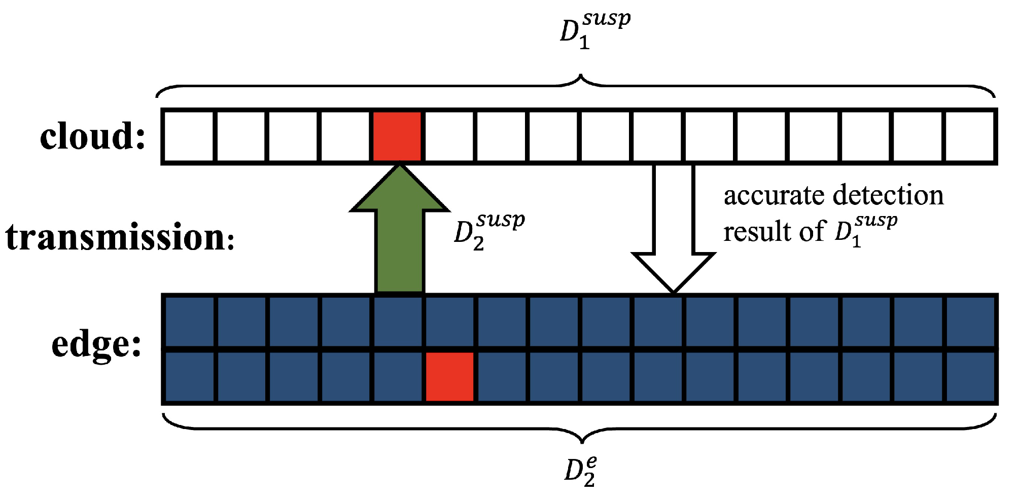
3.1. Cloud–Edge Collaboration Framework

The main principle of our algorithm is that, while the edge is capturing new hyperspectral data and performing real-time detection, some of the previously detected suspicious anomalies and their surrounding pixels are uploaded to the cloud for high-precision detection. After detecting the real anomalies, the cloud sends back the information of anomalies to the edge. The high-accuracy detection algorithm used in the cloud is the LRX algorithm, which can be replaced by other high-local-accuracy anomaly detection algorithms. These local anomaly detection algorithms can perform parallel calculations in the cloud to obtain accurate results. In particular, it is emphasized that the purpose of performing detection at the cloud is to help the edge perform more accurate background suppression and improve the accuracy of real-time detection results at the edge. In this section, we describe our new cloud–edge framework. It is the first time that this cloud–edge collaboration framework has been proposed and utilized in real-time hyperspectral detection.

We assume that the CE-RX algorithm consists of multiple rounds of cloud–edge collaboration. Figure 1 shows the data storage and transmission between the cloud and the edge when the first n pixels are captured at the edge. When performing cloud–edge interactions, the edge uploads the suspicious anomalies and their surrounding pixels (denoted as $D_1^{susp}$) to the cloud. The purpose of uploading the surrounding pixels of suspicious anomalies is to calculate the background covariance matrix in Equation (10). Here, we assume that the number of hyperspectral pixels uploaded to the cloud in each round is $k_m$. Generally, $k_m$ is much smaller than n. In the first round, there are no data available in the cloud for high-precision detection. Therefore, there are no results that can be sent back from the cloud.

During the second round of the cloud–edge collaboration (illustrated in Figure 2), the cloud performs high-precision anomaly detection on the uploaded data $D_1^{susp}$. The edge captures pixels and performs real-time anomaly detection on the newly captured pixels. After the second cloud–edge communication is performed, the cloud sends the detection results of the data $D_1^{susp}$ back to the edge. The edge uploads the data $D_2^{susp}$ to the cloud and updates the matrix in the ${\delta }^{CLP-RXD}$.

During the third round of the cloud–edge collaboration (illustrated in Figure 3), the cloud performs high-precision anomaly detection on the uploaded data $D_2^{susp}$. When the third cloud–edge communication is performed, the cloud sends the detection result of the data $D_2^{susp}$ back to the edge. The edge uploads the data $D_3^{susp}$ to the cloud and updates the matrix in the ${\delta }^{CLP-RXD}$.

3.2. Edge Updating Algorithm

We can describe the mth round ($m>1$) in general fashion as follows. When performing cloud–edge interactions, as shown in Figure 4, the cloud sends back the high-precision detection results of data $D_{m-1}^{susp}$ to the edge. The edge uploads the suspicious anomalies and their surrounding pixels $D_m^{susp}$ to the cloud and updates the matrix in ${\delta }^{CLP-RXD}$.

Once the cloud has sent the detection results back to the edge, the edge needs to update the inverse correlation matrix in the real-time detection operator for background suppression. However, recomputing a new inverse correlation matrix with the pixels stored at the edge will make the update step at the edge too cumbersome from a computational viewpoint. Frequent use of previous data also makes it impossible for edge devices to transfer pixels to other devices or servers to relieve storage pressure.

To address this issue, we proceed as follows. When the mth round of the real-time detection is accomplished, the number of all the pixels is $mn$ and the correlation inverse matrix of them is denoted as $R{\left(m\right)}^{-1}$. The cloud completes the detection and sends the information of anomalies to the edge. The edge updates the correlation inverse matrix in ${\delta }^{CLP-RXD}$.

We use $\omega$ to denote the number of anomalies detected at the cloud in the mth round and use $I_a$ to denote the index of these anomalies. If we split the $R\left(m\right)$ formula, we have

$$\begin{array}{cc}\hfill R\left(m\right)& =\frac{1}{mn}\sum _{i=1}^{mn}{x}_i{x}_i^T\hfill \\ & =\frac{1}{mn}\left(\sum _{i\in I_a}{x}_i{x}_i^T+\sum _{i\notin I_a}{x}_i{x}_i^T\right)\hfill \\ & =\frac{1}{mn}\left(\left(mn-\omega \right)R_{background}\left(m\right)+\omega R_{anomalies}\left(m\right)\right)\hfill \\ & =\frac{mn-\omega }{mn}{R}_{background}\left(m\right)+\frac{\omega }{mn}{R}_{anomalies}\left(m\right).\hfill \end{array}$$

(11)

where $R_{anomalies}\left(m\right)$ denotes the correlation matrix of the anomalies detected at the cloud and $R_{background}\left(m\right)$ denotes the correlation matrix of other background pixels. According to Equation (11), we have

$$\begin{array}{c}\hfill R_{background}\left(m\right)=\frac{mn}{mn-\omega }R\left(m\right)-\frac{w}{mn-w}{R}_{anomalies}\left(m\right).\end{array}$$

(12)

According to Woodbury’s constant equation, we have

$$\begin{array}{c}\hfill \begin{array}{c}{R}_{background}{\left(m\right)}^{-1}={\left(\frac{mn}{mn-\omega }R\left(m\right)-\frac{w}{mn-w}{R}_{anomalies}\left(m\right)\right)}^{-1}\\ =\frac{mn-w}{mn}\left(R{\left(m\right)}^{-1}+R^{*}{\left(I-R^{*}\right)}^{-1}R{\left(m\right)}^{-1}\right).\end{array}\end{array}$$

(13)

where $R^{*}=\frac{w}{mn}R{\left(m\right)}^{-1}{R}_{anomalies}\left(m\right)$. The edge updating algorithm in the mth round is shown in Algorithm 1.

Algorithm 1: Edge updating algorithm

In the first round, there are no pixels that can be processed in the cloud. As a result, the cloud cannot send its detection result to the edge for updating. Therefore, the matrix $R_{background}{\left(m\right)}^{-1}$ remains unchanged. The specific steps of the CE-RX algorithm are shown in Algorithm 2.

Algorithm 2: CE-RX algorithm

In the edge updating algorithm, the cloud only sends matrix information to the edge and the edge can update information quickly. This ensures that the detection accuracy at the edge can be improved without increasing excessive edge data updating time.

4. Time Latency Analysis of the Proposed Cloud–Edge Model

In this section, we describe the computational latency model as well as the network transmission latency model for the proposed CE-RX. After that, we analyze the whole cloud–edge collaboration system.

4.1. Computing Latency Model for the Cloud and for the Edge

We assume that the computation task can be represented by $A=\left\{L,C\right\}$, where L denotes the size of the processed data and C denotes the number of CPU cycles required to compute one-bit data in the task. These two variables can be obtained by testing in advance. In this paper, the number of CPU cycles per second is used to measure the computing power at the edge and the cloud, which are respectively denoted by $f_{comp}^{edge}$ and $f_{comp}^{cloud}$.

When the anomaly detection task is performed at the edge, the time required for the mth round of detection is

$$\begin{array}{c}\hfill \begin{array}{c}\hfill t_m^{detect,edge}=\frac{L_m^{detect}{C}_m^{detect}}{f_{comp}^{edge}}\end{array}\end{array}$$

(14)

where $L{}_m^{detect}$ denotes the hyperspectral data to be processed at the edge in the mth round when the real-time algorithm is executed. $C{}_m^{detect}$ denotes the number of CPU cycles to compute one-bit data when the detection algorithm is executed at the edge.

When the updating algorithm is executed at the edge, the update latency is

$$\begin{array}{c}\hfill \begin{array}{c}\hfill t_m^{update,edge}=\frac{L_m^{update}{C}_m^{update}}{f_{comp}^{edge}}\end{array}\end{array}$$

(15)

where $L_m^{update}$ denotes the hyperspectral data to be processed at the edge in the mth round when the update algorithm is executed. $C_m^{update}$ denotes the number of CPU cycles to compute one-bit data when the updating algorithm is executed at the edge.

Similarly, we can obtain the time spent in the mth round when the cloud performs high-accuracy detection:

$$\begin{array}{c}\hfill \begin{array}{c}\hfill t_m^{susp,cloud}=\frac{L_m^{susp}{C}_m^{susp}}{f_{comp}^{cloud}}\end{array}\end{array}$$

(16)

where $L{}_m^{susp}$ denotes the hyperspectral data to be processed at the cloud in the mth round when executing the high-precision background suppression algorithm. $C{}_m^{susp}$ denotes the number of CPU cycles for computing one-bit data in the cloud when executing the high-precision background suppression.

4.2. System Latency Model

Figure 5 shows the computational latency to be considered for the mth round of computation. To be specific, $t_m^{sups,cloud}$ denotes the time spent for computation at the cloud in round m, $t_m^{detect,edge}$ denotes the time spent for real-time detection at the edge in round m, $t_m^{cor}$ denotes the time spent for data transmission between the cloud and the edge in round m, and $t_m^{update,edge}$ denotes the latency of data updating at the edge in round m. Then, the total time $T_m$ of the cloud–edge collaborative computation at the mth round can be expressed as

$$\begin{array}{c}\hfill \begin{array}{cc}\hfill T_m& =max(t_m^{detect,edge}+t_m^{update,edge},t_m^{susp,cloud}+t_m^{cor}).\hfill \end{array}\end{array}$$

(17)

5. Experimental Results

This section is organized as follows. The hyperspectral datasets used in the experiments are first introduced in Section 5.1. Section 5.2 evaluates the detection accuracy of the software version using MATLAB of the proposed CE-RX by comparing the widely used detectors mentioned above. Section 5.3 evaluates the real-time performance of the proposed CE-RX by comparing other algorithms.

In this paper, the 3-D and 2-D receiver operating characteristic (ROC) curves [47] and the area under the curve (AUC) values are used as the evaluation criteria for experimental results. We used the AUC score of false alarm F and the probability of detection D to evaluate the performance of the anomaly detection algorithm. The closer the AUC value to 1.0, the better the detection result. Furthermore, we used the AUC score of the thresholds $\tau$ and false alarm to evaluate the performance of background suppressibility. When the value of the false alarm is 0, it means that no background pixel is mistakenly detected as an anomaly.

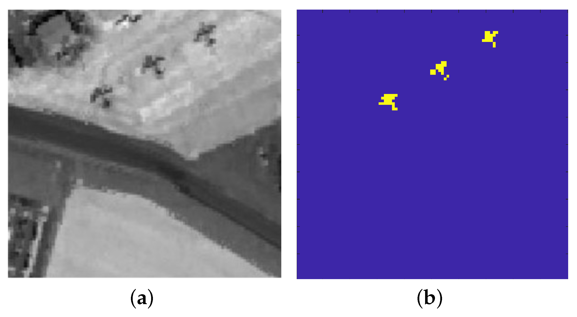
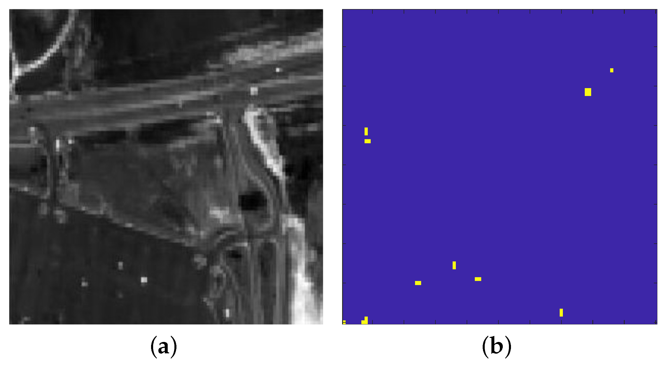
5.1. Dataset Description

To test the effectiveness and feasibility of the proposed algorithm, we selected three real datasets for comparison purposes.

Real-data1 is a hyperspectral image from San Diego Airport, collected by the airborne visible-infrared imaging spectrometer (AVIRIS). The image has 224 bands. Its spatial resolution is 3.5 m per pixel. In the pre-processing stage, we removed the water vapor bands and some contaminated bands (1–6, 33–35, 94–97, 107–113, 153–166, and 221–224). Then, 186 available bands were retained in the experiments. The experimental data came from a small area of $100\times 100$ in the upper left corner of the overall image, as shown in Figure 6a. The background part of the area consists of the apron, building roofs, and a small amount of vegetation. Figure 6b shows the ground-truth map of the real anomalies. The anomalies are three aircraft on the tarmac and contain 57 pixels.

Real-data2 is a Salinas hyperspectral image collected by the airborne visible-infrared imaging spectrometer (AVIRIS). The image has 224 bands. Its spatial resolution is 3.7 m per pixel. In the pre-processing stage, we removed some contaminated bands (108–112, 154–167, 205). Then, 204 available bands of the data were retained in the experiments. The experimental data came from a small area of $100\times 100$ in the bottom left corner of the overall image, as shown in Figure 7a. Figure 7b shows the ground-truth map of the real anomalies.

Real-data3 is an urban hyperspectral image acquired over Texas, USA, by the hyperspectral data collection experiment (HYDICE) instrument. The image has 210 bands. Its spatial resolution is 1 m per pixel. In the pre-processing stage, we removed the water vapor bands and some contaminated bands (1–4, 76, 87, 101–111, 136–153, 198–210). Then, 162 available bands of the data were retained in the experiments. The experimental data came from a small area of $80\times 100$ in the upper right corner of the overall image, as shown in Figure 8a. The background part of the area consists of roads, grass, and trees. Figure 8b shows the ground-truth map of the real anomalies. The anomalies are cars in the region and contain 21 pixels.

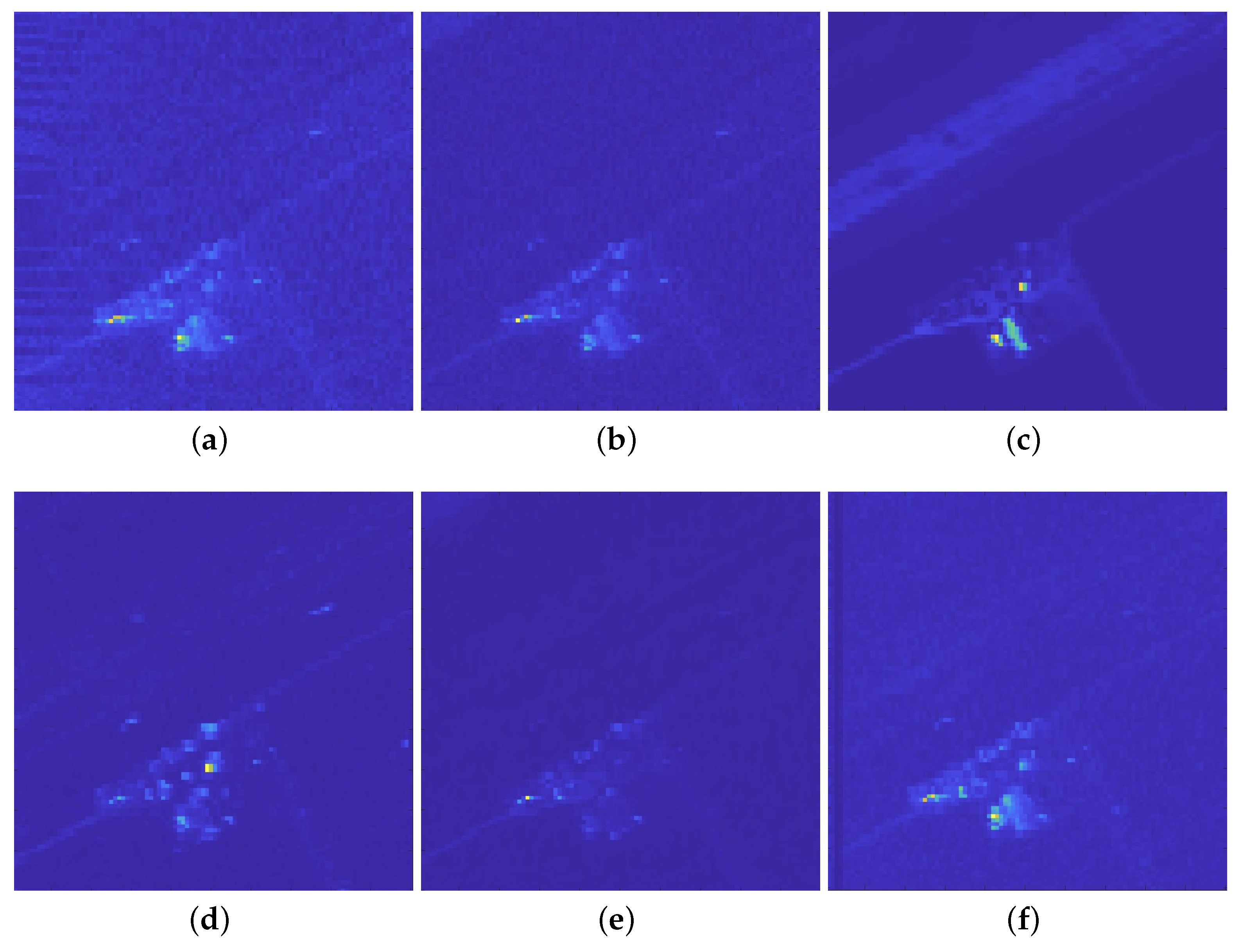
5.2. Detection Performance

In order to evaluate detection accuracy, we compared the proposed CE-RX algorithm with the following anomaly detection algorithms: CLP-RX algorithm, LRASR algorithm [48], RGAE algorithm [49], LSUNRSOR algorithm [50], and FEBP algorithm [51]. To test the real-time detection accuracy, we executed these algorithms following the scenario of capturing and detecting data in real time. The CE-RX algorithm performs one cloud–edge interaction for every 500 captured pixels at the edge. The simulation environment in the experiment was a 64-bit system. The CPU was an Intel(R) Core(TM) i5-7300HQ operating at 2.50 GHz. The system memory was 8 G. The software used for implementation was MATLAB R2018b.

For the real-data1, the anomalies were three aircrafts. Figure 9 shows the results of the comparison experiments. Figure 10 plots the ROC curve generated from the results in Figure 9.

Table 2. AUC for the detection algorithms in Figure 9.

Detector	${\mathit{AUC}}_{\left(\mathit{D},\mathit{F}\right)}$	${\mathit{AUC}}_{\left(\mathit{F},\mathit{\tau }\right)}$
CLP-RX (real-time)	0.9225	0.0821
LRASR (non-real-time)	0.9948	0.0786
RGAR (non-real-time)	0.9887	0.0365
LSUNRSOR (non-real-time)	0.9579	0.0737
FEBP (non-real-time)	0.9791	0.0050
CE-RX (real-time)	0.9933	0.0783

tabulates the AUC values of $\left(D,F\right)$ and $\left(F,\tau \right)$ for quantitative studies and analysis, the best detection results are highlighted in bold. It is noticeable that the CE-RX algorithm has a good detection result. The detection performance of the CE-RX algorithm is better than all other detection algorithms except slightly lower than the LRASR algorithm. On the contrary, The CLP-RX algorithm exhibits relatively poor accuracy due to the limitations of the real-time algorithm. It can be observed that the CE-RX method can effectively identify anomalies with 0.9974 as the AUC score of $\left(D,F\right)$. We observed that the AUC values of the CE-RX algorithm are 0.0708 higher than the AUC values of the CLP-RX algorithm. This observation proves that the cloud–edge collaborative approach can greatly improve the detection accuracy of the algorithm at the edge.

In each round of the cloud–edge interaction in the CE-RX algorithm, the lower the number of pixels uploaded from the edge to the cloud, the larger the number of cloud–edge interactions. To verify the effect of the number of cloud–edge interactions on the considered algorithm, we performed four sets of experiments denoted by experiment1, experiment2, experiment3, and experiment4. In experiment1, the algorithm performs one cloud–edge interaction for every 2000 pixels captured at the edge. In experiment2, the algorithm performs one cloud–edge interaction for every 1000 pixels captured at the edge. In experiment3, the algorithm performs one cloud–edge interaction for every 500 captured pixels at the edge. In experiment4, the algorithm does not perform cloud–edge interactions. We compare the detection results of the CE-RX algorithm in three sets of experiments. The AUC is shown in

Table 3. AUC for the four sets of experiments on the real-data1.

	Experiment1	Experiment2	Experiment3	Experiment4
AUC	0.9591	0.9757	0.9933	0.9225

. We can see that more cloud–edge interactions lead to better results.

Figure 11 shows the detection results of different algorithms on the real-data2. Figure 12 shows the corresponding ROC curves.

Table 4. AUC for the detection algorithms in Figure 11.

Detector	${\mathit{AUC}}_{\left(\mathit{D},\mathit{F}\right)}$	${\mathit{AUC}}_{\left(\mathit{F},\mathit{\tau }\right)}$
CLP-RX (real-time)	0.9070	0.0446
LRASR (non-real-time)	0.9826	0.0246
RGAR (non-real-time)	0.9767	0.0115
LSUNRSOR (non-real-time)	0.9753	0.0124
FEBP (non-real-time)	0.9690	0.0062
CE-RX (real-time)	0.9842	0.0348

shows the AUC values of all detection algorithms and the best detection results are highlighted in bold. The proposed algorithm is the most effective in detecting and has the highest AUC value (0.9842). Based on real-data2, we also perform four sets of experiments again using the CE-RX algorithm. The experiments are denoted by experiment1, experiment2, experiment3, and experiment4. In experiment1, the algorithm performs one cloud–edge interaction for every 2000 pixels captured. In experiment2, the algorithm performs one cloud–edge interaction for every 1000 pixels captured. In experiment3, one cloud–edge interaction is performed for every 500 pixels captured at the edge. In experiment4, the algorithm does not perform cloud–edge interaction.

Table 5. AUC for the four sets of experiments on the real-data2.

	Experiment1	Experiment2	Experiment3	Experiment4
AUC	0.9206	0.9538	0.9842	0.9070

shows the AUC values of the four sets of experiments. We can still see that more cloud–edge interactions lead to better results.

The anomalies of real-data3 are multiple cars. Compared to the anomalies of other datasets, the anomalies of real-data3 take up a relatively smaller proportion of the whole picture. The CLP-RX real-time algorithm not only has difficulty in detecting larger objects but also has low detection results for smaller objects. We can observe that the CE-RX algorithm has a better detection result than other detection algorithms. The AUC values of all algorithms are given in

Table 6. AUC for the detection algorithms in Figure 13.

Detector	${\mathit{AUC}}_{\left(\mathit{D},\mathit{F}\right)}$	${\mathit{AUC}}_{\left(\mathit{F},\mathit{\tau }\right)}$
CLP-RX (real-time)	0.8567	0.0540
LRASR (non-real-time)	0.9438	0.0570
RGAR (non-real-time)	0.9311	0.0516
LSUNRSOR (non-real-time)	0.9553	0.0544
FEBP (non-real-time)	0.9590	0.0429
CE-RX (real-time)	0.9642	0.0418

and the best detection results are highlighted in bold. The results of detection are shown in Figure 13, and the ROC curves are given in Figure 14. We can see that the AUC value of the CE-RX algorithm is 0.9642, which is higher than the AUC value of the CLP-RX algorithm. These results prove that the CE-RX algorithm exhibits higher detection accuracy when hyperspectral images contain anomalies with small-scale differences.

Once again, we perform four sets of experiments as with the previous two datasets. The experiments are denoted by experiment1, experiment2, experiment, and experiment4.

Table 7. AUC for the four sets of experiments on the real-data3.

	Experiment1	Experiment2	Experiment3	Experiment4
AUC	0.9362	0.9595	0.9642	0.8567

shows the AUC values. We can see that the higher the frequency of cloud–edge collaboration, the more accurate the CE-RX algorithm will be in detecting anomalies in the real-data3.

5.3. Real-time Performance Analysis of Proposed Algorithms

To evaluate the computing latency of our proposed algorithm, we conducted extensive experiments on a Jetson AGX Orin development board and a cloud server. The Jetson AGX Orin development board is equipped with a 12-core Cortex-A78 arm processor, a 2048-core GPU with 64 Tensor Cores, and 32GB RAM. The cloud server is composed of three hosts equipped with 18 core i9-10980K CPU, 128GB RAM, and 1T disk storage.

Table 8. Computational latency of the CE-RX algorithm.

Hyperspectral Data	${\mathit{t}}_{\mathit{total}}^{\mathit{cor}}$	${\mathit{t}}_{\mathit{total}}^{\mathit{detect},\mathit{edge}}$	${\mathit{t}}_{\mathit{total}}^{\mathit{susp},\mathit{cloud}}$	${\mathit{t}}_{\mathit{total}}^{\mathit{update},\mathit{edge}}$	${\mathit{T}}_{\mathit{total}}$
real-data1	54 ms	87 ms	21 ms	4 ms	91 ms
real-data2	45 ms	85 ms	20 ms	5 ms	90 ms
real-data3	42 ms	79 ms	20 ms	5 ms	84 ms

shows the computational latency of the CE-RX algorithm on the three hyperspectral datasets. In the experiment, we perform ten cloud–edge interactions. We can see that the latency for the edge to perform real-time detection is longer than the latency for the edge to upload the data to the cloud and perform high-accuracy detection, i.e., $t_m^{detect,edge}>t_m^{cor}+t^{susp,cloud}$. Therefore, the total latency of the CE-RX algorithm $T_{total}$ is the computational latency at the edge plus the latency for the edge to receive the results from the cloud and perform the update algorithm:

$$\begin{array}{c}\hfill \begin{array}{c}\hfill T_{total}=t_{total}^{detect,edge}+t_{total}^{update,edge}\end{array}.\end{array}$$

(18)

As shown in Table 8, we know that $t_{total}^{detect,edge}>>t_{total}^{update,edge}$, data updates at the edge do not affect the real-time performance of the CE-RX algorithm. From

Table 9. Computational latency of all algorithms.

Hyperspectral Data	Real-Data1	Real-Data2	Real-Data3
CLP-RX (real-time)	0.087 s	0.085 s	0.079 s
LRASR (non-real-time)	202 s	131 s	182 s
RGAR (non-real-time)	436 s	421 s	401 s
LSUNRSOR (non-real-time)	221 s	232 s	212 s
FEBP (non-real-time)	11.2 s	12.9 s	10.1 s
CE-RX (real-time)	0.091 s	0.09 s	0.084 s

, we can see that both the CLP-RX and CE-RX algorithms have excellent real-time performance. The computation latency of the CLP-RX algorithm and the CE-RX algorithm are much smaller than the computation latency of other algorithms. Although the computation latency of the CE-RX algorithm is longer than that of the CLP algorithm, the extra time is the latency of performing the data update at the edge. Therefore, the CE-RX algorithm significantly improves the accuracy of the detection results at the cost of slightly increasing the overall computational latency.

To verify the scalability of the CE-RX algorithm, we join the real-data1 to generate data of 1 GB, 2 GB, 4 GB, and 8 GB, respectively, and performed experiments on the condition that the CE-RX algorithm performs one cloud–edge interaction for every 500 captured pixels at the edge. The results are shown in

Table 10. Latency corresponding to different data sizes.

Data Size	Latency	Latency Ratio
1 GB	34.52 s	1
2 GB	70.11 s	2.03
4 GB	142.64 s	4.13
8 GB	282.81 s	8.19

. It is obvious that the latency increases with the growth of data size. The latency of updating the algorithm does not increase linearly as the data volume grows, which results in nonlinear growth of the total running time. In general, the experiments indicate that the CE-RX algorithm is scalable for larger data.

6. Discussion

In the experiment, the proposed algorithm was compared with the other five algorithms. Experimental results on three real datasets illustrate the advantage of the proposed CE-RX method. While ensuring real-time performance, the CE-RX algorithm has high detection accuracy. We again set different numbers of cloud–edge interactions to verify the effectiveness of detection. We can see that the higher the number of edge interactions, the higher the accuracy of the CE-RX algorithm will be. If there is no cloud–edge interaction performed, the CE-RX has the same accuracy as the CLP algorithm.

When performing the cloud–edge interaction, the cloud only needs to send back the information about the anomalies detected in this round. This makes the latency of network transmission negligible. In addition, the update algorithm at the edge makes it so that the edge does not need to recalculate the correlation matrix of all background pixels after receiving the information of the anomalies. This makes the latency of data updating much lower. As can be seen from Table 8, the latency for the edge to update is only $6\%$ of $T_{total}$. Since the computation latency of the update algorithm is determined by the participating matrices $R_{anomalies}\left(m\right)$ and $R\left(m\right)$, the total computation latency does not change with the increase of captured data. This means that no matter how much data are captured at the edge, the update time is constant for each cloud–edge interaction. Therefore, this algorithm is scalable for larger data. The push-scan spectrometer can capture tens of thousands of pixels per second. One second to perform a cloud–edge interaction will only result in an additional 0.5 ms of edge update. This does not affect the overall real-time performance of the algorithm.

7. Conclusions

In this paper, we propose a hyperspectral anomaly detection algorithm based on the cloud–edge collaboration called CE-RX. While pixels are captured at the edge, this algorithm performs real-time anomaly detection on them to obtain a fast result. Then, the suspicious anomalies are uploaded to the cloud in the edge so that the cloud can use its vast computing resources to perform highly accurate algorithms on the uploaded data, find the real anomalies, and send them back to the edge for data updates, so as to improve the accuracy of the next round of real-time anomaly detection. This represents a completely innovative approach to anomaly detection in hyperspectral images. Our experimental results demonstrate that the newly proposed CE-RX algorithm exhibits higher accuracy compared with existing real-time detection algorithms while ensuring real-time performance.

References

1. Zhang, B.; Sun, X.; Gao, L.; Yang, L. Endmember Extraction of Hyperspectral Remote Sensing Images Based on the Ant Colony Optimization (ACO) Algorithm. IEEE Trans. Geosci. Remote Sens. 2011, 49, 2635–2646. [Google Scholar] [CrossRef]
2. Zhang, B.; Liu, Y.; Zhang, W.; Gao, L.; Li, J.; Wang, J.; Li, X. Analysis of the proportion of surface reflected radiance in mid-infrared absorption bands. IEEE J. Sel. Top. Appl. Earth Obs. Remote Sens. 2013, 7, 2639–2646. [Google Scholar] [CrossRef]
3. Gao, L.; Du, Q.; Zhang, B.; Yang, W.; Wu, Y. A Comparative Study on Linear Regression-Based Noise Estimation for Hyperspectral Imagery. IEEE J. Sel. Top. Appl. Earth Obs. Remote Sens. 2013, 6, 488–498. [Google Scholar] [CrossRef]
4. Li, S.; Song, W.; Fang, L.; Chen, Y.; Ghamisi, P.; Benediktsson, J.A. Deep learning for hyperspectral image classification: An overview. IEEE Trans. Geosci. Remote Sens. 2019, 57, 6690–6709. [Google Scholar] [CrossRef]
5. Wang, Y.; Chen, X.; Wang, F.; Song, M.; Yu, C. Meta-learning based hyperspectral target detection using Siamese network. IEEE Trans. Geosci. Remote Sens. 2022, 60, 5527913. [Google Scholar] [CrossRef]
6. Song, M.; Liu, S.; Xu, D.; Yu, H. Multiobjective optimization-based hyperspectral band selection for target detection. IEEE Trans. Geosci. Remote Sens. 2022, 60, 5529022. [Google Scholar] [CrossRef]
7. Chen, J.; Chang, C.I. Background-Annihilated Target-Constrained Interference-Minimized Filter (TCIMF) for Hyperspectral Target Detection. IEEE Trans. Geosci. Remote Sens. 2022, 60, 5540224. [Google Scholar] [CrossRef]
8. Chen, Z.; Lu, Z.; Gao, H.; Zhang, Y.; Zhao, J.; Hong, D.; Zhang, B. Global to local: A hierarchical detection algorithm for hyperspectral image target detection. IEEE Trans. Geosci. Remote Sens. 2022, 60, 5544915. [Google Scholar] [CrossRef]
9. Gao, H.; Zhang, Y.; Chen, Z.; Xu, S.; Hong, D.; Zhang, B. A Multidepth and Multibranch Network for Hyperspectral Target Detection Based on Band Selection. IEEE Trans. Geosci. Remote Sens. 2023, 61, 5506818. [Google Scholar] [CrossRef]
10. Gao, H.; Zhang, Y.; Chen, Z.; Xu, F.; Hong, D.; Zhang, B. Hyperspectral Target Detection via Spectral Aggregation and Separation Network with Target Band Random Mask. IEEE Trans. Geosci. Remote Sens. 2023, 61, 5515516. [Google Scholar] [CrossRef]
11. Jia, S.; Jiang, S.; Lin, Z.; Li, N.; Xu, M.; Yu, S. A survey: Deep learning for hyperspectral image classification with few labeled samples. Neurocomputing 2021, 448, 179–204. [Google Scholar] [CrossRef]
12. Xie, H.; Chen, Y.; Ghamisi, P. Remote sensing image scene classification via label augmentation and intra-class constraint. Remote Sens. 2021, 13, 2566. [Google Scholar] [CrossRef]
13. Liu, S.; Cao, Y.; Wang, Y.; Peng, J.; Mathiopoulos, P.T.; Li, Y. DFL-LC: Deep feature learning with label consistencies for hyperspectral image classification. IEEE J. Sel. Top. Appl. Earth Obs. Remote Sens. 2021, 14, 3669–3681. [Google Scholar] [CrossRef]
14. Li, W.; Du, Q. Collaborative representation for hyperspectral anomaly detection. IEEE Trans. Geosci. Remote Sens. 2014, 53, 1463–1474. [Google Scholar] [CrossRef]
15. Xie, W.; Zhang, X.; Li, Y.; Lei, J.; Li, J.; Du, Q. Weakly supervised low-rank representation for hyperspectral anomaly detection. IEEE Trans. Cybern. 2021, 51, 3889–3900. [Google Scholar] [CrossRef] [PubMed]
16. Jiang, T.; Xie, W.; Li, Y.; Lei, J.; Du, Q. Weakly supervised discriminative learning with spectral constrained generative adversarial network for hyperspectral anomaly detection. IEEE Trans. Neural Networks Learn. Syst. 2021, 33, 6504–6517. [Google Scholar] [CrossRef]
17. Reed, I.S.; Yu, X. Adaptive multiple-band CFAR detection of an optical pattern with unknown spectral distribution. IEEE Trans. Acoust. Speech Signal Process. 1990, 38, 1760–1770. [Google Scholar] [CrossRef]
18. Yu, X.; Reed, I.S.; Stocker, A.D. Comparative performance analysis of adaptive multispectral detectors. IEEE Trans. Signal Process. 1993, 41, 2639–2656. [Google Scholar] [CrossRef]
19. Li, C.; Zhang, B.; Hong, D.; Yao, J.; Chanussot, J. LRR-Net: An Interpretable Deep Unfolding Network for Hyperspectral Anomaly Detection. IEEE Trans. Geosci. Remote Sens. 2023, 61, 5513412. [Google Scholar] [CrossRef]
20. Gao, L.; Sun, X.; Sun, X.; Zhuang, L.; Du, Q.; Zhang, B. Hyperspectral anomaly detection based on chessboard topology. IEEE Trans. Geosci. Remote Sens. 2023, 61, 5505016. [Google Scholar] [CrossRef]
21. Wang, M.; Hong, D.; Zhang, B.; Ren, L.; Yao, J.; Chanussot, J. Learning double subspace representation for joint hyperspectral anomaly detection and noise removal. IEEE Trans. Geosci. Remote Sens. 2023, 61, 5507517. [Google Scholar] [CrossRef]
22. Horstrand, P.; Díaz, M.; Guerra, R.; López, S.; López, J.F. A novel hyperspectral anomaly detection algorithm for real-time applications with push-broom sensors. IEEE J. Sel. Top. Appl. Earth Obs. Remote Sens. 2019, 12, 4787–4797. [Google Scholar] [CrossRef]
23. Báscones, D.; González, C.; Mozos, D. An FPGA accelerator for real-time lossy compression of hyperspectral images. Remote Sens. 2020, 12, 2563. [Google Scholar] [CrossRef]
24. Li, C.; Gao, L.; Plaza, A.; Zhang, B. FPGA implementation of a maximum simplex volume algorithm for endmember extraction from remotely sensed hyperspectral images. J. Real-Time Image Process. 2019, 16, 1681–1694. [Google Scholar] [CrossRef]
25. Du, Q.; Ren, H. Real-time constrained linear discriminant analysis to target detection and classification in hyperspectral imagery. Pattern Recognit. 2003, 36, 1–12. [Google Scholar] [CrossRef]
26. Chang, C.I.; Ren, H.; Chiang, S.S. Real-time processing algorithms for target detection and classification in hyperspectral imagery. IEEE Trans. Geosci. Remote Sens. 2001, 39, 760–768. [Google Scholar] [CrossRef]
27. Zhao, C.; Wang, Y.; Qi, B.; Wang, J. Global and local real-time anomaly detectors for hyperspectral remote sensing imagery. Remote Sens. 2015, 7, 3966–3985. [Google Scholar] [CrossRef]
28. Chen, S.Y.; Wang, Y.; Wu, C.C.; Liu, C.; Chang, C.I. Real-time causal processing of anomaly detection for hyperspectral imagery. IEEE Trans. Aerosp. Electron. Syst. 2014, 50, 1511–1534. [Google Scholar] [CrossRef]
29. Wang, Y.; Chen, S.Y.; Wu, C.C.; Liu, C.; Chang, C.I. Real-time causal processing of anomaly detection. In Proceedings of the High-Performance Computing in Remote Sensing II. SPIE, Edinburgh, UK, 26–27 September 2012; Volume 8539, pp. 50–57. [Google Scholar]
30. Zhao, C.; Li, C.; Yao, X.; Li, W. Real-time kernel collaborative representation-based anomaly detection for hyperspectral imagery. Infrared Phys. Technol. 2020, 107, 103325. [Google Scholar] [CrossRef]
31. Ndikumana, A.; Tran, N.H.; Ho, T.M.; Han, Z.; Saad, W.; Niyato, D.; Hong, C.S. Joint communication, computation, caching, and control in big data multi-access edge computing. IEEE Trans. Mob. Comput. 2019, 19, 1359–1374. [Google Scholar] [CrossRef]
32. Pan, J.; McElhannon, J. Future edge cloud and edge computing for internet of things applications. IEEE Internet Things J. 2017, 5, 439–449. [Google Scholar] [CrossRef]
33. Premsankar, G.; Di Francesco, M.; Taleb, T. Edge computing for the Internet of Things: A case study. IEEE Internet Things J. 2018, 5, 1275–1284. [Google Scholar] [CrossRef]
34. Zhang, Y.; Lan, X.; Ren, J.; Cai, L. Efficient computing resource sharing for mobile edge-cloud computing networks. IEEE/ACM Trans. Netw. 2020, 28, 1227–1240. [Google Scholar] [CrossRef]
35. Xu, X.; Liu, Q.; Luo, Y.; Peng, K.; Zhang, X.; Meng, S.; Qi, L. A computation offloading method over big data for IoT-enabled cloud-edge computing. Future Gener. Comput. Syst. 2019, 95, 522–533. [Google Scholar] [CrossRef]
36. Xu, X.; Gu, R.; Dai, F.; Qi, L.; Wan, S. Multi-objective computation offloading for internet of vehicles in cloud-edge computing. Wirel. Netw. 2020, 26, 1611–1629. [Google Scholar] [CrossRef]
37. Ren, J.; Yu, G.; He, Y.; Li, G.Y. Collaborative cloud and edge computing for latency minimization. IEEE Trans. Veh. Technol. 2019, 68, 5031–5044. [Google Scholar] [CrossRef]
38. Jia, M.; Cao, J.; Yang, L. Heuristic offloading of concurrent tasks for computation-intensive applications in mobile cloud computing. In Proceedings of the 2014 IEEE Conference on Computer Communications Workshops (INFOCOM WKSHPS), Toronto, ON, Canada, 27 April–2 May 2014; pp. 352–357. [Google Scholar]
39. Zhang, X.; Hu, M.; Xia, J.; Wei, T.; Chen, M.; Hu, S. Efficient federated learning for cloud-based AIoT applications. IEEE Trans. Comput.-Aided Des. Integr. Circuits Syst. 2020, 40, 2211–2223. [Google Scholar] [CrossRef]
40. Gu, H.; Ge, Z.; Cao, E.; Chen, M.; Wei, T.; Fu, X.; Hu, S. A collaborative and sustainable edge-cloud architecture for object tracking with convolutional siamese networks. IEEE Trans. Sustain. Comput. 2019, 6, 144–154. [Google Scholar] [CrossRef]
41. Gamez, G.; Frey, D.; Michler, J. Push-broom hyperspectral imaging for elemental mapping with glow discharge optical emission spectrometry. J. Anal. At. Spectrom. 2012, 27, 50–55. [Google Scholar] [CrossRef]
42. Zhang, L.; Peng, B.; Zhang, F.; Wang, L.; Zhang, H.; Zhang, P.; Tong, Q. Fast real-time causal linewise progressive hyperspectral anomaly detection via cholesky decomposition. IEEE J. Sel. Top. Appl. Earth Obs. Remote Sens. 2017, 10, 4614–4629. [Google Scholar] [CrossRef]
43. Molero, J.M.; Garzon, E.M.; Garcia, I.; Plaza, A. Analysis and optimizations of global and local versions of the RX algorithm for anomaly detection in hyperspectral data. IEEE J. Sel. Top. Appl. Earth Obs. Remote Sens. 2013, 6, 801–814. [Google Scholar] [CrossRef]
44. Chang, C.; Chiang, S. Anomaly detection and classification for hyperspectral imagery. IEEE Trans. Geosci. Remote Sens. 2002, 40, 1314–1325. [Google Scholar] [CrossRef]
45. Chen, X.; Gu, C.; Zhang, Y.; Mittra, R. Analysis of partial geometry modification problems using the partitioned-inverse formula and Sherman–Morrison–Woodbury formula-based method. IEEE Trans. Antennas Propag. 2018, 66, 5425–5431. [Google Scholar] [CrossRef]
46. Xu, X. Generalization of the Sherman–Morrison–Woodbury formula involving the Schur complement. Appl. Math. Comput. 2017, 309, 183–191. [Google Scholar] [CrossRef]
47. Chang, C.I. An effective evaluation tool for hyperspectral target detection: 3D receiver operating characteristic curve analysis. IEEE Trans. Geosci. Remote Sens. 2020, 59, 5131–5153. [Google Scholar] [CrossRef]
48. Xu, Y.; Wu, Z.; Li, J.; Plaza, A.; Wei, Z. Anomaly detection in hyperspectral images based on low-rank and sparse representation. IEEE Trans. Geosci. Remote Sens. 2015, 54, 1990–2000. [Google Scholar] [CrossRef]
49. Fan, G.; Ma, Y.; Huang, J.; Mei, X.; Ma, J. Robust graph autoencoder for hyperspectral anomaly detection. In Proceedings of the ICASSP 2021-2021 IEEE International Conference on Acoustics, Speech and Signal Processing (ICASSP), Toronto, ON, Canada, 6–11 June 2021; pp. 1830–1834. [Google Scholar]
50. Tan, K.; Hou, Z.; Wu, F.; Du, Q.; Chen, Y. Anomaly detection for hyperspectral imagery based on the regularized subspace method and collaborative representation. Remote Sens. 2019, 11, 1318. [Google Scholar] [CrossRef]
51. Ma, Y.; Fan, G.; Jin, Q.; Huang, J.; Mei, X.; Ma, J. Hyperspectral anomaly detection via integration of feature extraction and background purification. IEEE Geosci. Remote Sens. Lett. 2020, 18, 1436–1440. [Google Scholar] [CrossRef]
Figure 1. Data storage and transmission for round 1 of the proposed cloud–edge collaboration.
Remotesensing 15 04242 g001
Figure 2. Data storage and transmission for round 2 of the proposed cloud–edge collaboration.
Remotesensing 15 04242 g002
Figure 3. Data storage and transmission for round 3 of the proposed cloud–edge collaboration.
Remotesensing 15 04242 g003
Figure 4. Data storage and transmission for round m of the proposed cloud–edge collaboration.
Remotesensing 15 04242 g004
Figure 5. Overview of the system latency model.
Remotesensing 15 04242 g005
Figure 6. Real-data1. (a) Original image. (b) Ground-truth map.
Remotesensing 15 04242 g006
Figure 7. Real-data2. (a) Original image; (b) Ground-truth map.
Remotesensing 15 04242 g007
Figure 8. Real-data3. (a) Original image. (b) Ground-truth map.
Remotesensing 15 04242 g008
Figure 9. Detection performance of different algorithms for real-data1. (a) CLP-RX Algorithm; (b) LRASR Algorithm; (c) RGAE Algorithm; (d) LSUNRSOR Algorithm; (e) FEBP Algorithm; (f) CE-RX Algorithm.
Remotesensing 15 04242 g009
Figure 10. ROC curves obtained by different methods for real-data1. (a) 3D ROC curves; (b) ROC curves of F , τ .
Remotesensing 15 04242 g010
Figure 11. Detection performance of different algorithms for real-data2. (a) CLP-RX Algorithm; (b) LRASR Algorithm; (c) RGAE Algorithm; (d) LSUNRSOR Algorithm; (e) FEBP Algorithm; (f) CE-RX Algorithm.
Remotesensing 15 04242 g011
Figure 12. ROC curves obtained by different methods for real-data2. (a) 3D ROC curves; (b) ROC curves of F , τ .
Remotesensing 15 04242 g012
Figure 13. Detection performance of different algorithms for real-data3. (a) CLP-RX Algorithm; (b) LRASR Algorithm; (c) RGAE Algorithm; (d) LSUNRSOR Algorithm; (e) FEBP Algorithm; (f) CE-RX Algorithm.
Remotesensing 15 04242 g013
Figure 14. ROC curves obtained by different methods for real-data3. (a) 3D ROC curves; (b) ROC curves of F , τ .
Remotesensing 15 04242 g014