Article

RemainNet: Explore Road Extraction from Remote Sensing Image Using Mask Image Modeling

1
College of Electronic Science and Technology, National University of Defense Technology, Changsha 410073, China
2
Key Laboratory of Natural Resources Monitoring and Supervision in Southern Hilly Region, Ministry of Natural Resources, Changsha 410073, China
*
Author to whom correspondence should be addressed.
Remote Sens. 2023, 15(17), 4215; https://doi.org/10.3390/rs15174215
Submission received: 26 June 2023 / Revised: 24 August 2023 / Accepted: 25 August 2023 / Published: 28 August 2023

Abstract

:
Road extraction from a remote sensing image is a research hotspot due to its broad range of applications. Despite recent advancements, achieving precise road extraction remains challenging. Since a road is thin and long, roadside objects and shadows cause occlusions, thus influencing the distinguishment of the road. Masked image modeling reconstructs masked areas from unmasked areas, which is similar to the process of inferring occluded roads from nonoccluded areas. Therefore, we believe that mask image modeling is beneficial for indicating occluded areas from other areas, thus alleviating the occlusion issue in remote sensing image road extraction. In this paper, we propose a remote sensing image road extraction network named RemainNet, which is based on mask image modeling. RemainNet consists of a backbone, image prediction module, and semantic prediction module. An image prediction module reconstructs a masked area RGB value from unmasked areas. Apart from reconstructing original remote sensing images, a semantic prediction module of RemainNet also extracts roads from masked images. Extensive experiments are carried out on the Massachusetts Roads dataset and DeepGlobe Road Extraction dataset; the proposed RemainNet improves 0.82–1.70% IoU compared with other state-of-the-art road extraction methods.

1. Introduction

With the development of remote sensing (RS) technology, a large number of high-resolution RS images are available [1]. Thus, RS image interpretation has been widely applied in many fields, such as urban management [2], map updating [3], and traffic planning [4].
Conventional road extraction methods usually use manually design features (such as geometric features and texture features) [5] and adopt traditional machine learning techniques (such as support vector machines and Markov random field) [5,6]. However, these conventional methods tend to be more inaccurate than later data-driven methods when dealing with big data [5]. With the development of deep learning, road extraction methods are mainly based on deep neural networks, especially convolutional neural network and transformer. Since deep leaning has shown great success, and RS image road extraction can be seen as a binary semantic segmentation task, deep learning semantic segmentation–based methods are mainstream of road extraction [7].
Although previous works have had improvements, road extraction from an RS image is still challenging [8]. Since the shape of a road is thin and long, roadside objects (such as trees and buildings) and shadows cause occlusions, as shown in Figure 1. Some works notice the occlusion problem and try to solve the issue by attention mechanism [9,10,11], centerline or edge detection [12,13,14], or context information [15,16,17]. These methods either improve the network feature extraction ability or utilize extra information, rather than enhancing the model’s area interactions (i.e., learn the interactions between different patches for reconstructing masked patches).
In recent years, masked image modeling (MIM) has shown great success in self-supervised learning. MIM improves area interactions [18] by reconstructing masked areas from unmasked areas, which is similar to the process of inferring occluded road areas from RS images in a road extraction task. Since the road is linear, the road predictions on occluded areas can be inferred by other nonoccluded areas. The introduction of MIM may improve the network contextual inference ability, thus improving the road prediction performance of occluded areas.
In this paper, we explore the practicability of road extraction from an RS image using masked image modeling (RemainNet). To the best of our knowledge, this is the first work that introduces MIM into an RS image road extraction task. Since Swin Transformer [19] is a hierarchical vision transformer that achieves an impressive performance, we adopt Swin Transformer as a backbone. In order to adopt MIM into the proposed model, we design an image prediction module (IPM) and semantic prediction module (SPM). IPM reconstructs an image from shallow features. SPM is employed to reconstruct semantic information and to conduct road predictions from masked RS images.
To summarize, the main contributions of this work are as follows:
  • We introduce MIM to enforce interactions of occluded areas with other areas, thus improving the network inference ability on occluded areas. To the best of our knowledge, it is the first RS image road extraction work based on MIM.
  • The proposed RemainNet adopts IPM and SPM for reconstruction. IPM reconstructs original images at the RGB level from low-level features. SPM reconstructs semantic labels at the semantic level from low-level and high-level features.
  • We verify the effectiveness of the proposed RemainNet on a Massachusetts Roads dataset and DeepGlobe Road Extraction dataset, and the results indicate that RemainNet outperforms other state-of-the-art methods.
The remainder of this paper is organized as follows: Section 2 introduces related work of semantic segmentation, road extraction, and masked image modeling. The proposed RemainNet is illustrated in Section 3. Section 4 conducts an experiment and displays the results. In Section 5, we provide a comprehensive discussion. Section 6 draws the conclusions of the paper.

2. Related Works

2.1. Semantic Segmentation

Semantic segmentation is a basic task in computer vision, which refers to assigning a semantic label to each pixel of an image. Before the popularity of deep learning, traditional semantic segmentation methods exploited contextual information from an image based on manually designed features [20] (such as SIFT and HOG) and traditional machine learning methods [21] (such as random forest and conditional random field). Because deep-learning-based methods achieve remarkable performance, deep-learning-based methods have become the mainstream of semantic segmentation [22].
Typical semantic segmentation models [22] are mainly FCN [23], U-Net [24], SegNet [25], and DeepLab [26,27]. FCN [23] is a revolutionary model, [28] which replaces traditional fully connected layers with convolutional layers and a proposed skip architecture. U-Net [24] is a U-shaped model with convolutional layers, deconvolutional layers, and skip connection. U-Net can obtain precise predictions with very few training images because of its elegant architecture. SegNet [25] is based on an encoder–decoder structure, and its pooling operation in an encoder retains max value places to upsample more precisely in a decoder. DeepLab v3+ [27] adopts atrous spatial pyramid pooling (ASPP), depthwise separable convolution, and an encoder–decoder structure. It outperforms previous models in the PASCAL VOC 2012 dataset.
Since the vision transformer [29] has gained great achievement in computer vision, many recent semantic segmentation methods adopt a transformer [30]. The model structure with a transformer [31] can be divided into pure transformer [29,32] and transformer with convolution [33,34]. The former utilizes the global information extraction ability of the transformer; the latter adopts a convolution neural network to improve the local feature extraction ability. Zheng et al. [32] proposed a pure transformer semantic segmentation model, which avoids gradually reducing spatial resolution like on previous methods. Robin et al. [35] proposed a fully transformer-based encoder–decoder architecture network for semantic segmentation. SegFormer [36] is a simple but efficient network, which adopts a transformer as an encoder and adopts a multilayer perceptron as a decoder. TrSeg [37] contains a CNN backbone, a multiscale pooling module, and a transformer decoder, which produces effective multiscale contextual information. MACU-Net [38] adopts multiscale skip connections and an asymmetric convolution block based on UNet++. Qiang et al. [39] designed a light and low computational cost transformer network for mobile semantic segmentation. Feiniu et al. [40] combines CNN and a transformer as an encoder, thus effectively extracting local and global features.

2.2. Road Extraction

Road extraction from an RS image can be seen as a semantic segmentation task, which assigns road labels and nonroad labels to all pixels. Similar to traditional semantic segmentation methods, traditional road extraction methods [41] also adopt handcrafted features, such as texture features [42], spectral features [43], and geometric features [44]. Since handcrafted feature-based methods suffer many problems such as weak extendibility for the different data sources, deep-learning-based methods become the mainstream of road extraction methods.
Deep-learning-based road extraction methods can be divided into four classes [1]: patch-based CNN [45], FCN model [46], Deconvolutional Net [47], and GANs model [48]. Patch-based CNN assembles prediction patches to generate final predictions. The FCN model uses the interpolation layer as the last layer to upsample predictions. The Deconvolutional Network contains an encoder for extracting latent features and a decoder with deconvolution layers for predicting. The GANs model generates high-quality road segmentation via an adversarial learning manner. D-LinkNet [49] is the champion of the DeepGlobe 2018 Road Extraction Challenge, which is based on LinkNet and adopts ASPP. NL-LinkNet [10] employs neural nonlocal operations in road extraction.
Although road extraction gains much attention because of wide applications [7], it is still challenging. The shadows and roadside objects (such as cars and trees) and obscured road regions are easily assigned nonroad labels [15,41]. The features of some nonroad regions (such as a parking lot) are similar to road regions in RS images; therefore, these nonroad regions are easily assigned road labels [50]. Besides, the shape of road is thin and long, which requires long-range context information [49,51].

2.3. Masked Image Modeling

Masked image modeling is a generative method that reconstructs the original image from a masked image [52]. Unlike masked language modeling (MLM) widely adopted in natural language processing (such as GPT [53] and BERT [54]), MIM gets little attention in computer vision until recent years. The main reason of the difference is that earlier MIM methods [29,55] perform worse compared with contrastive learning methods. BEiT [56] is the first MIM method that outperforms the SOTA contrastive method DINO [57].
Because of its impressive performance, MIM has developed rapidly in recent years. A masked autoencoder (MAE) [58] is a MIM method containing an autoencoder [59], which is popular in recent years because of its outstanding performance. MAE [58] only uses unmasked patch tokens as an encoder input and adds mask tokens before a decoder. SimMIM [60] is a simple but effective end-to-end masked autoencoder, in which masked and unmasked patch tokens are both adopted as an encoder input. Considering that the current masked autoencoder methods are mainly based on a transformer, A 2 MIM [18] is compatible with both CNN and a transformer. SemMAE [61] introduces semantic to improve the mask strategy. Xue et al. [62] found that feature alignment in an unmasked area can also gain great performance.
Currently, masked image modeling is mainly used to reconstruct the original image during the pretraining period [58,60,63]. Chen et al. [64] introduce a contextual regressor to reconstruct masked representations rather than reconstructing original images. Chen et al. [65] reconstructs HOG features from masked images. MAPLE [66] randomly discards frames and reconstructs point cloud videos; it compares prediction differences between masked videos and original videos.

3. Proposed Methods

In this section, we design a MIM-based road extraction method named RemainNet. First, the framework of RemainNet is introduced. Then, the details of model components and loss functions are described.

3.1. Framework

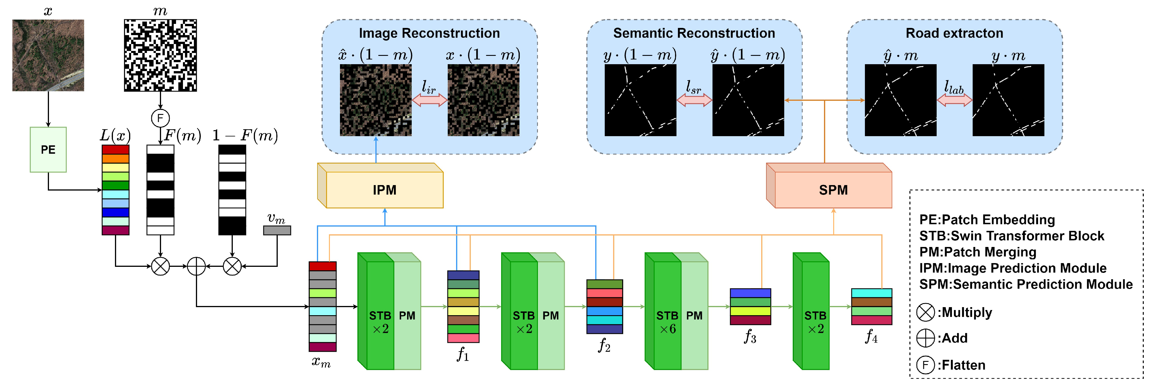
The framework of RemainNet is shown in Figure 2. As the figure shows, the network mainly contains a backbone, image prediction module (IPM), and semantic prediction module (SPM). IPM is used for RGB-wise reconstruction, thus improving low-level area feature interactions. SPM is used for semantic-wise reconstruction, thus improving high-level area feature interactions.
First, an RS image is masked according to mask m. The mask process is elaborated in the next paragraph. Then, masked image x m passes through transform blocks and generates features f 1 , f 2 , f 3 , and f 4 . Afterwards, x m , f 1 , and f 2 pass through IPM, then output reconstructed image prediction x ^ · ( 1 m ) . Finally, x m , f 1 , f 2 , f 3 , and f 4 pass through SPM, then output reconstructed semantic prediction y ^ · ( 1 m ) and road prediction y ^ · m .
The Swin Transformer blocks (STB and PM in Figure 2) [19], which are represented by green modules in the figure, are used in RemainNet. The patch embedding (PE) adopts a 4 × 4 convolutional kernel with a stride size of 4 and a flatten operation. PE embeds each 4 × 4 patch into a 1-length feature. An image embedded vector is represented by L ( x ) . F ( · ) in the figure represents the flatten operation. Mask m is randomly generated with the same size of x, and its value is 0 (masked) or 1 (unmasked). Mask m provides position information for reconstruction. The flattened mask vector F ( m ) has the same size as the image vector L ( x ) . Similar to m, the values in F ( m ) are 0 (masked) or 1 (unmasked). The masked area value v m is a learnable parameter, which has the same channel size as L ( x ) . v m automatically passes mask value information through the calculation of x m . Masked data x m are calculated according to L ( x ) , F ( m ) , and v m . Therefore, the input data x m of transformer blocks are defined as
x m = L ( x ) · F ( m ) + v m · ( 1 F ( m ) )
where x is the original RS image, m is the mask, L ( x ) is the image embedded vector, F ( m ) is the flattened mask vector.
The structure of STB (Swin Transformer block) and PM (patch merging) is shown in Figure 3. As the figure shows, STB consists of LayerNorm (LN), multilayer perceptron (MLP), window multihead self-attention (W-MSA), and shifted window multihead self-attention (SW-MSA). W-MSA computes self-attention within a window area. Each window is nonoverlapping. SW-MSA also computes self-attention within a local area, but the window in SW-MSA is overlapped with the window in W-MSA. The window self-attention extracts local self-attention within the window, thus reducing calculation complexity. The overlapped window between W-MSA and SW-MSA ensures global connection between different areas.
As the figure shows, PM is consists of flatten operation, concatenation operation, LayerNorm, and multilayer perceptron. The previous convolution encoder (like ResNet) reduces the feature size and increases the channel number by a convolution layer. Since the STB block is with a heavy weight, PM is light to change the feature size.
The masked data x m pass through transformer blocks, then generate the features f 1 , f 2 , f 3 , and f 4 from different blocks. Apart from the backbone, RemainNet contains two prediction modules, i.e., image prediction module (IPM) and semantic prediction module (SPM). IPM and SPM are used for image reconstruction and semantic segmentation, respectively.
The training losses consist of label loss l l a b , image reconstruction loss l i r , and semantic reconstruction loss l s r . The total loss l t o t a l is defined as
l t o t a l = λ m ( l i r + l s r ) + ( 1 λ m ) l l a b
where λ m is a loss weight to balance masked area loss ( l i r and l s r ) and unmasked area loss ( l l a b ).
Label loss l l a b reduces the difference between road prediction y ^ and road label y in an unmasked area. Image reconstruction loss l i r pushes image prediction of an unmasked area x ^ · ( 1 m ) to be similar to the unmasked area of an RS image x · ( 1 m ) . Semantic reconstruction loss l s r improves the similarity of semantic prediction on the masked area y ^ · ( 1 m ) and road label on the masked area y · ( 1 m ) .

3.2. Road Extraction

The unmasked area provides RS image road extraction information for a network, which is utilized by label loss l l a b . Previous road extraction methods generally use a full RS image for extracting. Since a masked image only remains part information for road extraction, the label loss on an unmasked area requires a more powerful local feature extraction ability.
Label loss is a combination of binary cross-entropy loss and dice loss. Binary cross-entropy loss pushes pixel predictions similar to corresponding labels, and it is widely used in binary semantic segmentation. Considering that road extraction faces a serious label imbalance problem, dice loss balances the dice coefficient of road and nonroad, thus alleviating the label imbalance problem. l l a b is defined as
l l a b = l b c e ( y ^ · m , y · m ) + l d i c e ( y ^ · m , y · m )
where m represents an unmasked area, y ^ is the road prediction of RemainNet, y is the road label, l b c e is binary cross entropy loss, l d i c e is dice loss. l b c e and l d i c e are defined as
l b c e ( y ^ , y ) = y · l o g ( y ^ ) ( 1 y ) l o g ( 1 y ^ )
l d i c e ( y ^ , y ) = 1 2 × | y ^ y | | y ^ | + | y |
where | · | denotes calculating the sum of pixel values, and y ^ y denotes the intersection of y ^ and y.

3.3. Image Reconstruction

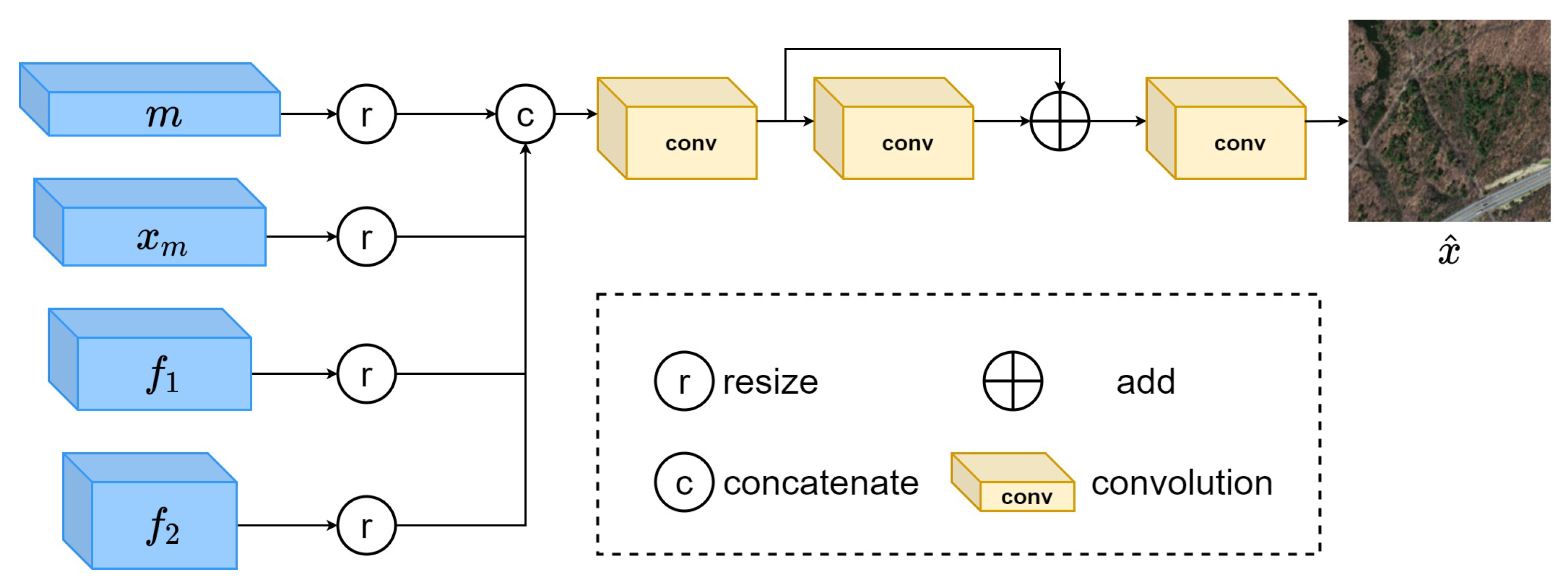
The structure of IPM is shown in Figure 4. IPM takes x m , f 1 , and f 2 as inputs, then generates image prediction x ^ . Since the input of IPM contains shallow layer features and the output value represents an RGB value in a reconstructed area, image reconstruction encourages low-level (RGB-wise) area information interactions. Thus, the occluded area features are connected with other areas. Most previous MIM methods [58,60] directly reconstruct an image by high-level features, i.e., the downstream target representations, resulting in representation mismatching between pretraining and training. In order to reduce representation mismatching, we only use shallow features for image reconstruction.
In order to reconstruct an image masked area at the RGB level, IPM inputs low-level features x m , f 1 , and f 2 . The features provide different low-level information for image reconstruction. The masked areas in a reconstructed image and original RS image are ought to be similar. Thus, image reconstruction loss l i r is used to reduce the above difference. Like many image regression works, we adopt L1 loss for reconstructing a masked area. l i r is defined as
l i r = | x ^ · ( 1 m ) x · ( 1 m ) | 1
where 1 m represents a masked area, x ^ is image prediction, x is the original RS image, and | · | 1 represents L1 loss.

3.4. Semantic Reconstruction

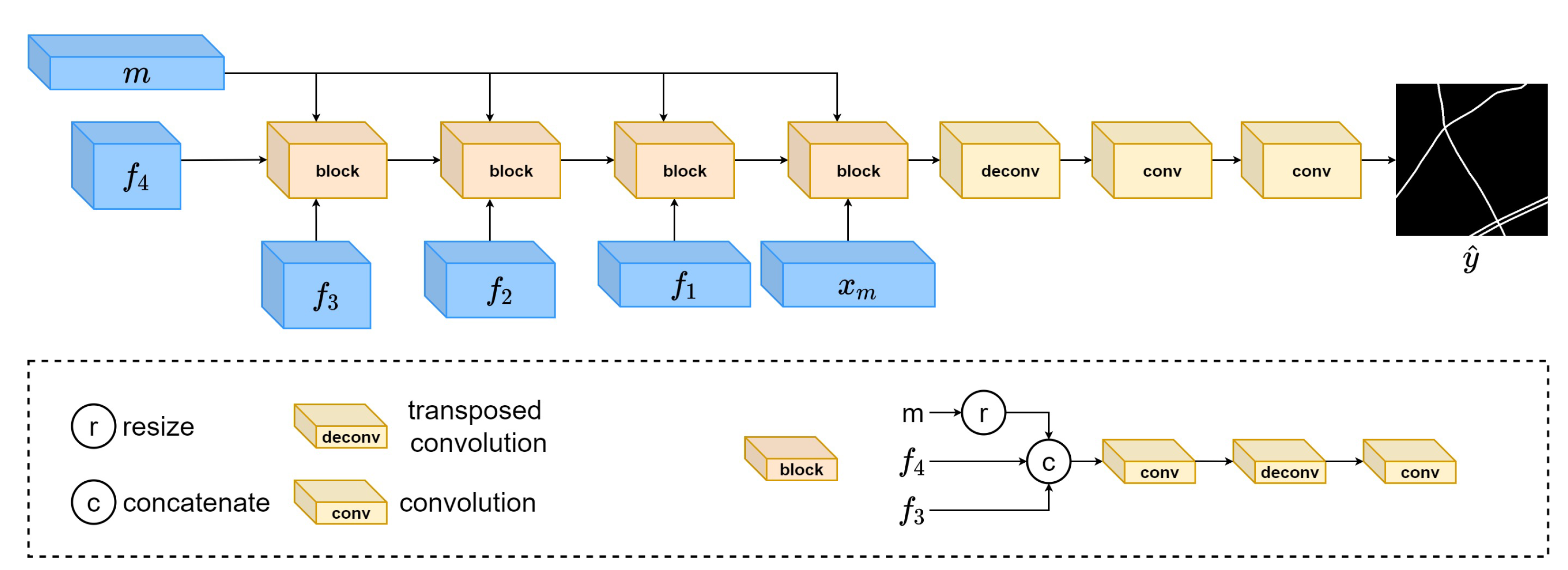
The structure of SPM is shown in Figure 5. SPM takes x m , f 1 , f 2 , f 3 , and f 4 as input, then generates road prediction y ^ . Semantic reconstruction encourages a network to infer masked area roads from RS image unmasked areas. Since f 3 and f 4 have passed through numerous transformer layers and the reconstruction is semantic-wise, semantic reconstruction improves high-level area information interactions. Most previous MIM methods [58,60] do not utilize label information because they focus on self-supervised learning. Since the road label is provided in the experiment, and multitask learning with similar semantics in features has proven to be beneficial [12], we adopt semantic reconstruction to enforce high-level semantic interactions of different areas.
Previous MIM methods mainly reconstruct an original image, since they are mainly used to unsupervise pretraining. However, image reconstruction is RGB-wise reconstruction rather than semantic-wise reconstruction. Since road labels are available, and our final target is improving road prediction accuracy of occluded areas, we propose semantic reconstruction to increase semantic-wise interactions. The goal of semantic reconstruction is to use unmasked area information to infer a road in masked areas.
Compared with image reconstruction, the task is more challenging. Image reconstruction can be inferred by nearby pixel RGB values, since the RGB distribution is generally close in most places and the input provides RGB values of an unmasked area. Semantic reconstruction can also be inferred by nearby semantic labels. However, the labels are not provided in the input, and the road label faces a label imbalance problem; thus, the nearby road provides less information, and the road label is not as continuous as the RGB value.
Similar to image reconstruction, we adopt SPM for semantic reconstruction. The inputs of SPM are x m , f 1 , f 2 , f 3 , and f 4 , which contain high-level features. The masked area road prediction using unmasked area information is pushed to be similar with road labels by semantic reconstruction loss l s r . The semantic reconstruction adopts binary cross-entropy loss. The designed semantic reconstruction loss l s r is defined as
l s r = l b c e ( y ^ · ( 1 m ) , y · ( 1 m ) )
where y ^ is road prediction, and y is road label.

4. Experiments

4.1. Dataset

We conducted experiments on the Massachusetts Roads dataset [67] and DeepGlobe Road Extraction dataset [68]. The brief information is listed in Table 1. The details of the datasets are follows:
(1)
The Massachusetts Roads dataset contains 1171 RS images with labels, including 1108 training images, 14 validation images, and 49 test images. The dataset covers around 2600 sq. km area with a resolution of 120 cm/pixel. The original size of each image is 1500 × 1500. We resize them, then crop them into the size of 512 × 512 without overlapping; thus, the training, validation, and test image numbers are 9972, 126, and 441, respectively.
(2)
The DeepGlobe Road Extraction dataset consists of 8570 RS images, including 6226 satellite images with labels and 2344 RS images without labels. The dataset covers around 2220 sq. km area with a resolution of 50 cm/pixel. The size of each image is 1024 × 1024. In the experiment, we resize 6226 RS images with labels into 512 × 512, then randomly divide them into subsets with a rate of 0.8 (training set), 0.1 (validation set), and 0.1 (test set).
Table 1. Brief information of the datasets used in the experiment.
DatasetTrainingValidationTestTotal
Massachusetts Roads997212644110,539
DeepGlobe Road Extraction49826226226226

4.2. Baselines and Metrics

To verify the effectiveness of the proposed RemainNet, some state-of-the-art methods are selected:
(1)
DeepLab v3+ [27]. DeepLab v3+ is a classical semantic segmentation model, which employs an encoder–decoder structure with atrous convolution. The encoder encodes multiscale contextual information, and the decoder is simple yet effective.
(2)
D-LinkNet [49]. D-LinkNet is a classical road extraction model, which is built on a LinkNet architecture. It contains dilated convolution layers to expand a receptive field. The network had the best IoU scores in the CVPR DeepGlobe 2018 Road Extraction Challenge.
(3)
NL-LinkNet [10]. NL-LinkNet is the first RS image road extraction model to use nonlocal operations. The nonlocal block ensures the model to capture long-range dependencies and distant information.
(4)
MACU-Net [38]. MACU-Net is based on U-Net. MACU-Net employs a multiscale skip connection and asymmetric convolution block for a higher feature extract ability.
(5)
RoadExNet [13]. RoadExNet is the generator of SemiRoadExNet. RoadExNet employs a vertical attention module and horizontal attention module to concentrate on road areas.
The evaluation metrics used in the experiment are precision (P), recall (R), F1-score (F1), and intersection over union (IoU). The evaluation matrices are formulated as follows:
P = T P T P + F P
R = T P T P + T N
F 1 = 2 × P × R P + R
I o U = T P T P + F P + F N
where TP, FP, TN, and FN are the number of true positives, false positives, true negatives, and false negatives, respectively.

4.3. Implementation Details

The experiments are conducted with a PyTorch framework on a single NVIDIA RTX 3080 GPU. We adopt AdamW as the parameter optimizer. The learning rate is set as 2 × 10 4 initially. We adopt polynomial learning rate decay: ( 1 i t e r m a x i t e r ) 0.9 . The weight decay of the AdamW optimizer is set as 1 × 10 4 . The training epoch number is set as 150. The batch size is set as 12. The mask patch size is set as and 16 × 16 . The mask rate is set as 0.75 initially, and it linearly reduces to 0 in the 100th epoch. The loss weight λ m is equal to the mask rate. In order to improve network generalization, we adopt random crop, random flip, random rotation, random affine, random color jitter, random gray, and Gaussian blur for data augmentation.

4.4. Experimental Result

4.4.1. Results in Massachusetts Roads Dataset

The road extraction results on the Massachusetts Roads dataset are detailed in Table 2. As the table shows, the proposed RemainNet gains the highest F1 (0.7872) and IoU (0.6491). DeepLab v3+ achieves the highest precision (0.8391) but the lowest F1 and lowest IoU. This result reflects that DeepLab v3+ tends to predict a nonroad label, which means that the label imbalance problem is not solved well. D-LinkNet achieves the highest recall (0.7681) but the worst precision. The result reveals that D-LinkNet tends to predict a road in indiscernible areas. However, the precision of RemainNet is not high like recall, F1, and IoU. The occlusion areas of the road is generally more than areas that are similar to a road; i.e., an occluded road is more likely to be misjudged as a nonroad compared with a nonroad misjudged as a road (seen in Figure 6). MIM encourages the context inference of occluded areas; thus, more nonroad areas are misjudged as road areas.
RemainNet obtains 1.75% higher F1 and 2.34% higher IoU than DeepLab v3+, which reflects quite a high difference. D-LinkNet has modest performance but still obtains 0.76% lower F1 and 1.04% lower IoU. Compared with NL-LinkNet, RemainNet obtains 0.89% higher IoU, which indicates stronger area interactions with MIM. RoadExNet achieves the second-highest F1 and the second-highest IoU, only 0.60% lower F1 and 0.82% lower IoU. DeepLab v3+ and D-LinkNet tend to enlarge the receptive field. A larger receptive field means more context information to some extent, but they ignore the improved network-self information extraction ability. NL-LinkNet, MACU-Net, and RoadExNet notice the importance of the information extraction ability; thus, they use an attention mechanism to extract nonlocal information.These methods alleviate the occlusion problem by a stronger information extraction ability, but they do not further improve the inference ability of occluded areas. RemainNet introduces the masking and reconstructing process, thus improving the inference ability of occluded areas.
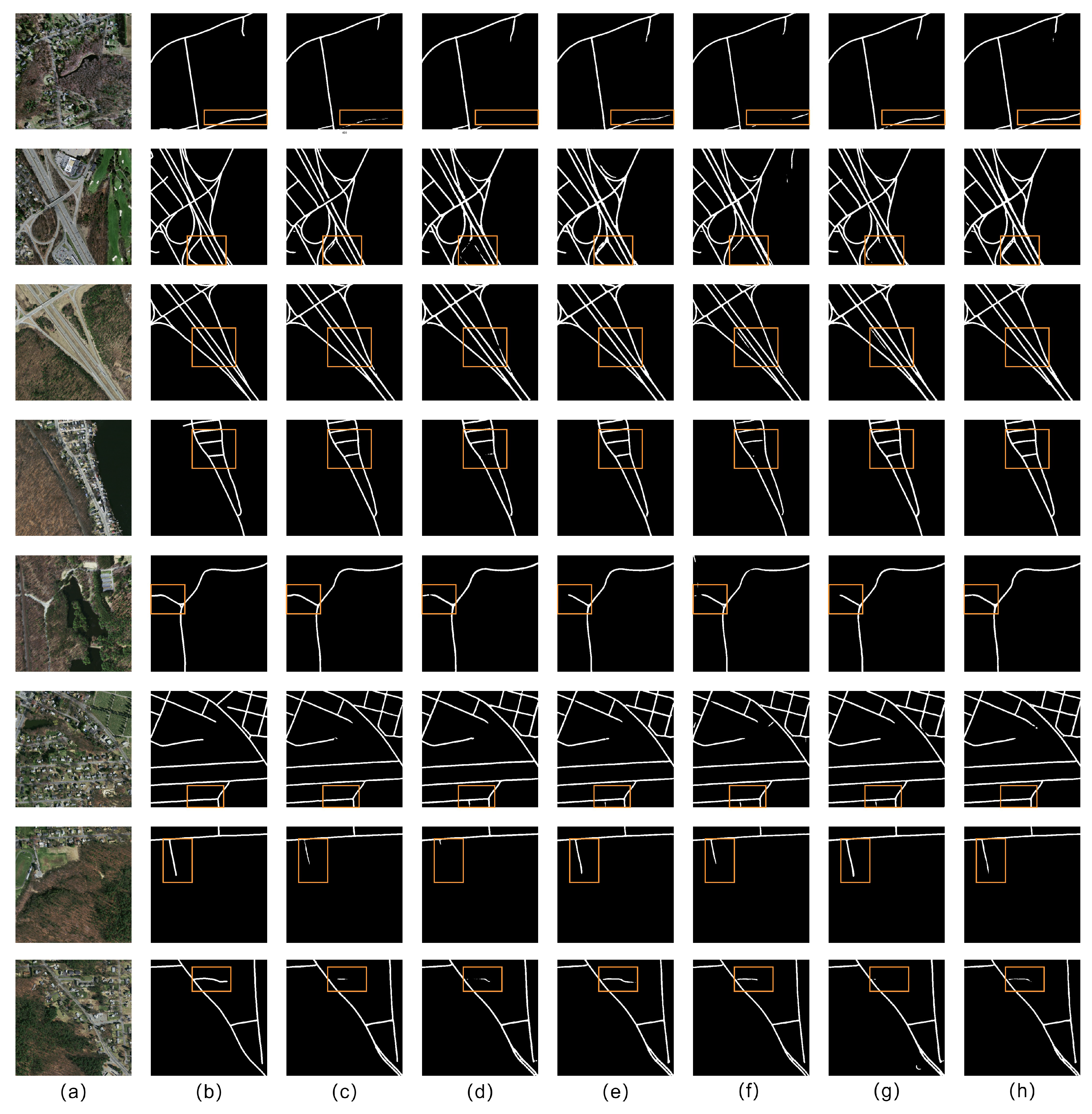
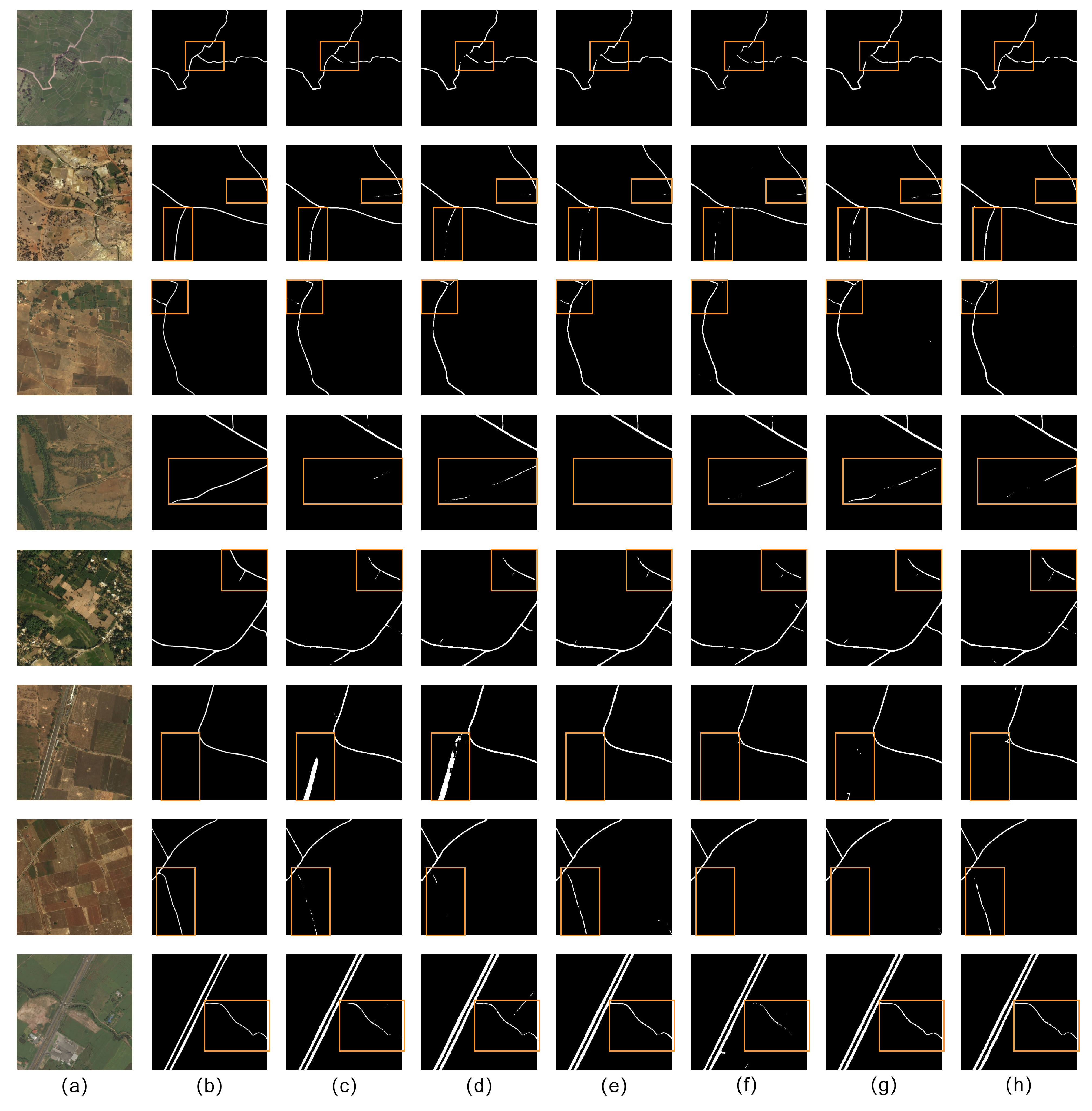
The visual road extraction results are shown in Figure 6. In the first row, the road on the bottom is obstructed by trees and shallows. The predictions of DeepLab v3+, D-LinkNet, and MACU-Net in the first row miss an obstructed road. In the second row, the parking lot is with a similar visual feature as a road; thus, DeepLab v3+, MACU-Net, and RoadExNet are not able to distinguish. The roads in the third row are with a different width; D-LinkNet misses a little road. The road in the fourth-row box is short and occluded by trees; D-LinkNet and MACU-Net miss the road. The road in the fifth row is blocked by a train track, but DeepLab v3+ and RemainNet still predict well. The road in the image edge is short, reflecting that local discrimination is also important. The sixth row reveals that some methods mislead by the building. Two roads in the seventh row are interrupted by trees; thus, D-LinkNet misses the road. In the last row, the main road has a different feature with a lane; thus, some methods gain wrong predictions. The above observations concentrate on confusible areas. Besides, the discontinuity of RemainNet prediction is lower compared with other methods. Generally, the proposed RemainNet achieves the best visual results especially in occluded areas.

4.4.2. Results in DeepGlobe Road Extraction Dataset

Table 3 shows road extraction results on the DeepGlobe Road Extraction dataset. As the table reflects, the proposed RemainNet achieves the highest recall (0.7942), F1 (0.7816), and IoU (0.6415). MACU-Net achieves the highest precision (0.7893) but the lowest recall, which indicates that MACU-Net tends to generate nonroad prediction.
Compared with DeepLab v3+, RemainNet gains 1.27% higher F1 and 1.70% higher IoU. D-LinkNet achieves the second-highest recall, but it remains a 0.84% lower recall. NL-LinkNet achieves the third-lowest IoU; thus, RemainNet achieves 1.93% higher F1 and 2.56% higher IoU than NL-LinkNet. MACU-Net achieves 1.99% higher precision but 8.19% lower recall than RemainNet. Besides, the F1 and IoU of MACU-Net is lowest. The recall is 3.87% higher than precision in RoadExNet, indicating that RoadExNet also tends to extracts the road. The F1 and IoU of MACU-Net are 2.00% and 2.66% lower than RemainNet, respectively.
Figure 7 shows the visual results of the DeepGlobe Road Extraction dataset. In the first row, some trees cover the road; thus DeepLab v3+, D-LinkNet, and MACU-Net predictions are discontinuous in the place. In the second row, the background and road are similar, but RemainNet prediction remains the most similar with a road label. The road in the third-row box is hard to distinguish, because the road is in the image edge place and some trees occlude the road. However, NL-LinkNet, RoadExNet, and RemainNet still predict well. The road in the fourth row is not the main road, and it connects a river; thus, all methods predict inaccurately, especially DeepLab v3+ and NL-LinkNet. In the fifth row, trees are dense on both sides of the road; thus, the predictions in DeepLab v3+, D-LinkNet, MACU-Net, and RoadExNet are imprecise. The train track in the sixth row also has a linear shape, resulting in wrong predictions in the sixth row. In the seventh row, the road color is very similar to the background, and a bent lane is around it. NL-LinkNet and RemainNet have a stronger nonlocal distinguishment; thus, the predictions are more accurate. In the last row, the road is around the river, and their shapes are similar, but NL-LinkNet, RoadExNet, and RemainNet obtain similar results as a road label. Overall, RemainNet achieves the best visual result.

4.4.3. Comparison of Parameters and Computational Complexity

Table 4 details FLOPs per image and a network parameter. As for FLOPS, NL-LinkNet achieves the lowest FLOPs and DeepLab v3+ achieves the highest FLOPs. The proposed RemainNet achieves the second-highest calculation. RemainNet introduces image reconstruction, which increases calculation burden. As for parameters, MACU-Net achieves the lowest parameters, and DeepLab v3+ achieves the highest parameters. The parameter of RemainNet is slightly higher than D-LinkNet and RoadExNet, but smaller than DeepLab v3+. Considering that RemainNet has an extra module for image reconstruction, the parameter of RemainNet is modest.

4.5. Ablation Study

In order to explore the influence of image reconstruction (IR) and semantic reconstruction (SR), we conduct ablation experiments on RemainNet. As Table 5 shows, a network with IR and SR achieves the best recall, F1 and IoU in two datasets. RemainNet without IR and SR gains the highest precision (0.8126) but worst recall (0.7541) in the Massachusetts Roads dataset. The difference reveals that SR and IR encourage occluded areas to conduct road prediction with context information. Notably, F1 and IoU in RemainNet without IR are a little higher than RemainNet without SR. IR and SR both encourage area interactions, but SR is a more challenging task; thus, SR needs feature-level context information. The performance without IR/SR is worse than RemainNet, confirming that IR and SR are both beneficial for road extraction.

5. Discussion

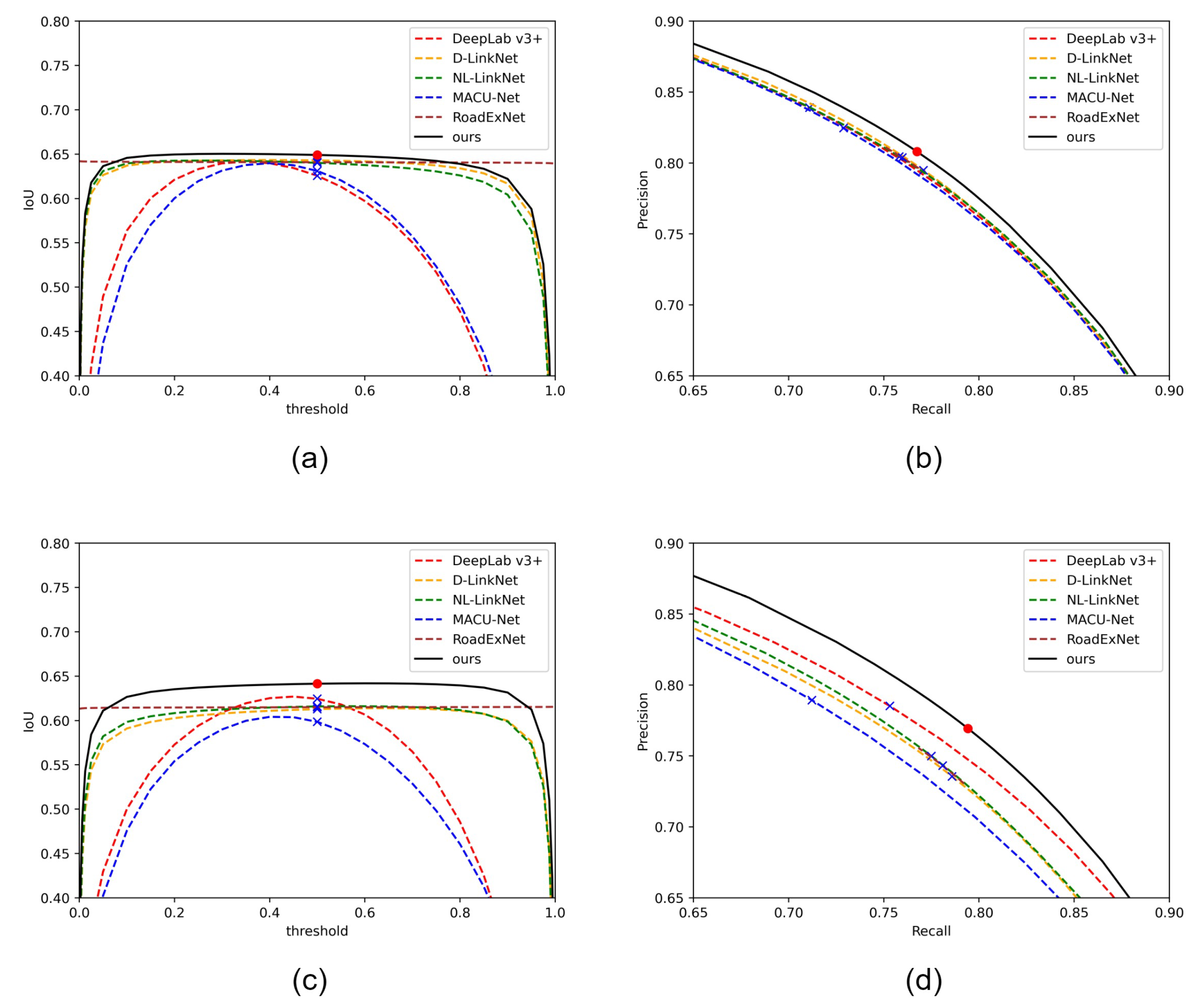
Figure 8 shows the accuracy curves of different methods. As Figure 8a,c show, the IoU of RemainNet (black line) generally changes little when the road threshold changes, which indicates fine robustness. The IoU of DeepLab v3+ and MACU-Net changes more with the threshold changes, indicating worse robustness. Figure 8b,d are the precision–recall curves of different methods. The precision–recall curves of RemainNet generally wrap around the precision–recall curves of other methods, reflecting a better road extraction performance of RemainNet. Since the road in the Massachusetts Roads dataset is with the same width but the road in the DeepGlobe Road Extraction dataset is not, the performance difference is more obvious in (d) than in (b).
In the experiment, the mask rate is linearly reduced from 0.75 to 0. Previous MIM methods only used image unmasked area reconstruction in the pretraining period, and the mask rate is fixed. Besides, previous works [58,60] find that a high mask rate can obtain good performance, because a high mask rate means a strong information interaction with long-range areas. Our method introduces semantic reconstruction in the first period and only conducts road extraction in the latter period. Therefore, we think that the linearly reduced mask rate can ensure a smooth transition. Therefore, we conduct an experiment about mask strategy, and the result is shown in Table 6. In the table, ‘keep unchanging(0.75)’ means that the mask rate keeps 0.75, ‘keep unchanging(0.375)’ means that the mask rate keeps 0.375, ‘linearly reduce’ means that the mask rate linearly reduces to 0. As the table shows, a linearly reduced mask rate generally obtains a silently better performance. As Formula (2) shows, road extraction is involved in the earlier period; thus, a linearly reduced masked rate means a linearly increased road extraction. Besides, a linearly reduced mask rate increases the weight of the road extraction gradually.
The image reconstruction results are shown in Figure 9. Since the training is just starting in the firth epoch, and the MIM training is ending in the 100th epoch, we use the 50th epoch weight for image reconstruction. In the figure, images in the first to the third row are from the Massachusetts Roads dataset, and images in the fourth to the last row are from the DeepGlobe Road Extraction dataset. The first and the fourth rows are a rural area with many trees. The second and the fifth rows are suburbs with sparse building. The third and the last rows are cities. Generally, the reconstructed areas are roughly similar to the original image in visual effect. Since the reconstructed image only uses half-area information of the original image, the result reflects that RemainNet learns the connections of different areas. Besides, the reconstructed images in a rural area achieve the best visual results, while the image in cities achieves the worst. Since a large mask rate leads to much information lost, some complex area is hard to reconstruct. The results in previous works [58] also reflect this point. The rural area is more simple with much redundancy information; thus, its reconstructed results are closer to the original image.

6. Conclusions

In this paper, we propose a novel road extraction network named RemainNet in order to mitigate the impact of occlusions. The major contribution of the paper is, first, exploring and alleviating the occlusion problem by MIM. RemainNet infers the occluded area by context information, and the inference ability is enforced by inferring the masked area information from unmasked areas. The RS image is masked first; then the RGB values of the masked area are inferred by IPM. Apart from image reconstruction, we also develop semantic reconstruction by SPM. We have verified the effectiveness of RemainNet through numerous comparative experiments and ablation experiments on two public road extraction datasets. The results indicate that the proposed RemainNet outperforms other state-of-the-art road extraction methods. In the future, we plan to focus on road extraction using 3-D data in order to obtain more practical application for our daily life.

Author Contributions

Conceptualization, methodology, investigation, data curation, formal analysis, and writing—original draft preparation, Z.L.; conceptualization, methodology, investigation, and writing—review and editing, H.C. Supervision, H.C., N.J. and J.L. All the authors read, edited, and critiqued the manuscript and approved the final version.All authors have read and agreed to the published version of the manuscript.

Funding

This research was jointly supported by the National NSF of China under Grant No. U19A2058, No. 41971362, No. 41871248, and No. 62106276.

Institutional Review Board Statement

Not applicable.

Informed Consent Statement

Not applicable.

Data Availability Statement

This study did not report any data.

Acknowledgments

The authors would also like to thank the anonymous referees for their valuable comments and helpful suggestions.

Conflicts of Interest

The authors declare no conflict of interest.

References

  1. Abdollahi, A.; Pradhan, B.; Shukla, N.; Chakraborty, S.; Alamri, A. Deep learning approaches applied to remote sensing datasets for road extraction: A state-of-the-art review. Remote Sens. 2020, 12, 1444. [Google Scholar] [CrossRef]
  2. Zi, W.; Xiong, W.; Chen, H.; Li, J.; Jing, N. SGA-Net: Self-constructing graph attention neural network for semantic segmentation of remote sensing images. Remote Sens. 2021, 13, 4201. [Google Scholar] [CrossRef]
  3. Song, J.; Chen, H.; Du, C.; Li, J. Semi-MapGen: Translation of Remote Sensing Image into Map via Semi-supervised Adversarial Learning. IEEE Trans. Geosci. Remote. Sens. 2023, 61, 4701219. [Google Scholar] [CrossRef]
  4. Zi, W.; Xiong, W.; Chen, H.; Chen, L. TAGCN: Station-level demand prediction for bike-sharing system via a temporal attention graph convolution network. Inf. Sci. 2021, 561, 274–285. [Google Scholar] [CrossRef]
  5. Lian, R.; Wang, W.; Mustafa, N.; Huang, L. Road extraction methods in high-resolution remote sensing images: A comprehensive review. IEEE J. Sel. Top. Appl. Earth Obs. Remote Sens. 2020, 13, 5489–5507. [Google Scholar] [CrossRef]
  6. Feng, S.; Ji, K.; Wang, F.; Zhang, L.; Ma, X.; Kuang, G. PAN: Part Attention Network Integrating Electromagnetic Characteristics for Interpretable SAR Vehicle Target Recognition. IEEE Trans. Geosci. Remote Sens. 2023, 61, 5204617. [Google Scholar] [CrossRef]
  7. Wu, S.; Du, C.; Chen, H.; Xu, Y.; Guo, N.; Jing, N. Road extraction from very high resolution images using weakly labeled OpenStreetMap centerline. ISPRS Int. J. Geo-Inf. 2019, 8, 478. [Google Scholar] [CrossRef]
  8. Chen, H.; Peng, S.; Du, C.; Li, J.; Wu, S. SW-GAN: Road Extraction from Remote Sensing Imagery Using Semi-Weakly Supervised Adversarial Learning. Remote Sens. 2022, 14, 4145. [Google Scholar] [CrossRef]
  9. Mei, J.; Li, R.J.; Gao, W.; Cheng, M.M. CoANet: Connectivity attention network for road extraction from satellite imagery. IEEE Trans. Image Process. 2021, 30, 8540–8552. [Google Scholar] [CrossRef]
  10. Wang, Y.; Seo, J.; Jeon, T. NL-LinkNet: Toward lighter but more accurate road extraction with nonlocal operations. IEEE Geosci. Remote Sens. Lett. 2021, 19, 3000105. [Google Scholar] [CrossRef]
  11. Chen, S.B.; Ji, Y.X.; Tang, J.; Luo, B.; Wang, W.Q.; Lv, K. DBRANet: Road extraction by dual-branch encoder and regional attention decoder. IEEE Geosci. Remote Sens. Lett. 2021, 19, 3002905. [Google Scholar] [CrossRef]
  12. Li, R.; Gao, B.; Xu, Q. Gated auxiliary edge detection task for road extraction with weight-balanced loss. IEEE Geosci. Remote Sens. Lett. 2020, 18, 786–790. [Google Scholar] [CrossRef]
  13. Chen, H.; Li, Z.; Wu, J.; Xiong, W.; Du, C. SemiRoadExNet: A semi-supervised network for road extraction from remote sensing imagery via adversarial learning. ISPRS J. Photogramm. Remote Sens. 2023, 198, 169–183. [Google Scholar] [CrossRef]
  14. Wei, Y.; Zhang, K.; Ji, S. Simultaneous road surface and centerline extraction from large-scale remote sensing images using CNN-based segmentation and tracing. IEEE Trans. Geosci. Remote Sens. 2020, 58, 8919–8931. [Google Scholar] [CrossRef]
  15. Xu, Y.; Chen, H.; Du, C.; Li, J. MSACon: Mining spatial attention-based contextual information for road extraction. IEEE Trans. Geosci. Remote Sens. 2021, 60, 5604317. [Google Scholar] [CrossRef]
  16. Ding, L.; Bruzzone, L. DiResNet: Direction-aware residual network for road extraction in VHR remote sensing images. IEEE Trans. Geosci. Remote Sens. 2020, 59, 10243–10254. [Google Scholar] [CrossRef]
  17. Yang, Z.; Zhou, D.; Yang, Y.; Zhang, J.; Chen, Z. Road Extraction From Satellite Imagery by Road Context and Full-Stage Feature. IEEE Geosci. Remote. Sens. Lett. 2022, 20, 8000405. [Google Scholar] [CrossRef]
  18. Li, S.; Wu, D.; Wu, F.; Zang, Z.; Sun, B.; Li, H.; Xie, X.; Li, S. Architecture-Agnostic Masked Image Modeling–From ViT back to CNN. arXiv 2022, arXiv:2205.13943. [Google Scholar]
  19. Liu, Z.; Lin, Y.; Cao, Y.; Hu, H.; Wei, Y.; Zhang, Z.; Lin, S.; Guo, B. Swin transformer: Hierarchical vision transformer using shifted windows. In Proceedings of the IEEE/CVF International Conference on Computer Vision, Montreal, QC, Canada, 10–17 October 2021; pp. 10012–10022. [Google Scholar]
  20. Khan, S.H.; Bennamoun, M.; Sohel, F.; Togneri, R. Geometry driven semantic labeling of indoor scenes. In European Conference on Computer Vision; Springer: Berlin/Heidelberg, Germany, 2014; pp. 679–694. [Google Scholar]
  21. Jaiswal, S.; Pandey, M. A Review on Image Segmentation. Rising Threat. Expert Appl. Solut. 2021, 2020, 233–240. [Google Scholar]
  22. Yuan, X.; Shi, J.; Gu, L. A review of deep learning methods for semantic segmentation of remote sensing imagery. Expert Syst. Appl. 2021, 169, 114417. [Google Scholar] [CrossRef]
  23. Long, J.; Shelhamer, E.; Darrell, T. Fully convolutional networks for semantic segmentation. In Proceedings of the IEEE Conference on Computer Vision and Pattern Recognition, Vancouver, BC, Canada, 17–24 June 2023; pp. 3431–3440. [Google Scholar]
  24. Ronneberger, O.; Fischer, P.; Brox, T. U-net: Convolutional networks for biomedical image segmentation. In Proceedings of the Medical Image Computing and Computer-Assisted Intervention–MICCAI 2015: 18th International Conference, Munich, Germany, 5–9 October 2015; Proceedings, Part III 18. Springer: Berlin/Heidelberg, Germany, 2015; pp. 234–241. [Google Scholar]
  25. Badrinarayanan, V.; Kendall, A.; Cipolla, R. Segnet: A deep convolutional encoder-decoder architecture for image segmentation. IEEE Trans. Pattern Anal. Mach. Intell. 2017, 39, 2481–2495. [Google Scholar] [CrossRef]
  26. Chen, L.C.; Papandreou, G.; Kokkinos, I.; Murphy, K.; Yuille, A.L. Deeplab: Semantic image segmentation with deep convolutional nets, atrous convolution, and fully connected crfs. IEEE Trans. Pattern Anal. Mach. Intell. 2017, 40, 834–848. [Google Scholar] [CrossRef] [PubMed]
  27. Chen, L.C.; Zhu, Y.; Papandreou, G.; Schroff, F.; Adam, H. Encoder-decoder with atrous separable convolution for semantic image segmentation. In Proceedings of the European Conference on Computer Vision (ECCV), Munich, Germany, 8–14 September 2018; pp. 801–818. [Google Scholar]
  28. Ulku, I.; Akagündüz, E. A survey on deep learning-based architectures for semantic segmentation on 2d images. Appl. Artif. Intell. 2022, 36, 2032924. [Google Scholar] [CrossRef]
  29. Dosovitskiy, A.; Beyer, L.; Kolesnikov, A.; Weissenborn, D.; Zhai, X.; Unterthiner, T.; Dehghani, M.; Minderer, M.; Heigold, G.; Gelly, S.A. An Image is Worth 16 × 16 Words: Transformers for Image Recognition at Scale. In Proceedings of the International Conference on Learning Representations, Virtual Event, 3–7 May 2021. [Google Scholar]
  30. Lv, P.; Wu, W.; Zhong, Y.; Zhang, L. Review of Vision Transformer Models for Remote Sensing Image Scene Classification. In Proceedings of the IGARSS 2022—2022 IEEE International Geoscience and Remote Sensing Symposium, Kuala Lumpur, Malaysia, 17–22 July 2022; pp. 2231–2234. [Google Scholar] [CrossRef]
  31. Han, K.; Wang, Y.; Chen, H.; Chen, X.; Guo, J.; Liu, Z.; Tang, Y.; Xiao, A.; Xu, C.; Xu, Y.; et al. A Survey on Vision Transformer. IEEE Trans. Pattern Anal. Mach. Intell. 2023, 45, 87–110. [Google Scholar] [CrossRef] [PubMed]
  32. Touvron, H.; Cord, M.; Douze, M.; Massa, F.; Sablayrolles, A.; Jegou, H. Training data-efficient image transformers & distillation through attention. In Proceedings of the 38th International Conference on Machine Learning, Virtual Event, 18–24 July 2021; Meila, M., Zhang, T., Eds.; Volume 139, pp. 10347–10357. [Google Scholar]
  33. Chu, X.; Tian, Z.; Zhang, B.; Wang, X.; Wei, X.; Xia, H.; Shen, C. Conditional Positional Encodings for Vision Transformers. arXiv 2021, arXiv:2102.10882. [Google Scholar]
  34. Li, Y.; Zhang, K.; Cao, J.; Timofte, R.; Gool, L.V. LocalViT: Bringing Locality to Vision Transformers. arXiv 2021, arXiv:2104.05707. [Google Scholar]
  35. Strudel, R.; Garcia, R.; Laptev, I.; Schmid, C. Segmenter: Transformer for Semantic Segmentation. In Proceedings of the IEEE/CVF International Conference on Computer Vision (ICCV), Paris, France, 2–6 October 2021; pp. 7262–7272. [Google Scholar]
  36. Xie, E.; Wang, W.; Yu, Z.; Anandkumar, A.; Alvarez, J.M.; Luo, P. SegFormer: Simple and Efficient Design for Semantic Segmentation with Transformers. In Advances in Neural Information Processing Systems; Beygelzimer, A., Dauphin, Y., Liang, P., Vaughan, J.W., Eds.; IEEE: Piscataway Township, NJ, USA, 2021. [Google Scholar]
  37. Jin, Y.; Han, D.; Ko, H. TrSeg: Transformer for semantic segmentation. Pattern Recognit. Lett. 2021, 148, 29–35. [Google Scholar] [CrossRef]
  38. Li, R.; Duan, C.; Zheng, S.; Zhang, C.; Atkinson, P.M. MACU-Net for Semantic Segmentation of Fine-Resolution Remotely Sensed Images. IEEE Geosci. Remote. Sens. Lett. 2021, 19, 8007205. [Google Scholar] [CrossRef]
  39. Wan, Q.; Huang, Z.; Lu, J.; Yu, G.; Zhang, L. SeaFormer: Squeeze-enhanced Axial Transformer for Mobile Semantic Segmentation. arXiv 2023, arXiv:2301.13156. [Google Scholar]
  40. Yuan, F.; Zhang, Z.; Fang, Z. An effective CNN and Transformer complementary network for medical image segmentation. Pattern Recognit. 2023, 136, 109228. [Google Scholar] [CrossRef]
  41. Chen, Z.; Deng, L.; Luo, Y.; Li, D.; Marcato Junior, J.; Nunes Gonçalves, W.; Awal Md Nurunnabi, A.; Li, J.; Wang, C.; Li, D. Road extraction in remote sensing data: A survey. Int. J. Appl. Earth Obs. Geoinf. 2022, 112, 102833. [Google Scholar] [CrossRef]
  42. Sghaier, M.O.; Lepage, R. Road extraction from very high resolution remote sensing optical images based on texture analysis and beamlet transform. IEEE J. Sel. Top. Appl. Earth Obs. Remote Sens. 2015, 9, 1946–1958. [Google Scholar] [CrossRef]
  43. Wang, J.; Qin, Q.; Yang, X.; Wang, J.; Ye, X.; Qin, X. Automated road extraction from multi-resolution images using spectral information and texture. In Proceedings of the 2014 IEEE Geoscience and Remote Sensing Symposium, Quebec City, QC, Canada, 13–18 July 2014; IEEE: Piscataway Township, NJ, USA, 2014; pp. 533–536. [Google Scholar]
  44. He, C.; Liao, Z.x.; Yang, F.; Deng, X.p.; Liao, M.s. Road extraction from SAR imagery based on multiscale geometric analysis of detector responses. IEEE J. Sel. Top. Appl. Earth Obs. Remote Sens. 2012, 5, 1373–1382. [Google Scholar] [CrossRef]
  45. Wei, Y.; Wang, Z.; Xu, M. Road structure refined CNN for road extraction in aerial image. IEEE Geosci. Remote Sens. Lett. 2017, 14, 709–713. [Google Scholar] [CrossRef]
  46. Abdollahi, A.; Pradhan, B.; Shukla, N. Extraction of road features from UAV images using a novel level set segmentation approach. Int. J. Urban Sci. 2019, 23, 391–405. [Google Scholar] [CrossRef]
  47. Xin, J.; Zhang, X.; Zhang, Z.; Fang, W. Road extraction of high-resolution remote sensing images derived from DenseUNet. Remote Sens. 2019, 11, 2499. [Google Scholar] [CrossRef]
  48. Abdollahi, A.; Pradhan, B.; Sharma, G.; Maulud, K.N.A.; Alamri, A. Improving road semantic segmentation using generative adversarial network. IEEE Access 2021, 9, 64381–64392. [Google Scholar] [CrossRef]
  49. Zhou, L.; Zhang, C.; Wu, M. D-LinkNet: LinkNet with pretrained encoder and dilated convolution for high resolution satellite imagery road extraction. In Proceedings of the IEEE Conference on Computer Vision and Pattern Recognition Workshops, Salt Lake City, UT, USA, 8–23 June 2018; pp. 182–186. [Google Scholar]
  50. Abdollahi, A.; Bakhtiari, H.R.R.; Nejad, M.P. Investigation of SVM and level set interactive methods for road extraction from google earth images. J. Indian Soc. Remote Sens. 2018, 46, 423–430. [Google Scholar] [CrossRef]
  51. Tao, C.; Qi, J.; Li, Y.; Wang, H.; Li, H. Spatial information inference net: Road extraction using road-specific contextual information. ISPRS J. Photogramm. Remote Sens. 2019, 158, 155–166. [Google Scholar] [CrossRef]
  52. Zhou, Q.; Yu, C.; Luo, H.; Wang, Z.; Li, H. MimCo: Masked Image Modeling Pre-training with Contrastive Teacher. In Proceedings of the 30th ACM International Conference on Multimedia, Lisboa, Portugal, 10–14 October 2022; pp. 4487–4495. [Google Scholar]
  53. Radford, A.; Narasimhan, K.; Salimans, T.; Sutskever, I. Improving Language Understanding by Generative Pre-Training; 2018; p. 12. Available online: https://s3-us-west-2.amazonaws.com/openai-assets/research-covers/language-unsupervised/language_understanding_paper.pdf (accessed on 20 June 2023).
  54. Devlin, J.; Chang, M.W.; Lee, K.; Toutanova, K. Bert: Pre-training of deep bidirectional transformers for language understanding. arXiv 2018, arXiv:1810.04805. [Google Scholar]
  55. Chen, M.; Radford, A.; Child, R.; Wu, J.; Jun, H.; Luan, D.; Sutskever, I. Generative pretraining from pixels. In Proceedings of the International Conference on Machine Learning, Virtual Event, 13–18 July 2020; pp. 1691–1703. [Google Scholar]
  56. Bao, H.; Dong, L.; Wei, F. BEiT: BERT Pre-Training of Image Transformers. arXiv 2021, arXiv:2106.08254. [Google Scholar]
  57. Caron, M.; Touvron, H.; Misra, I.; Jégou, H.; Mairal, J.; Bojanowski, P.; Joulin, A. Emerging properties in self-supervised vision transformers. In Proceedings of the IEEE/CVF International Conference on Computer Vision, Montreal, QC, Canada, 10–17 October 2021; pp. 9650–9660. [Google Scholar]
  58. He, K.; Chen, X.; Xie, S.; Li, Y.; Dollár, P.; Girshick, R. Masked autoencoders are scalable vision learners. In Proceedings of the IEEE/CVF Conference on Computer Vision and Pattern Recognition, New Orleans, LA, USA, 19–20 June 2022; pp. 16000–16009. [Google Scholar]
  59. Zhang, C.; Zhang, C.; Song, J.; Yi, J.S.K.; Zhang, K.; Kweon, I.S. A Survey on Masked Autoencoder for Self-supervised Learning in Vision and Beyond. arXiv 2022, arXiv:2208.00173. [Google Scholar]
  60. Xie, Z.; Zhang, Z.; Cao, Y.; Lin, Y.; Bao, J.; Yao, Z.; Dai, Q.; Hu, H. Simmim: A simple framework for masked image modeling. In Proceedings of the IEEE/CVF Conference on Computer Vision and Pattern Recognition, New Orleans, LA, USA, 18–24 June 2022; pp. 9653–9663. [Google Scholar]
  61. Li, G.; Zheng, H.; Liu, D.; Su, B.; Zheng, C. SemMAE: Semantic-Guided Masking for Learning Masked Autoencoders. arXiv 2022, arXiv:2206.10207. [Google Scholar]
  62. Xue, H.; Gao, P.; Li, H.; Qiao, Y.; Sun, H.; Li, H.; Luo, J. Stare at What You See: Masked Image Modeling Without Reconstruction. In Proceedings of the IEEE/CVF Conference on Computer Vision and Pattern Recognition (CVPR), Vancouver, BC, Canada, 17–24 June 2023; pp. 22732–22741. [Google Scholar]
  63. Qi, G.J.; Shah, M. Adversarial Pretraining of Self-Supervised Deep Networks: Past, Present and Future. arXiv 2022, arXiv:2210.13463. [Google Scholar]
  64. Chen, X.; Ding, M.; Wang, X.; Xin, Y.; Mo, S.; Wang, Y.; Han, S.; Luo, P.; Zeng, G.; Wang, J. Context Autoencoder for Self-Supervised Representation Learning. arXiv 2022, arXiv:2202.03026. [Google Scholar]
  65. Wei, C.; Fan, H.; Xie, S.; Wu, C.Y.; Yuille, A.; Feichtenhofer, C. Masked Feature Prediction for Self-Supervised Visual Pre-Training. In Proceedings of the 2022 IEEE/CVF Conference on Computer Vision and Pattern Recognition (CVPR), New Orleans, LA, USA, 18–24 June 2022; pp. 14648–14658. [Google Scholar] [CrossRef]
  66. Chen, X.; Liu, W.; Liu, X.; Zhang, Y.; Han, J.; Mei, T. MAPLE: Masked Pseudo-Labeling AutoEncoder for Semi-Supervised Point Cloud Action Recognition. In Proceedings of the 30th ACM International Conference on Multimedia, New York, NY, USA, 10–14 October 2022; pp. 708–718. [Google Scholar] [CrossRef]
  67. Mnih, V. Machine Learning for Aerial Image Labeling; University of Toronto: Toronto, ON, Canada, 2013. [Google Scholar]
  68. Demir, I.; Koperski, K.; Lindenbaum, D.; Pang, G.; Huang, J.; Basu, S.; Hughes, F.; Tuia, D.; Raskar, R. DeepGlobe 2018: A Challenge to Parse the Earth Through Satellite Images. In Proceedings of the IEEE Conference on Computer Vision and Pattern Recognition (CVPR) Workshops, Vancouver, BC, Canada, 17–24 June 2018. [Google Scholar]
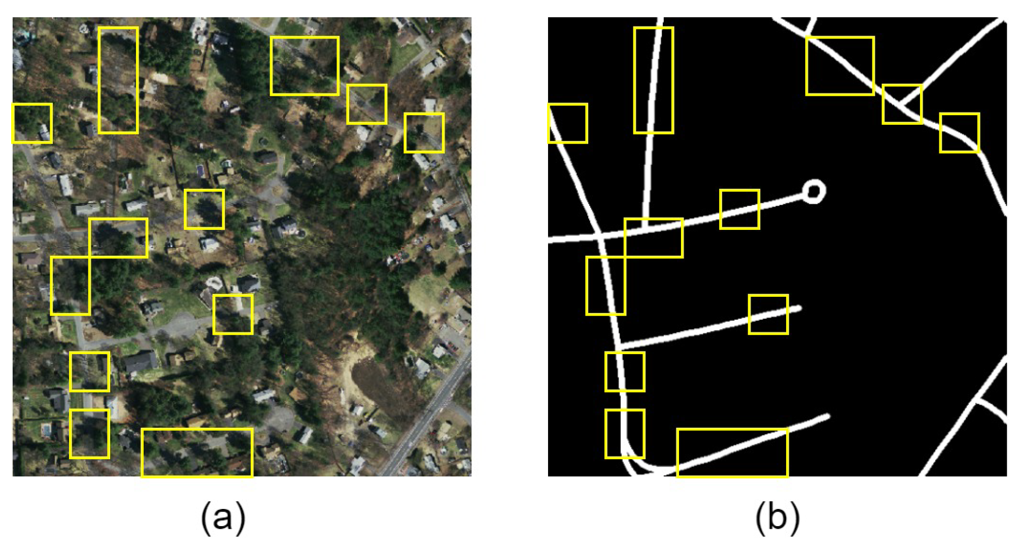
Figure 1. Example of occlusions: (a) RS image; (b) road label. The yellow boxes are occluded areas.
Remotesensing 15 04215 g001
Figure 2. The framework of RemainNet. The backbone of RemainNet adopts transformer blocks. The input of RemainNet is RS image x and mask m. x m is masked features before a transformer block. The features after transformer blocks are f 1 , f 2 , f 3 , and f 4 , respectively. IPM and SPM are convolution modules. IPM and SPM generate image prediction x ^ and semantic prediction y ^ , respectively.
Remotesensing 15 04215 g002
Figure 3. The structure of STB and PM.
Remotesensing 15 04215 g003
Figure 4. The structure of IPM. The input of IPM is features f 1 , f 2 , f 3 , and mask m. The output of IPM is reconstructed image x ^ .
Remotesensing 15 04215 g004
Figure 5. The structure of SPM. The input of IPM is features f 1 , f 2 , f 3 , and f 4 . The output of IPM is road prediction y ^ .
Remotesensing 15 04215 g005
Figure 6. Visual comparisons of different methods on the Massachusetts Roads dataset: (a) remote sensing image, (b) the ground truth, (c) DeepLab v3+, (d) D-LinkNet, (e) NL-LinkNet, (f) MACU-Net, (g) RoadExNet, (h) ours.
Remotesensing 15 04215 g006
Figure 7. Visual comparisons of different methods on the DeepGlobe Road Extraction dataset: (a) remote sensing image, (b) the ground truth, (c) DeepLab v3+, (d) D-LinkNet, (e) NL-LinkNet, (f) MACU-Net, (g) RoadExNet, (h) ours.
Remotesensing 15 04215 g007
Figure 8. Accuracy curves of different thresholds: (a) IoU curves in the Massachusetts Roads dataset, (b) precision–recall in the Massachusetts Roads dataset, (c) IoU curves in the DeepGlobe Road Extraction dataset, (d) precision–recall in the DeepGlobe Road Extraction dataset. curves.
Remotesensing 15 04215 g008
Figure 9. Visual comparisons of original image and reconstructed image; (a) original RS image, (b) unmasked area, (c) reconstructed image, (d) combination of unmasked area and reconstructed image.
Remotesensing 15 04215 g009
Table 2. Road extraction results on the Massachusetts Roads dataset (The bold means highest and lowest value).
MethodPRF1IoU
DeepLab v3+ [27]0.83910.71100.76970.6257
D-LinkNet [49]0.79140.76810.77960.6387
NL-LinkNet [10]0.80450.75810.78060.6402
MACU-Net [38]0.82460.72890.77380.6310
RoadExNet [13]0.80380.75980.78120.6409
RemainNet0.80800.76750.78720.6491
Table 3. Road extraction results on the DeepGlobe Road Extraction dataset (The bold means highest and lowest value).
MethodPRF1IoU
DeepLab v3+ [27]0.78520.75320.76890.6245
D-LinkNet [49]0.73560.78580.75990.6128
NL-LinkNet [10]0.74990.77500.76230.6159
MACU-Net [38]0.78930.71230.74880.5985
RoadExNet [13]0.74310.78090.76160.6149
RemainNet0.76940.79420.78160.6415
Table 4. FLOPs per image and network parameter (The bold means highest and lowest value).
MethodFLOPs/GParameters/M
DeepLab v3+ [27]88.5459.23
D-LinkNet [49]33.5931.10
NL-LinkNet [10]31.4421.82
MACU-Net [38]33.595.15
RoadExNet [13]33.8731.13
RemainNet60.9033.59
Table 5. Ablation study results of IR and SR (The bold means highest and lowest value).
MethodMassachusetts RoadsDeepGlobe Road Extraction
PRF1IoUPRF1IoU
RemainNet without IR and SR0.81260.75410.78220.64230.75380.78730.77020.6263
RemainNet without SR0.80640.76180.78340.64400.75530.79310.77380.6310
RemainNet without IR0.80580.76550.78510.64620.75690.79180.77400.6313
RemainNet0.80800.76750.78720.64910.76940.79420.78160.6415
Table 6. Ablation study results of the mask rate (The highest results are bold in the table).
Mask Rate StrategyMassachusetts RoadsDeepGlobe Road Extraction
PRF1IoUPRF1IoU
keep unchanging(0.75)0.80560.76320.78380.64450.76260.79100.77650.6347
keep unchanging(0.375)0.80150.76770.78420.64500.75310.79970.77570.6336
linearly reduce0.80800.76750.78720.64910.76940.79420.78160.6415
Disclaimer/Publisher’s Note: The statements, opinions and data contained in all publications are solely those of the individual author(s) and contributor(s) and not of MDPI and/or the editor(s). MDPI and/or the editor(s) disclaim responsibility for any injury to people or property resulting from any ideas, methods, instructions or products referred to in the content.