Article

Relationship between CO2 Fertilization Effects, and Stand Age, Stand Type, and Site Conditions

School of Forestry, Northeast Forestry University, Harbin 150040, China
*
Author to whom correspondence should be addressed.
Remote Sens. 2023, 15(17), 4197; https://doi.org/10.3390/rs15174197
Submission received: 23 June 2023 / Revised: 20 August 2023 / Accepted: 22 August 2023 / Published: 26 August 2023

Abstract

:
The CO2 fertilization effect (CFE) plays a crucial role in the amelioration of climate change. Many physiological and environmental factors, such as stand age, stand type, and site conditions, may affect the extent of the CFE. However, the relationship between the CFE and these factors remains elusive. In this study, we used the emerging gross primary production (GPP) remote sensing products, with GPP predicted using eddy covariance–light use efficiency models (EC-LUE GPP) based on satellite near-infrared reflectance of vegetation (NIRv GPP) and assessed with a random forest model to explore the CFE trends with stand age in a coniferous forest and a broad-leaved forest in Heilongjiang Province, China. We additionally compared the differences among the CFEs under different site conditions. The CFEs in coniferous forests and broad-leaved forests both showed a rapid increase in stands of 10 to 20 years of age, followed by a decline after reaching a maximum, with the rate of decline reducing with age. Eventually, CFE remained stable in stands near 100 years of age. However, the CFE in coniferous forests exhibited more extended periods of rapid increase and a higher maximum than in broad-leaved forests. Moreover, in this study, we used the site class index (SCI) to grade site conditions. The results demonstrate that the CFE differed significantly under different levels of site conditions, and these differences gradually decreased with age. The site with the highest SCI had fewer environmental restrictions on the CFE, and consequently, the CFE rate of decline was faster. Our results are of significance in understanding the CFE and adapting to future changes in atmospheric CO2 concentration.

1. Introduction

Since the Industrial Revolution, fossil fuel combustion has increased the atmospheric CO2 concentration from about 280 ppm [1] to 416 ppm in 2020 [2]. The IPCC Sixth Assessment Report indicates that over the past decade, human activities have emitted an average of 10.9 ± 0.9 PgC yr−1 of CO2, of which 31% (3.4 ± 0.9 PgC yr−1) is stored in vegetation in terrestrial ecosystems [3]. The rapidly increasing concentration of CO2 in the atmosphere poses a significant challenge to global sustainable development. Globally, there is particular emphasis on the monitoring of CO2. The rapid development of techniques such as satellite-based estimation of atmospheric CO2 concentrations and monitoring pf CO2 emissions using mobile devices has enabled accurate measurements of CO2 concentrations at various scales. This advancement provides robust support for numerous ecological studies [4,5]. Carbon uptake from terrestrial ecosystems has significantly slowed the rate of climate change. There is considerable evidence that vegetation photosynthesis has gradually increased over the past 60 years, along with the increase in anthropogenic CO2 emissions [6,7], and terrestrial carbon uptake has continued to increase [8,9,10,11]. This phenomenon is due to the increase in vegetation productivity caused by the increase in CO2 concentration [12,13], termed the CO2 fertilization effect (CFE) [14].
CFE varies depending on plant architecture, plant physiology, and environmental factors. [15,16,17,18,19,20]. Therefore, stand age, stand type, and site conditions may have a key impact on CFE. It has been demonstrated that the CFE is higher in juvenile trees and has a stronger effect than in mature and old trees [17,19,21]. However, only the differences between juvenile and old trees have been compared. Thus, a comprehensive evaluation of the relationship between CFE and the overall stand age is lacking. Moreover, thus far, studies have not emphasized the differences between different stand types and site conditions. This has hindered the in-depth understanding of the forest carbon cycle and rational formulation of policies to address climate change.
Existing studies typically utilize traditional methods such as indoor CO2 control experiments, free-air CO2 enrichment (FACE) experiments, flux tower observations, and tree-ring observations [17,22,23,24]. However, these methods have certain drawbacks. Due to space constraints, indoor experiments can only focus on juvenile trees and cannot evaluate mature trees [25,26]. Although FACE solves some of the limitations of indoor experiments [27], the increase in CO2 concentration in the FACE experiment is sudden, which differs from the slow rise in atmospheric CO2 concentration in nature [21]. Therefore, whether the results of FACE experiments can reflect the changes in tree physiology and growth in the natural environment is debatable. Flux tower and tree-ring observation experiments only indicate the level of the sample point, and their spatial continuity is low, in addition to issues with the short time frames during these experiments.
Gross primary production (GPP) denotes the total amount of carbon fixed in the process of photosynthesis by plants in an ecosystem. Quantifying the GPP of terrestrial ecosystems has been an important part of quantifying the global carbon cycle [3]. Moreover, GPP plays an important role in quantifying CFE and investigating the patterns of change in CFE [15]. The carbon cycle process model and remote sensing methods can achieve long-term continuous observation of GPP in a large-scale spatial range, which solves the shortcomings of traditional methods. However, due to the assumptions of the carbon cycle process model, it is difficult to fully parameterize the complex physiological processes of plants, and there can be a great deal of uncertainty in the predicted results [28,29]. Traditional GPP remote sensing products (such as MODIS GPP) also have certain shortcomings, as they do not take into account the direct impact of atmospheric CO2 on light use efficiency (LUE), underestimating the CFE [2]. Recently, some emerging remote sensing GPP products have overcome these shortcomings. Examples are the NIRv GPP dataset, which is estimated by a new type of vegetation index, near-infrared reflectance of vegetation (NIRv) based on remote sensing data [30], and EC-LUE GPP corrected for LUE based on eddy covariance tower flux data [31]. Based on the advantages of these datasets, several studies initially attempted to use multiple regression models to estimate the response of GPP to atmospheric CO2 increases [15,32]. However, compared with traditional regression models, machine learning algorithms (such as the random forest algorithm) are more flexible. They can further integrate the nonlinear influence of each explanatory variable on GPP change and the interaction between variables. Hence, using machine learning algorithms can potentiate the use of these datasets to quantify the response of GPP to changes in the external environment [33].
In this study, we used NIRv GPP and EC-LUE GPP combined with a random forest algorithm to explore the relationship between CFE and stand age, stand type, and site condition in the Heilongjiang region of China from 1982 to 2010. Our objectives were to (a) identify the variation of CFE with stand age, (b) compare the differences in CFE among the different stand types, and (c) compare the differences in CFE among the different site conditions.

2. Dataset

2.1. Study Region

Heilongjiang Province is located in northeast China at 121°11′~135°05′E, 43°26′~ 53°33′N and covers a total area of 4.73 × 10⁷ hm2 (Figure 1). The terrain has a high elevation in the southeast and a low elevation in the southwest and is generally complex. The region belongs to a cold temperate zone and has a temperate continental monsoon climate. The annual average temperature is between −5 and 5 °C, the total annual precipitation is between 400 and 700 mm, and the interannual precipitation variation shows only small fluctuations. The area is rich in vegetation and contains the largest forest areas in China: the Greater Khingan Mountains, the Lesser Khingan Mountains, and the Changbai Mountains forest areas. Coniferous forests dominate the Greater Khingan Mountains [34], while broad-leaved Korean pine forests dominate the Lesser Khingan Mountains [35]. According to statistics from the National Forestry and Grassland Administration of China [36], the forest area of Heilongjiang Province covers 1.99 × 10⁷ hm2, with a forest coverage rate of 43.78% and a forest stock of 1.85 × 10⁹ m3. It has a broad-leaved forest area of 1.37 × 10⁷ hm2, accounting for 68.8% of the province’s forest area. In comparison, the area of coniferous forest is 5.80 × 10⁶ hm2, accounting for 29.2% of the province’s forest area. It is one of the largest forestry provinces in China and plays a vital role in China’s forest carbon uptake and the carbon cycle.

2.2. Study Data

2.2.1. GPP Data

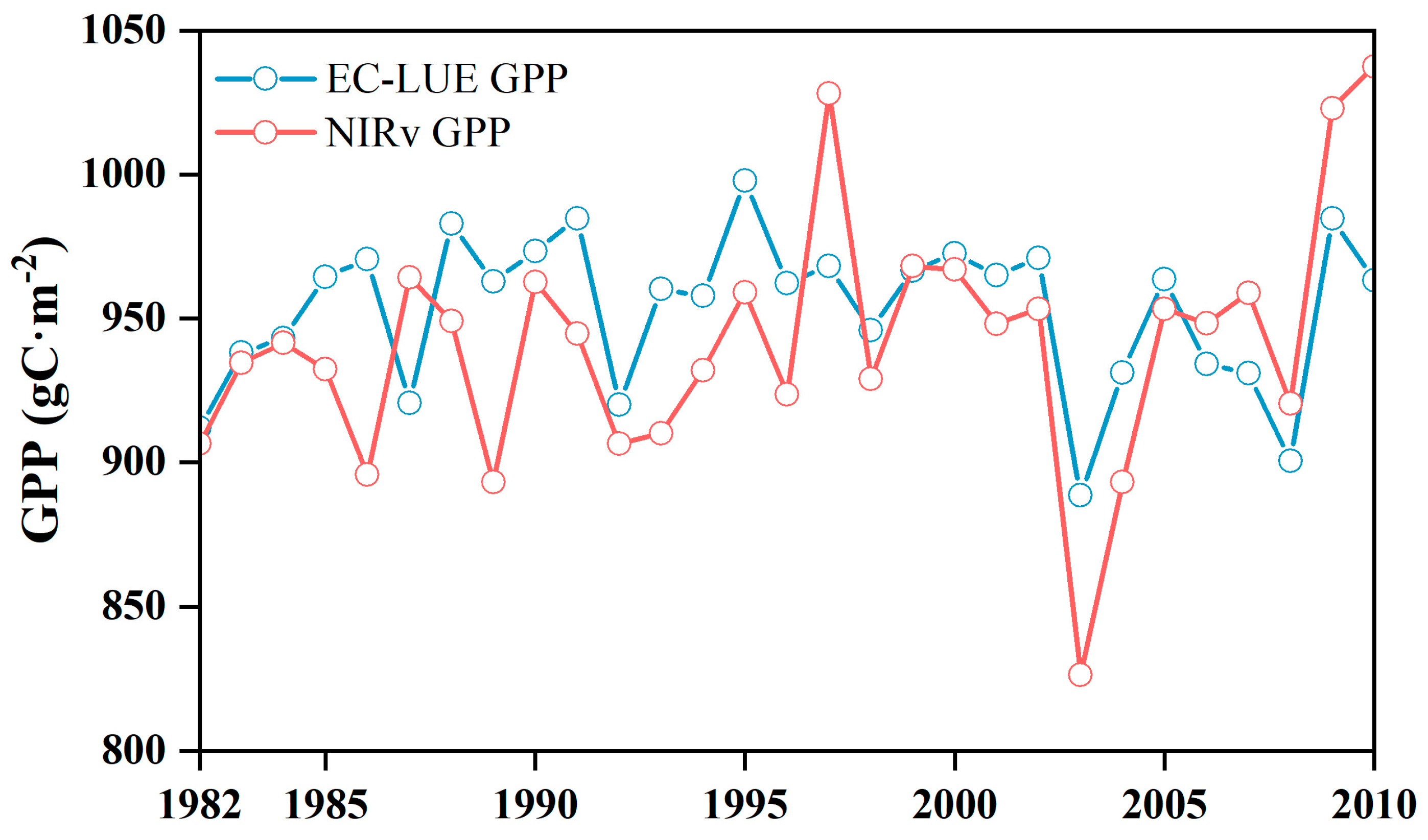
The GPP data used in this study were derived from the global GPP dataset corrected using the EC-LUE model (EC-LUE GPP) [31], and the global GPP dataset was estimated using novel vegetation index NIRv (NIRv GPP) [30]. The EC-LUE GPP data provide global GPP estimates in 8-day intervals from 1982 to 2017 with a spatial resolution of 0.05°. The NIRv GPP data provide global monthly GPP estimates for 1982–2018 with a spatial resolution of 0.05° (Table 1). The changes in annual growth season GPP calculated using ECL-LUE GPP and NIRv GPP were similar and showed no significant trends from 1982 to 2010 (Figure 2).

2.2.2. Environmental and Climatic Data

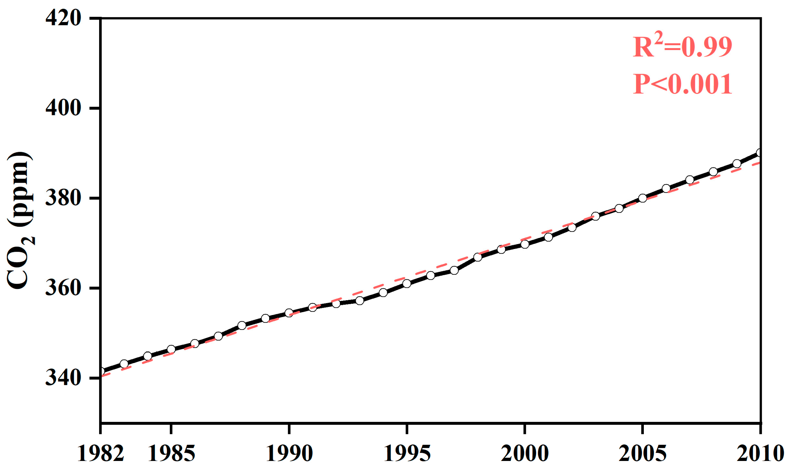
In this study, five environmental factors, namely the annual average atmospheric CO2 concentration (CO2), the growing season (May to September), total nitrogen deposition (Ndep), average temperature (Tmean), total precipitation (Pre), and average water vapor pressure difference (VPD), were selected as growing season total GPP impact factors. The annual mean atmospheric CO2 concentration (CO2) was derived from the annual average atmospheric CO2 concentration data released by the Mauna Loa Observatory in Hawaii, USA, from 1982 to 2010 [37]. The nitrogen deposition (Ndep) data were derived from the historical nitrogen deposition database (1850–2014) in the CCMI nitrogen surface fluxes in support of CMIP6—version 2.0 [38], with a temporal resolution of months and a spatial resolution of 0.5°. The average temperature (Tmean), the total precipitation (Pre), and the average water vapor pressure difference (VPD) were calculated from the CRU TS (version 4.0.5) [39] global meteorological data from 1901 to 2017 provided by the National Centre for Atmospheric Science, with a monthly temporal resolution and a spatial resolution of 0.5° (Table 1). In Heilongjiang Province, China, from 1982 to 2010, the annual average atmospheric CO2 concentration (Figure 3), the growing season total Ndep, Tmean, and average VPD exhibited an increasing trend, whereas the growing season total Pre exhibited a decreasing trend (Figure 4).

2.2.3. Stand Type, Stand Age, and Site Condition

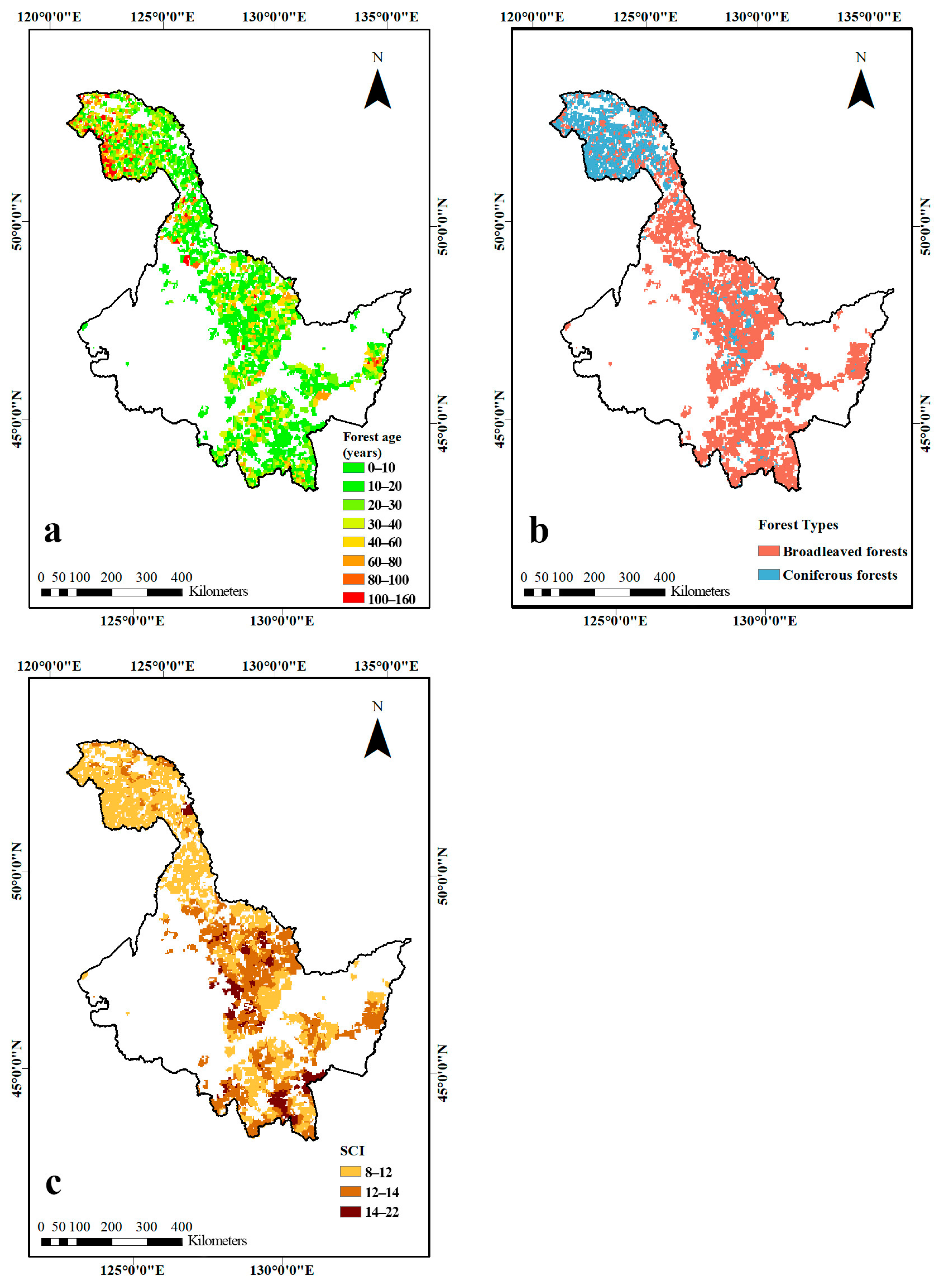
The stand age distribution map in Heilongjiang Province in 1982 (Figure 5a) was based on the data from the eighth national forest inventory from 2009 to 2014 [40]. The per-pixel stand age was interpolated by the Kriging method [41].
The stand type map of Heilongjiang at a 1 km resolution (Figure 5b) was obtained from the Northeast Institute of Geography and Agroecology, Chinese Academy of Sciences, published in 2007. The scale of the map is 1:1,000,000 [42]. It was assumed that the stand type did not change from 1982 to 2010.
We used the site class index (SCI), which relates the relative height of trees of a given age to estimate whether a site is of high, medium, or low quality for tree growth. The SCI distribution map of coniferous and broad-leaved forests in Heilongjiang (Figure 5c) was obtained based on the SCI distribution map of Heilongjiang Province calculated by Wang bin (2018) using forest inventory data [43]. It was assumed that the quality of sites, as estimated by the SCI, did not change from 1982 to 2010.

3. Methods

3.1. Variable Selection and Importance Analysis

In this study, EC-LUE GPP and NIRv GPP during the annual growing season were used as the observation variables. The annual average CO2 concentration, growing season (May to September), total nitrogen deposition (Ndep), average temperature (Tmean), total precipitation in the growth season (Pre), and average water vapor pressure difference (VPD) were used as the impact factors. The VPD was calculated according to Equations (1) and (2).
V P D = S V P V A P
S V P = 0.6107 × e 17.38 T m e a n / ( 239.0 + T m e a n )
where SVP is the saturated vapor pressure, VAP is the actual vapor pressure, and Tmean (°C) is the average annual temperature.
In this study, the Boruta [44] feature selection method was employed to rank and filter the five extracted variables. Boruta is a random-forest-based screening approach. It iteratively removes the features that are proven by a statistical test to be less relevant than random probes [44]. This method ultimately categorizes the variables into confirmed variables and rejected variables. In the variable importance analysis, we employed %IncMSE as a metric to measure variable importance, and after numerical changes, the sum was 100. A high %IncMSE value of a variable indicates its importance for model prediction.

3.2. Calculation of GPP Responses to Atmospheric CO2 Concentrations

The GPP datasets used in this study were preprocessed. All data were resampled to a resolution of 1 × 1 km, and all data were spatially referenced. To accentuate the differences, we quantified CFE using the approximate formula of β = G P P C O 2 proposed by Keeling in 1973 [14] Equation (3), represents the change in GPP for every 100 ppm increase in atmospheric CO2 concentration. The response of GPP to changes in atmospheric CO2 concentrations ( β G P P ) was estimated using EC-LUE GPP and NIRv GPP combined with a random forest model and by setting two scenario modes to control CO2 change. Scenario 1 (S1): All climate and atmospheric variables change realistically over time. Scenario 2 (S2): Atmospheric CO2 concentrations were kept unchanged at 1982 levels, with other climate and atmospheric variables changing realistically over time. The difference between the GPP estimates in these two scenarios (∆GPP) is the extent of change in GPP caused by atmospheric CO2 concentrations.
β G P P = G P P C O 2 × 100
where β G P P represents the change in GPP for every 100 ppm increase in atmospheric CO2 concentration, ΔGPP represents the amount of change in GPP caused by CO2 changes, and ΔCO2 represents the amount of change in CO2.
We trained the random forest model for scenario 1, and the GPP on each pixel in the study area under scenario 2 was reconstructed through the model. For example, the 1983 GPP was rebuilt, as shown in Equations (4) and (5).
S 1 : G P P 1983 ~ ( C O 2 1983 , T m e a n 1983 , P r e 1983 , V P D 1983 , N d e p 1983 )
S 2 : G P P 1983 ~ ( C O 2 1982 , T m e a n 1983 , P r e 1983 , V P D 1983 , N d e p 1983 )
In the estimation process, we selected 28 years from 1982 to 2010 to train the model and the remaining 1 year for cross validation of the model (29 years in total). The model was run a total of 28 times to ensure that the simulated values were tested for each year from 1982 to 2010, and the final GPP values of the model simulation were the average of the 28 results. Finally, we calculated the β G P P of each pixel on a per-year basis using the ∆GPP of each pixel and its corresponding ΔCO2 from 1982 to 2010 (Equation (6)).
β G P P t = G P P S 1 t G P P S 2 t C O 2 t C O 2 1982 × 100
where t represents the year of calculation; β G P P t represents the response of GPP to atmospheric CO2 concentrations in t; G P P S 1 t and G P P S 2 t represent the predicted values of GPP under the S1 and S2 scenarios in t, respectively; C O 2 t represents the global average CO2 concentration in t; and C O 2 1982 represents the global average CO2 concentration in 1982.

3.3. Analysis of the Variation of β G P P with Stand Age

We used coniferous forests (CFs) and broad-leaved forests (BFs) with a stand age of 1–100 years as research objects. We matched the annual β G P P of all pixels with stand age, and we considered the average β G P P at the same stand age to be the final estimate of the β G P P for that stand age (Equation (7)). Finally, we use nonlinear regression to assess the relationship between β G P P and stand age (Equation (8)). We observed that the relationship between β G P P and stand age was similar among the different remote sensing products used within the same stand type. As a result, in order to more clearly compare the differences between different stand types, we utilized the average of the β G P P derived from these two remote sensing datasets to construct the relationship between β G P P and stand age for each stand type.
β y L = i = 1 n β i y L n
β G P P = a 1 + b a g e c d 1 e a g e c
where in Equation (7), β y L represents the CFE when the stand age is y under L stand type, β i y L represents the CFE intensity of the ith pixel (i = 1…n) under L stand type when the stand age is y, n represents the number of pixels corresponding to y stand age. In Equation (8), β G P P represents the change in GPP for every 100 ppm increase in atmospheric CO2 concentration; and a, b, c, and d are nonlinear regression model parameters, where parameter a determines the general magnitude of β G P P , and b, c, and d are parameters determining the rate of β G P P changing with stand age. The maximum value of β G P P increases with the increase in parameters b and d, the stand age at which the maximum value is reached increases with the increase in parameters c and d.

3.4. Comparison of the Differences in β G P P among Different Conditions

We divided the site conditions into three levels based on SCI values in order to ensure a balanced number of pixels for different site levels. Therefore, an SCI value lower than 12 corresponds to the “low-quality” site condition, a between 12 and 14 corresponds to the “medium-quality” site condition, and a value greater than 14 corresponds to the “high-quality” site condition. In contrast to exploring the impact of stand age on the CO2 fertilization effect, when exploring the influence of site conditions on the CO2 fertilization effect, greater emphasis should be placed on long-term effects; therefore, we employed a β calculation approach distinct from that used to explore the effects of forest age. We calculated the annual ∆GPP of each pixel at different site levels from 1982 to 2010, as well as its corresponding ΔCO2, and performed a linear regression analysis (Equation (9)). The slope of the obtained regression model represents the overall β G P P of each pixel from 1982 to 2010 ( β 1982 2010 ). To obtain a more accurate estimate under varying site conditions, we utilized the two different remote sensing products and calculated the average of β G P P to represent the CFE of each pixel. To reduce the effect of stand age, we formed groups covering 20-year intervals based on stand age in 1982 and used the average β G P P of all pixels in the same age group as the final estimate.
G P P = β 1982 2010 100 C O 2 + ε
where ∆GPP represents the difference between GPP values at S1 and S2 ,   β 1982 2010 represents the change in GPP for every 100 ppm increase in atmospheric CO2 concentration from 1982 to 2010, C O 2 represents the difference between the annual global CO2 average and the 1982 global CO2 average, and ε is the residual error term.

4. Results

4.1. Random Forest Model Validation

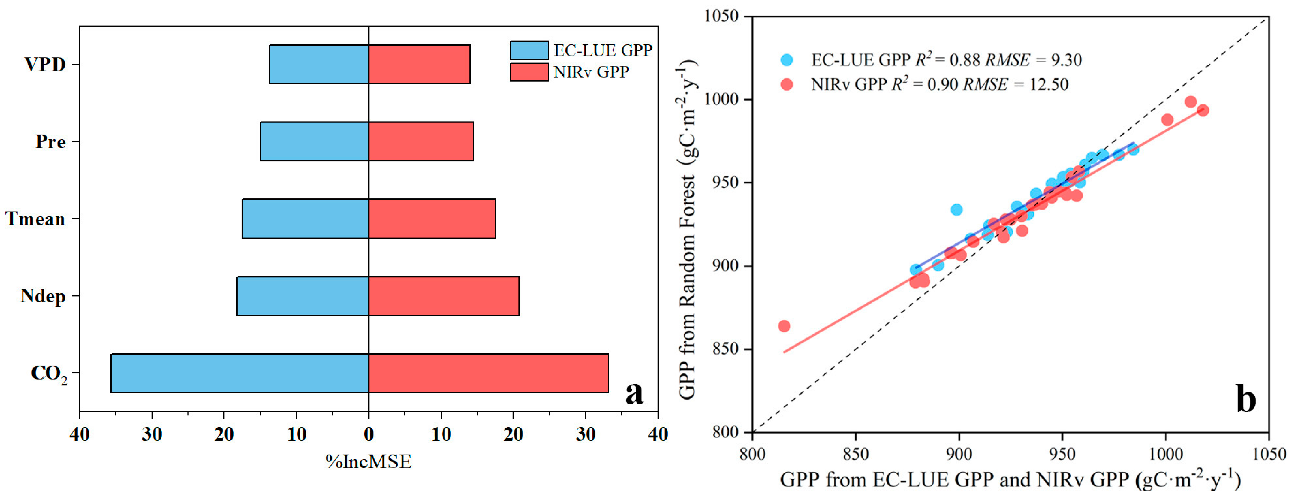
The Boruta feature selection results show that the five variables of CO2, Ndep, Tmean, Pre, and VPD were all confirmed. The variable importance rankings of the two remote sensing datasets (EC-LUE GPP and NIRv GPP) are identical, with CO2, Ndep, Tmean, Pre, and VPD ranked in descending order of importance (Figure 6a). The random forest model trained by two remote sensing datasets (EC-LUE GPP and NIRv GPP) performed well in validation, with coefficients of determination (R2) of 0.88 and 0.90, respectively, and RMSE values of 9.30 and 12.50, respectively (Figure 6b). Therefore, the random forest model was reliable for use in the GPP simulation.

4.2. Variation of the CO2 Fertilization Effect (CFE) with Stand Age

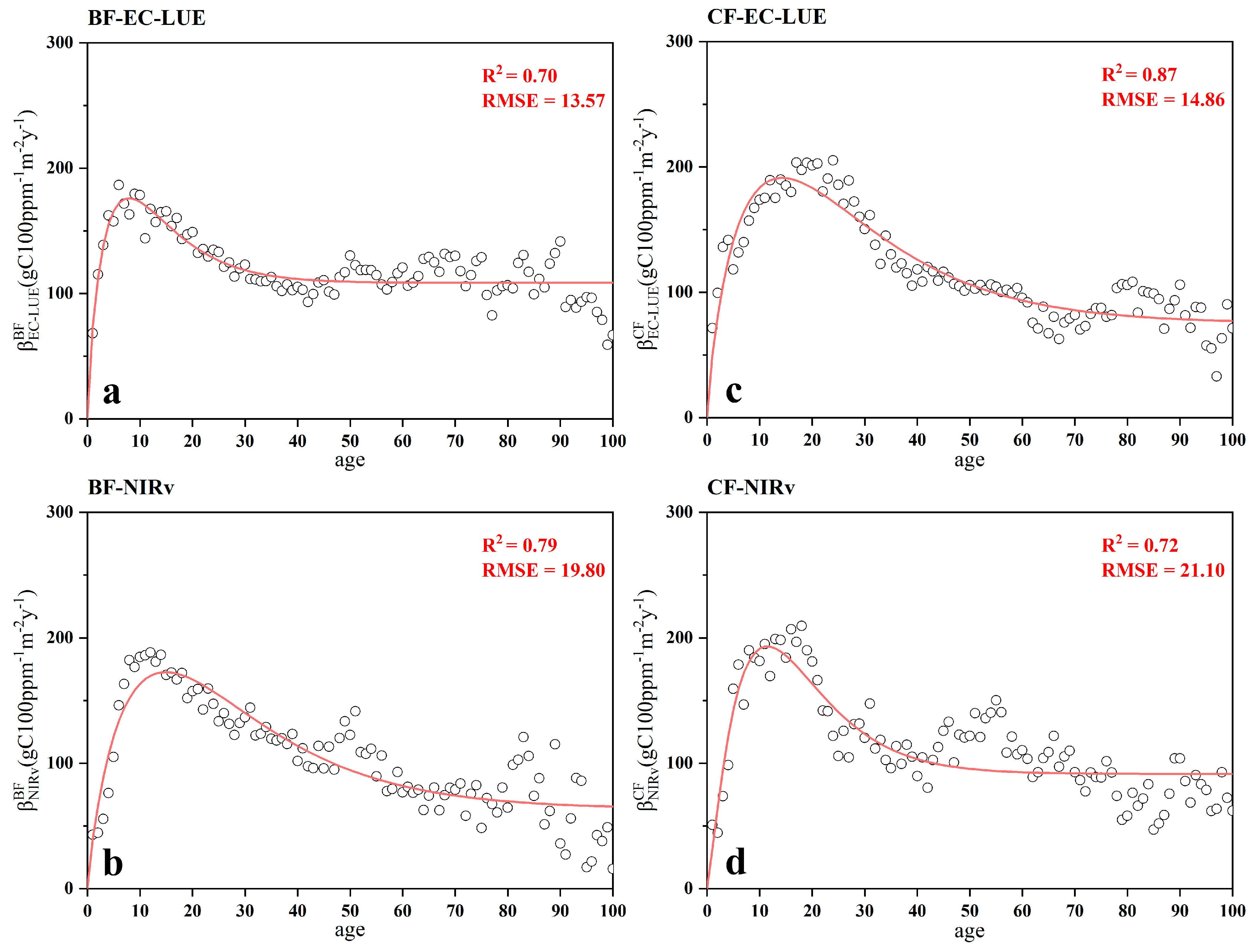
Both remote sensing data types showed that in coniferous forests and broadleaf forests of 100 years of age, β G P P initially exhibited a trend of rapid increase with age, whereas after reaching a maximum, β G P P declined. During the declining period, the rate of decline gradually decreased until β G P P ultimately stabilized. (Figure 7). In both forest types, the maximum values of β G P P occurred in younger stands for the broad-leaved forests at around 10 years of age ( β E C L U E m a x B F = 179.44, age = 9; β N I R v m a x B F = 188.52, age = 12) and for coniferous forests at around 20 years of age ( β E C L U E m a x C F = 203.46, age = 19; β N I R v m a x C F   = 209.75, age = 18), and the minimum values occurred in older stands ( β E C L U E m i n B F = 59.10, age = 99; β N I R v m i n B F = 15.79, age = 100; β E C L U E m i n C F = 32.97, age = 97; β N I R v m i n C F = 47.09, age = 86). The regression coefficients for the different remote sensing products and stand types are presented in Table 2. The R2 and the RMSE indicate that the nonlinear regression model we used could fit well the relationship between β G P P and stand age.

4.3. Differences in CFE between Different Stand Types

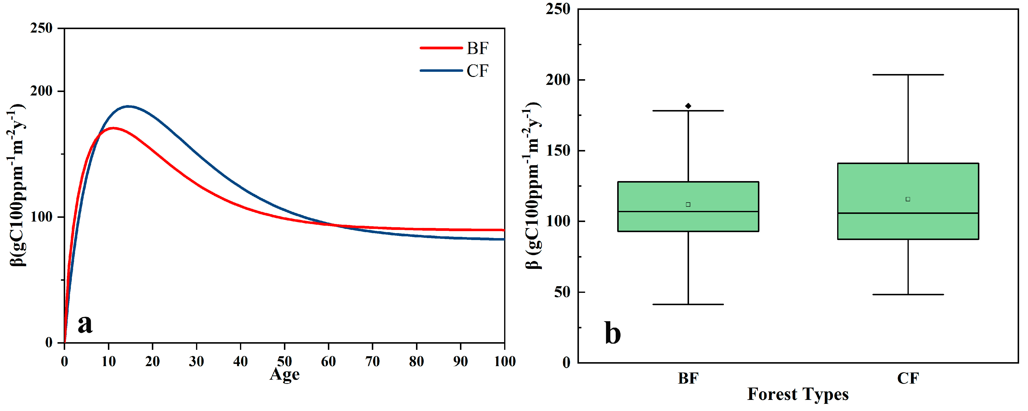
In both forest types, the average value of the β G P P calculated by the two remote sensing products also showed a trend of first increasing, then decreasing and eventually stabilizing with age (Figure 8a). In broad-leaved forests and coniferous forests, the highest average β G P P occurred at 10 ( β m a x B F = 181.60) and 18 ( β m a x C F = 203.64) years of stand age, respectively, whereas the minimum appeared at 100 ( β m i n B F = 41.29) and 97 ( β m a x C F = 48.26) years of stand age, respectively. Comparing the nonlinear regression results between the two stand types, the β G P P of coniferous forests had a longer increasing phase, and the maximum value was higher than that of broad-leaved forests (Figure 8a). The β G P P of the two stand types began to decline at a stand age of 11 and 16 years, respectively. The β G P P of both stand types reached the same level at about 60 years of stand age. Finally, the β G P P of broad-leaved forests was stable around 89.70 gC100 ppm−1m−2y−1, and the coniferous forest β G P P was stable around 82.00 gC100 ppm−1m−2y−1. Overall, there was no significant difference in the β G P P between the coniferous forest and broad-leaved forest in the age range of 1–100 years (p = 0.45, β ¯ G P P C F = 115.57, β ¯ G P P B F = 111.78) (Figure 8b).

4.4. Differences in CFE among Different Site Conditions

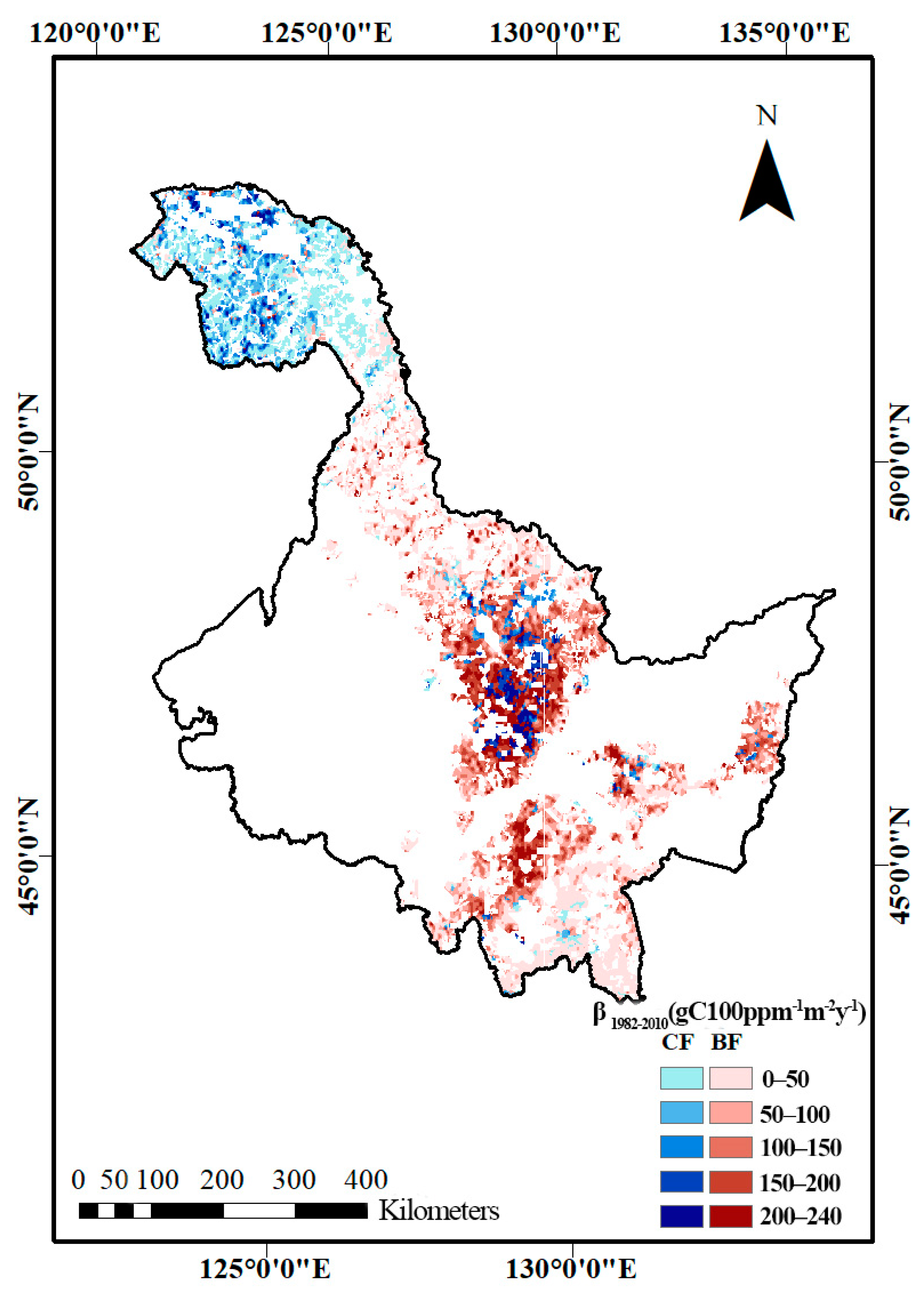
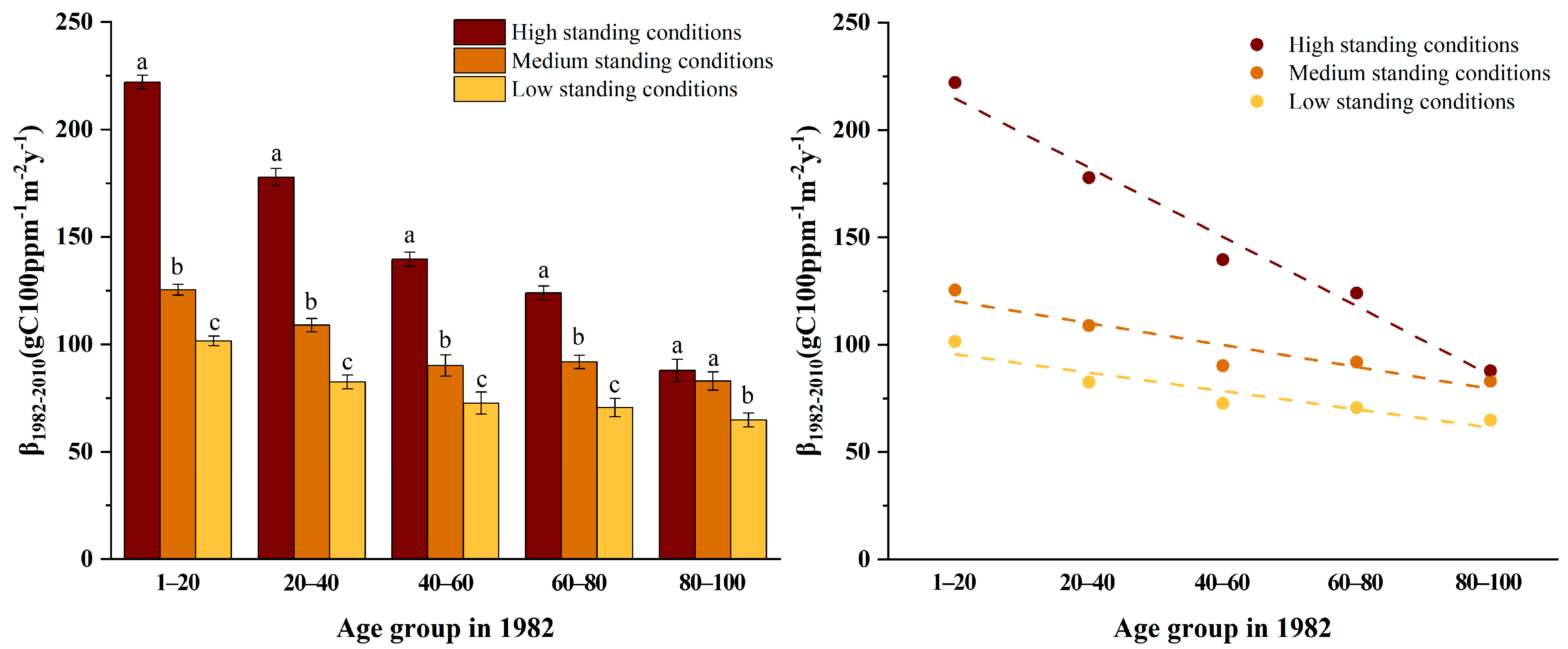
The spatial distribution of CFE in the study region is illustrated in Figure 9. When combined with the spatial distribution of site conditions (Figure 5c), we found that across all stand age groups, the CFE was the highest under high-quality site conditions, followed by medium-quality site conditions and low-quality site conditions. In young trees, the CFE in high-quality sites was much higher than that in medium- and low-quality sites (Figure 10). As the trees matured, a 60% decline in CFE occurred at high-quality sites compared to a 35% decline at the medium- and low-quality sites, such that the CFE at high-quality sites in 80–100-year-old trees was not significantly different from that at medium-quality sites and only slightly higher than that at low-quality sites (Figure 10).

5. Discussion

Our study found that in Heilongjiang, China, both broad-leaved and coniferous forests exhibited substantial differences in CFE depending on the age of the trees and the quality of the site. Initially, there was a rapid increase in the CFE in young trees, reaching a maximum between 10 and 20 years, with a gradual decline until the stand age reached 100 years, at which point the CFE tended to stabilize. These results indicate that the ability of the same forests to offset elevated CO2 in the atmosphere at different growth stages is not consistent, and this ability has a significant nonlinear relationship with stand age. Moreover, we found that the CFE differed across stand types. Compared to broad-leaved forests, the CFE in coniferous forests had a longer period of rapid increase and a higher maximum value. We also found that the quality of the site was critically important, with young trees at high-quality sites having CFE values more than twice those at low-quality sites. However, in more mature stands (80–100 years old) the CFE values of high-quality sites were much lower—only slightly higher than those of low-quality sites. In our study, we used different GPP data products to estimate CFE, and we found that the results of different products were relatively consistent, enhancing the authenticity of the reported results.
Several factors have been suggested to enhance the CFE. (a) Higher CO2 concentrations in the external environment directly increase the CO2 content and the ratio of CO2 to O2 in green vegetation leaves, which stimulates carboxylation by the Rubisco enzyme in the leaves to increase the photosynthetic rate of the vegetation [19]. (b) Increased CO2 concentration reduces the degree of stomatal opening in leaves, improves water use efficiency in vegetation, and stimulates GPP [45]. (c) Increasing the CO2 concentration may promote an increase in leaf area index (LAI), corresponding to a larger light interception area, thereby increasing the photosynthesis output [46,47].
The juvenile stage of trees is a critical period for their growth and development. When the carbon storage capacity of trees is low, rapid material accumulation is required, and the cells in the leaves have a strong metabolism and strong photosynthesis potential [48]. Increasing the atmospheric CO2 concentration can help to promote tree photosynthesis, increase nutrient and water absorption and utilization efficiency [21], and promote their growth and development. Therefore, vegetation has a higher demand for CO2 and a higher CFE during the juvenile stand stage. The LAI is also relatively low in a juvenile tree stand. With the increase in stand age, the amount of vegetation increases, and the LAI increases rapidly [49], which may be an important reason for the rapid increase in CFE. As the age increases, the forest’s carbon absorption and turnover gradually reach equilibrium [17]. Several studies have shown that trees are subjected to more severe nutrient and water restrictions as they age [22,40,41,42,43,44,45,46,47,48,49,50,51,52], and this restriction may become more severe as the atmospheric CO2 concentration increases [53,54,55]. This limiting effect further inhibits CFE, so the intensity of CO2 fertilization begins to decline as the tree age increases. The adaptation of trees to gradually increasing atmospheric CO2 concentrations may also be an important factor affecting the reduced impact of the CFE [56]. Our findings are consistent with observations using radial growth of trees, such as those of Geoff Wang et al. [21], that the CFE in juvenile trees is higher than that in old trees. However, some studies suggest that CFE is absent during the tree aging stage [19,57]. They suggest that due to environmental and physiological limitations of the older trees in their study area, the CO2 concentration exceeded the maximum carbon absorption capacity of stands with older-aged trees [58,59], so they will not react to a further increase in CO2 concentration. Most of these studies focus on observing tree rings, which differ from the GPP levels we observed. Some studies have also found that the biomass distribution is different in older trees compared to younger trees, characterized by the transfer of excess carbon to the roots and the soil and reduced carbon transfer to the stem, resulting in the inability to reflect the fertilization effect of atmospheric CO2 in tree rings [60,61,62]. Therefore, unlike our studies, studies on tree rings are not able to detect the effects of CFE on the GPP of older trees.
In terms of the differences in the CFE among different stand types, our study found that coniferous forests had a lengthier stage of β G P P increase compared to broad-leaved forests. We believe this is mainly due to different growth strategies and physiological adaptations among different stand types. Broad-leaved forests usually grow rapidly during the juvenile tree stage, but with the increase in tree age, the growth rate gradually slows down, entering the mature stage relatively early. Their responses to changes in the external environment are more pronounced. In contrast, juvenile coniferous forests grow relatively slowly, and their growth periods can last longer. We also found that the CFE in coniferous forests had a higher maximum value than in broad-leaved forests. This is because evergreen coniferous forests typically occupy poorer-quality habitats than deciduous broad-leaved forests and have higher nutrient uptake and water efficiency [63,64,65,66]. The leaf N and P content of broad-leaved trees is higher, while the C content is lower than that of coniferous trees [65,67]. Therefore, under similar N and P nutrient conditions, the leaf formation efficiency of evergreen coniferous forests is significantly higher than that of deciduous broad-leaved forests [68,69]. As a result, coniferous forests have a higher photosynthetic potential under similar environmental conditions.
SCI is a comprehensive evaluation of forest site conditions. Many studies have shown that a forest’s growth status and productivity are closely related to site conditions [43,70]. We found that the CFE under high-quality site conditions was significantly higher than that under medium- and low-quality site conditions, consistent with previous research findings on nutrient and water constraints [20,21,22,52]. These studies suggest that areas poor nutrient and water conditions, such as low soil P and N content and arid environments, strongly limit CFE. In contrast, the limiting effect is weak or non-existent in areas with good nutrient and water conditions. A more suitable climate and terrain under high-quality site conditions can indirectly enhance the CFE. Our research also found that the age constraints are more pronounced due to the lower environmental constraints under high-quality site conditions, so the CFE in high-quality sites decreases faster with age. In addition, our results indicate that at the juvenile forest stage (1–20 years of age), the differences in CFE among different site quality levels were the greatest, and the environmental constraints were the strongest. This is due to the strong photosynthetic capacity of juvenile trees and their high demand for water, nutrition, and other inputs. As a result, site conditions significantly impact CO2 fertilization. With increased stand age, the difference across site levels gradually narrows, and the difference between high-quality and medium-quality site conditions disappears at the aging forest stage (80–100 years of age). We suggest that this is mainly due to the low photosynthetic potential of aging forests and the small margin for further increase in photosynthesis. As a result, high-quality site conditions cannot promote the further enhancement of CFE.
We used remote sensing to obtain results at large spatial scales. This approach can also provide a solution to the problems of human interference and spatial discontinuity in traditional methods. Compared to research on smaller areas and individual trees, we can more fully evaluate the impact of various complex factors on forest ecosystems, which is more consistent with the natural conditions and the interactions between different factors. However, our research is subject to some shortcomings. First, in estimating the relationship between CFE and stand age, we cannot completely exclude the interference of factors other than stand age. However, the different stand ages were evenly distributed on spatial and temporal scales so that the extent of interference of other factors under different stand ages was similar. Therefore, we believe that such interference would not have a large impact on the overall trend. Secondly, the focus of this study was GPP, which can only reflect the early responses of vegetation to CO2 increase. In the next step, we will explore the responses of NPP and NEP levels to CO2 increase to more comprehensively evaluate the effects of CO2 fertilization. Finally, the physiological adaptations of the vegetation to the gradual increase in atmospheric CO2 concentration are unclear, so the trend of CFE changes with stand age at different times and across different stand types and site conditions may not be consistent. In the next steps, we will further eliminate other interference factors to achieve a more complete and more accurate exploration of CFE and its trend to improve our understanding of the impact of CFE to aid the management of climate change effects.

6. Conclusions

We used emerging remote sensing products to explore the relationship between CFE and stand age changes and compared the changes in CFE among different stand types and site conditions. Our study found that: (a) In both coniferous forests and broadleaf forests, with age, CFE exhibits a trend of an initial rapid increase to a maximum followed by a decline. During the decline period, the rate of decline gradually decreases until CFE stabilizes. (b) Between the two forest types, CFE in coniferous forests had a more prolonged period of rapid increase and a higher maximum. (c) The CFE was significantly higher under high-quality site conditions than under medium- and low-quality site conditions at all stand ages, except 80–100 year group, where no significant difference was observed between high-quality site conditions and medium-quality site conditions. Medium-quality site conditions exhibited a significantly higher CFE than low-quality site conditions across all age groups. Moreover, the differences between the different site quality levels gradually decreased with the forest age. The above results indicate that the CFE has a significant nonlinear relationship with stand age, and high-quality site conditions can further enhance the CFE. These results provide insights to explore the factors impacting the CFE and provide theoretical support for the formulation of future carbon neutrality policies.

Author Contributions

Conceptualization, methodology, writing—original draft, formal analysis, investigation, and visualization, S.B.; conceptualization, validation, resources, writing—review and editing, supervision, and project administration, B.W.; conceptualization, resources, supervision, and project administration, M.L.; formal analysis and investigation, X.K.; formal analysis, J.S.; investigation, Y.C.; resources and supervision, W.F. All authors have read and agreed to the published version of the manuscript.

Funding

This research was funded by the National Key Research and Development Program of China (2020YFC1511603-1), the Fundamental Research Funds for the Central Universities (2572022DT03), and Carbon neutrality special scientific Foundation project HFW220100054.

Data Availability Statement

Data will be made available on request.

Conflicts of Interest

The authors declare no conflict of interest.

References

  1. Etheridge, D.M.; Steele, L.P.; Langenfelds, R.L.; Francey, R.J.; Barnola, J.-M.; Morgan, V.I. Natural and anthropogenic changes in atmospheric CO2over the last 1000 years from air in Antarctic ice and firn. J. Geophys. Res. Atmos. 1996, 101, 4115–4128. [Google Scholar] [CrossRef]
  2. Keenan, T.F.; Luo, X.; De Kauwe, M.G.; Medlyn, B.E.; Prentice, I.C.; Stocker, B.D.; Smith, N.G.; Terrer, C.; Wang, H.; Zhang, Y.; et al. RETRACTED ARTICLE: A constraint on historic growth in global photosynthesis due to increasing CO2. Nature 2021, 600, 253–258. [Google Scholar] [CrossRef] [PubMed]
  3. Canadell, J.G.; Monteiro, P.M.S.; Costa, M.H.; Cotrim da Cunha, L.; Cox, P.M.; Eliseev, A.V.; Henson, S.; Ishii, M.; Jaccard, S.; Koven, C.; et al. Global Carbon and other Biogeochemical Cycles and Feedbacks. In Climate Change 2021: The Physical Science Basis. Contribution of Working Group I to the Sixth Assessment Report of the Intergovernmental Panel on Climate Change; Masson-Delmotte, V., Zhai, P., Pirani, A., Connors, S.L., Péan, C., Berger, S., Caud, N., Chen, Y., Goldfarb, L., Gomis, M.I., et al., Eds.; Cambridge University Press: Cambridge, UK; New York, NY, USA, 2021; pp. 923–1054. [Google Scholar] [CrossRef]
  4. Pei, Z.; Han, G.; Shi, T.; Ma, X.; Gong, W. A XCO Retrieval Algorithm Coupled Spatial Correlation for the Aerosol and Carbon Detection Lidar. Atmos. Environ. 2023, 309, 119933. [Google Scholar] [CrossRef]
  5. Shi, T.; Han, G.; Ma, X.; Mao, H.; Chen, C.; Han, Z.; Pei, Z.; Zhang, H.; Li, S.; Gong, W. Quantifying factory-scale CO2/CH4 emission based on mobile measurements and EMISSION-PARTITION model: Cases in China. Environ. Res. Lett. 2023, 18, 034028. [Google Scholar] [CrossRef]
  6. Zhu, Z.; Piao, S.; Myneni, R.B.; Huang, M.; Zeng, Z.; Canadell, J.G.; Ciais, P.; Sitch, S.; Friedlingstein, P.; Arneth, A.; et al. Greening of the Earth and its drivers. Nat. Clim. Chang. 2016, 6, 791–795. [Google Scholar] [CrossRef]
  7. Mao, J.; Ribes, A.; Yan, B.; Shi, X.; Thornton, P.E.; Séférian, R.; Ciais, P.; Myneni, R.B.; Douville, H.; Piao, S.; et al. Human-induced greening of the northern extratropical land surface. Nat. Clim. Chang. 2016, 6, 959–963. [Google Scholar] [CrossRef]
  8. Sarmiento, J.L.; Gloor, M.; Gruber, N.; Beaulieu, C.; Jacobson, A.R.; Fletcher, S.E.M.; Pacala, S.; Rodgers, K. Trends and regional distributions of land and ocean carbon sinks. Biogeosciences 2010, 7, 2351–2367. [Google Scholar] [CrossRef]
  9. Ballantyne, A.; Smith, W.; Anderegg, W.; Kauppi, P.; Sarmiento, J.; Tans, P.; Shevliakova, E.; Pan, Y.; Poulter, B.; Anav, A.; et al. Accelerating net terrestrial carbon uptake during the warming hiatus due to reduced respiration. Nat. Clim. Chang. 2017, 7, 148–152. [Google Scholar] [CrossRef]
  10. Friedlingstein, P.; O’Sullivan, M.; Jones, M.W.; Andrew, R.M.; Hauck, J.; Olsen, A.; Peters, G.P.; Peters, W.; Pongratz, J.; Sitch, S.; et al. Global Carbon Budget 2020. Earth Syst. Sci. Data 2020, 12, 3269–3340. [Google Scholar] [CrossRef]
  11. Walker, A.P.; De Kauwe, M.G.; Bastos, A.; Belmecheri, S.; Georgiou, K.; Keeling, R.F.; McMahon, S.M.; Medlyn, B.E.; Moore, D.J.P.; Norby, R.J.; et al. Integrating the evidence for a terrestrial carbon sink caused by increasing atmospheric CO2. New Phytol. 2021, 229, 2413–2445. [Google Scholar] [CrossRef]
  12. Beedlow, P.A.; Tingey, D.T.; Phillips, D.L.; Hogsett, W.E.; Olszyk, D.M. Rising Atmospheric CO2 and Carbon Sequestration in Forests. Front. Ecol. Environ. 2004, 2, 315–322. [Google Scholar] [CrossRef]
  13. Huntzinger, D.N.; Michalak, A.M.; Schwalm, C.; Ciais, P.; King, A.W.; Fang, Y.; Schaefer, K.; Wei, Y.; Cook, R.B.; Fisher, J.B.; et al. Uncertainty in the response of terrestrial carbon sink to environmental drivers undermines carbon-climate feedback predictions. Sci. Rep. 2017, 7, 4765. [Google Scholar] [CrossRef] [PubMed]
  14. Ekdahl, C.A.; Keeling, C.K. Atmospheric carbon dioxide and radiocarbon in the natural carbon cycle: I. Quantitative deductions from records at Mauna Loa Observatory and at the South Pole. Brookhaven Symp. Biol. 1973, 24, 51–85. [Google Scholar]
  15. Wang, S.; Zhang, Y.; Ju, W.; Chen, J.M.; Ciais, P.; Cescatti, A.; Sardans, J.; Janssens, I.A.; Wu, M.; Berry, J.A.; et al. Recent global decline of CO2 fertilization effects on vegetation photosynthesis. Science 2020, 370, 1295–1300. [Google Scholar] [CrossRef] [PubMed]
  16. Adams, M.A.; Buckley, T.N.; Turnbull, T.L. Diminishing CO2-driven gains in water-use efficiency of global forests. Nat. Clim. Chang. 2020, 10, 466–471. [Google Scholar] [CrossRef]
  17. Jiang, M.; Medlyn, B.E.; Drake, J.E.; Duursma, R.A.; Anderson, I.C.; Barton, C.V.M.; Boer, M.M.; Carrillo, Y.; Castañeda-Gómez, L.; Collins, L.; et al. The fate of carbon in a mature forest under carbon dioxide enrichment. Nature 2020, 580, 227–231. [Google Scholar] [CrossRef]
  18. Ciríaco da Silva, E.; Nogueira, R.J.; Silva, M.; Albuquerque, M. Drought Stress and Plant Nutrition. Plant Stress 2010, 5, 32–41. [Google Scholar]
  19. Hararuk, O.; Campbell, E.M.; Antos, J.A.; Parish, R. Tree rings provide no evidence of a CO2 fertilization effect in old-growth subalpine forests of western Canada. Glob. Change Biol. 2019, 25, 1222–1234. [Google Scholar] [CrossRef]
  20. Reich, P.B.; Hobbie, S.E.; Lee, T.; Ellsworth, D.S.; West, J.B.; Tilman, D.; Knops, J.M.H.; Naeem, S.; Trost, J. Nitrogen limitation constrains sustainability of ecosystem response to CO2. Nature 2006, 440, 922–925. [Google Scholar] [CrossRef]
  21. Wang, G.G.; Chhin, S.; Bauerle, W.L. Effect of natural atmospheric CO2 fertilization suggested by open-grown white spruce in a dry environment. Glob. Change Biol. 2006, 12, 601–610. [Google Scholar] [CrossRef]
  22. Ellsworth, D.S.; Anderson, I.C.; Crous, K.Y.; Cooke, J.; Drake, J.E.; Gherlenda, A.N.; Gimeno, T.E.; Macdonald, C.A.; Medlyn, B.E.; Powell, J.R.; et al. Elevated CO2 does not increase eucalypt forest productivity on a low-phosphorus soil. Nat. Clim. Change 2017, 7, 279–282. [Google Scholar] [CrossRef]
  23. Fernández-Martínez, M.; Vicca, S.; Janssens, I.A.; Ciais, P.; Obersteiner, M.; Bartrons, M.; Sardans, J.; Verger, A.; Canadell, J.G.; Chevallier, F.; et al. Atmospheric deposition, CO2, and change in the land carbon sink. Sci. Rep. 2017, 7, 9632. [Google Scholar] [CrossRef] [PubMed]
  24. Ainsworth, E.A.; Long, S.P. What have we learned from 15 years of free-air CO2 enrichment (FACE)? A meta-analytic review of the responses of photosynthesis, canopy properties and plant production to rising CO2. New Phytol. 2005, 165, 351–372. [Google Scholar] [CrossRef] [PubMed]
  25. Johnson, D.W.; Ball, J.T.; Walker, R.F. Effects of CO2 and nitrogen fertilization on vegetation and soil nutrient content in juvenile ponderosa pine. Plant Soil 1997, 190, 29–40. [Google Scholar] [CrossRef]
  26. Winter, K.; Aranda, J.; Garcia, M.; Virgo, A.; Paton, S.R. Effect of elevated CO2 and soil fertilization on whole-plant growth and water use in seedlings of a tropical pioneer tree, Ficus insipida Willd. Flora 2001, 196, 458–464. [Google Scholar] [CrossRef]
  27. Allen, L.H.; Drake, B.G.; Rogers, H.H.; Shinn, J.H. Field techniques for exposure of plants and ecosystems to elevated CO2and other trace gases. Crit. Rev. Plant Sci. 1992, 11, 85–119. [Google Scholar] [CrossRef]
  28. Smith, W.K.; Reed, S.C.; Cleveland, C.C.; Ballantyne, A.P.; Anderegg, W.R.L.; Wieder, W.R.; Liu, Y.Y.; Running, S.W. Large divergence of satellite and Earth system model estimates of global terrestrial CO2 fertilization. Nat. Clim. Chang. 2016, 6, 306–310. [Google Scholar] [CrossRef]
  29. Magnussen, S.; Köhl, M.; Olschofsky, K. Error propagation in stock-difference and gain–loss estimates of a forest biomass carbon balance. Eur. J. For. Res. 2014, 133, 1137–1155. [Google Scholar] [CrossRef]
  30. Wang, S.; Zhang, Y.; Ju, W.; Qiu, B.; Zhang, Z. Tracking the seasonal and inter-annual variations of global gross primary production during last four decades using satellite near-infrared reflectance data. Sci. Total Environ. 2021, 755, 142569. [Google Scholar] [CrossRef]
  31. Zheng, Y.; Shen, R.; Wang, Y.; Li, X.; Liu, S.; Liang, S.; Chen, J.M.; Ju, W.; Zhang, L.; Yuan, W. Improved estimate of global gross primary production for reproducing its long-term variation, 1982–2017. Earth Syst. Sci. Data 2020, 12, 2725–2746. [Google Scholar] [CrossRef]
  32. Sun, Z.; Wang, X.; Yamamoto, H.; Tani, H.; Zhong, G.; Yin, S. An attempt to introduce atmospheric CO2 concentration data to estimate the gross primary production by the terrestrial biosphere and analyze its effects. Ecol. Indic. 2018, 84, 218–234. [Google Scholar] [CrossRef]
  33. Yuan, W.; Zheng, Y.; Piao, S.; Ciais, P.; Lombardozzi, D.; Wang, Y.; Ryu, Y.; Chen, G.; Dong, W.; Hu, Z.; et al. Increased atmospheric vapor pressure deficit reduces global vegetation growth. Sci. Adv. 2019, 5, eaax1396. [Google Scholar] [CrossRef]
  34. Chen, Z.; Zhang, X.; He, X.; Davi, N.K.; Cui, M.; Peng, J. Extension of summer (June–August) temperature records for northern Inner Mongolia (1715–2008), China using tree rings. Quat. Int. 2013, 283, 21–29. [Google Scholar] [CrossRef]
  35. Sheng, H.; Cai, T. Influence of Rainfall on Canopy Interception in Mixed Broad-Leaved—Korean Pine Forest in Xiaoxing’an Mountains, Northeastern China. Forests 2019, 10, 248. [Google Scholar] [CrossRef]
  36. National Forestry and Grassland Administration. 2015. Available online: http://www.forestry.gov.cn/ (accessed on 20 June 2022).
  37. Tans, P.; Keeling, R. Global Monitoring Laboratory–Carbon Cycle Greenhouse Gases: Trends in CO2. Available online: https://gml.noaa.gov/ccgg/trends/data.html (accessed on 20 June 2022).
  38. Hegglin, M.; Kinnison, D.; Lamarque, J.-F. CCMI nitrogen surface fluxes in support of CMIP6—version 2.0. Version 20160706. Earth Syst. Grid Fed. 2016. [Google Scholar] [CrossRef]
  39. Climatic Research Unit, Met Office. CRU TS Version 4.05. Available online: https://crudata.uea.ac.uk/cru/data/hrg/cru_ts_4.05/ (accessed on 20 June 2022).
  40. FRSOC, Forest Resources Statistics of China (2009–2014); Department of Forest Resources Management State Forestry Administration: Beijing, China, 2016.
  41. Goldberger, A.S. Best Linear Unbiased Prediction in the Generalized Linear Regression Model. J. Am. Stat. Assoc. 1962, 57, 369–375. [Google Scholar] [CrossRef]
  42. Zhang, X.S.; Sun, S.Z.; Yong, S.P.; Zuo, Z.D.; Wang, R.Q. Vegetation Map of the People’s Republic of China; Geography Press: Beijing, China, 2007. [Google Scholar]
  43. Wang, B.; Li, M.; Fan, W.; Yu, Y.; Chen, J.M. Relationship between Net Primary Productivity and Forest Stand Age under Different Site Conditions and Its Implications for Regional Carbon Cycle Study. Forests 2018, 9, 5. [Google Scholar] [CrossRef]
  44. Kursa, M.B.; Rudnicki, W.R. Feature Selection with the Boruta Package. J. Stat. Softw. 2010, 36, 1–13. [Google Scholar] [CrossRef]
  45. Keenan, T.F.; Hollinger, D.Y.; Bohrer, G.; Dragoni, D.; Munger, J.W.; Schmid, H.P.; Richardson, A.D. Increase in forest water-use efficiency as atmospheric carbon dioxide concentrations rise. Nature 2013, 499, 324–327. [Google Scholar] [CrossRef]
  46. Fatichi, S.; Leuzinger, S.; Paschalis, A.; Langley, J.A.; Barraclough, A.D.; Hovenden, M.J. Partitioning direct and indirect effects reveals the response of water-limited ecosystems to elevated CO2. Proc. Natl. Acad. Sci. USA 2016, 113, 12757–12762. [Google Scholar] [CrossRef]
  47. Trancoso, R.; Larsen, J.R.; McVicar, T.R.; Phinn, S.R.; McAlpine, C.A. CO2-vegetation feedbacks and other climate changes implicated in reducing base flow. Geophys. Res. Lett. 2017, 44, 2310–2318. [Google Scholar] [CrossRef]
  48. Ryan, M.G.; Binkley, D.; Fownes, J.H. Age-Related Decline in Forest Productivity: Pattern and Process. Adv. Ecol. Res. 1997, 27, 213–262. [Google Scholar] [CrossRef]
  49. Watson, F.G.R.; Vertessy, R.A.; Grayson, R.B. Large-Scale Modelling of Forest Hydrological Processes and Their Long-Term Effect on Water Yield. Hydrol. Process 1999, 13, 689–700. [Google Scholar] [CrossRef]
  50. Körner, C. Plant CO2 responses: An issue of definition, time and resource supply. New Phytol. 2006, 172, 393–411. [Google Scholar] [CrossRef] [PubMed]
  51. Oren, R.; Ellsworth, D.S.; Johnsen, K.H.; Phillips, N.; Ewers, B.E.; Maier, C.; Schäfer, K.V.R.; McCarthy, H.; Hendrey, G.; McNulty, S.G.; et al. Soil fertility limits carbon sequestration by forest ecosystems in a CO2-enriched atmosphere. Nature 2001, 411, 469–472. [Google Scholar] [CrossRef]
  52. Sigurdsson, B.D.; Medhurst, J.L.; Wallin, G.; Eggertsson, O.; Linder, S. Growth of mature boreal Norway spruce was not affected by elevated [CO2] and/or air temperature unless nutrient availability was improved. Tree Physiol. 2013, 33, 1192–1205. [Google Scholar] [CrossRef] [PubMed]
  53. Cotrufo, M.F.; Ineson, P.; Scott, A. Elevated CO2 reduces the nitrogen concentration of plant tissues. Glob. Chang. Biol. 1998, 4, 43–54. [Google Scholar] [CrossRef]
  54. Luo, Y.; Su, B.; Currie, W.S.; Dukes, J.S.; Finzi, A.; Hartwig, U.; Hungate, B.; Mc Murtrie, R.E.; Oren, R.; Parton, W.J.; et al. Progressive Nitrogen Limitation of Ecosystem Responses to Rising Atmospheric Carbon Dioxide. Bioscience 2004, 54, 731–739. [Google Scholar] [CrossRef]
  55. Norby, R.J.; Warren, J.M.; Iversen, C.M.; Medlyn, B.E.; McMurtrie, R.E. CO2 enhancement of forest productivity constrained by limited nitrogen availability. Proc. Natl. Acad. Sci. USA 2010, 107, 19368–19373. [Google Scholar] [CrossRef]
  56. Gunderson, C.A.; Wullschleger, S.D. Photosynthetic acclimation in trees to rising atmospheric CO2: A broader perspective. Photosynth. Res. 1994, 39, 369–388. [Google Scholar] [CrossRef]
  57. Gedalof, Z.; Berg, A.A. Tree ring evidence for limited direct CO2 fertilization of forests over the 20th century: Limited CO2 fertilization of forests. Glob. Biogeochem. Cycles 2010, 24. [Google Scholar] [CrossRef]
  58. Korner, C. Carbon limitation in trees. J. Ecol. 2003, 91, 4–17. [Google Scholar] [CrossRef]
  59. Nabuurs, G.-J.; Lindner, M.; Verkerk, P.J.; Gunia, K.; Deda, P.; Michalak, R.; Grassi, G. First signs of carbon sink saturation in European forest biomass. Nat. Clim. Change 2013, 3, 792–796. [Google Scholar] [CrossRef]
  60. Bader, M.K.-F.; Leuzinger, S.; Keel, S.G.; Siegwolf, R.T.W.; Hagedorn, F.; Schleppi, P.; Körner, C. Central European hardwood trees in a high-CO2 future: Synthesis of an 8-year forest canopy CO2 enrichment project. J. Ecol. 2013, 101, 1509–1519. [Google Scholar] [CrossRef]
  61. Callaway, R.M.; DeLucia, E.H.; Thomas, E.M.; Schlesinger, W.H. Compensatory responses of CO2 exchange and biomass allocation and their effects on the relative growth rate of ponderosa pine in different CO2 and temperature regimes. Oecologia 1994, 98, 159–166. [Google Scholar] [CrossRef]
  62. Fatichi, S.; Leuzinger, S. Reconciling observations with modeling: The fate of water and carbon allocation in a mature deciduous forest exposed to elevated CO2. Agric. For. Meteorol. 2013, 174–175, 144–157. [Google Scholar] [CrossRef]
  63. Chapin, F.S.; Kedrowski, R.A. Seasonal Changes in Nitrogen and Phosphorus Fractions and Autumn Retranslocation in Evergreen and Deciduous Taiga Trees. Ecology 1983, 64, 376–391. [Google Scholar] [CrossRef]
  64. Boerner, R.E.J. Foliar Nutrient Dynamics and Nutrient Use Efficiency of Four Deciduous Tree Species in Relation to Site Fertility. J. Appl. Ecol. 1984, 21, 1029. [Google Scholar] [CrossRef]
  65. Aerts, R.; Chapin, F.S., III. The mineral nutrition of wild plants revisited: A reevaluation of processes and patterns. Adv. Ecol. Res. 1999, 30, 1–67. [Google Scholar]
  66. Li, X.; Piao, S.; Wang, K.; Wang, X.; Wang, T.; Ciais, P.; Chen, A.; Lian, X.; Peng, S.; Peñuelas, J. Temporal trade-off between gymnosperm resistance and resilience increases forest sensitivity to extreme drought. Nat. Ecol. Evol. 2020, 4, 1075–1083. [Google Scholar] [CrossRef]
  67. Liu, C.; Berg, B.; Kutsch, W.; Westman, C.J.; Ilvesniemi, H.; Shen, X.; Shen, G.; Chen, X. Leaf litter nitrogen concentration as related to climatic factors in Eurasian forests: Leaf-Litter Nitrogen and Climate in Eurasian Forests. Glob. Ecol. Biogeogr. 2006, 15, 438–444. [Google Scholar] [CrossRef]
  68. McGroddy, M.E.; Daufresne, T.; Hedin, L.O. Scaling of C:N:P Stoichiometry in forests worldwide: Implications of terrestrial redfield-type ratios. Ecology 2004, 85, 2390–2401. [Google Scholar] [CrossRef]
  69. Niklas, K.J. Plant Allometry, Leaf Nitrogen and Phosphorus Stoichiometry, and Interspecific Trends in Annual Growth Rates. Ann. Bot. 2006, 97, 155–163. [Google Scholar] [CrossRef] [PubMed]
  70. Chen, W.; Chen, J.M.; Price, D.T.; Cihlar, J. Effects of stand age on net primary productivity of boreal black spruce forests in Ontario, Canada. Can. J. For. Res. 2002, 32, 833–842. [Google Scholar] [CrossRef]
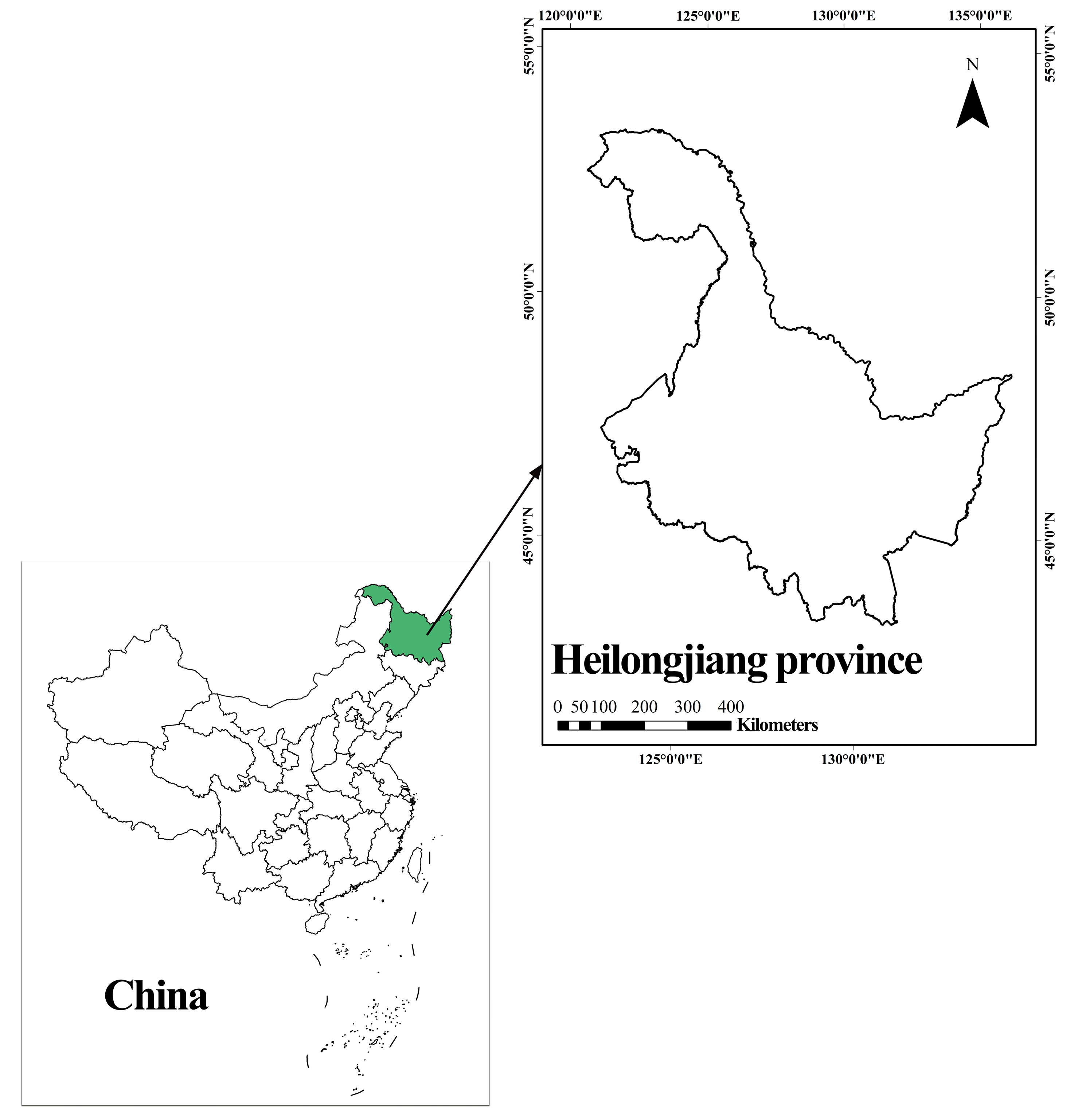
Figure 1. Map of the region of study in Heilongjiang Province, China.
Remotesensing 15 04197 g001
Figure 2. GPP of the annual growing season in Heilongjiang Province, China, calculated by different remote sensing products.
Remotesensing 15 04197 g002
Figure 3. Annual average CO2 concentration in Heilongjiang Province, China.
Remotesensing 15 04197 g003
Figure 4. Nitrogen deposition (Ndep) of the annual growing season in Heilongjiang Province, China (a). Average temperature (Tmean) of the annual growth season in Heilongjiang Province, China (b). Precipitation of the annual growth season in Heilongjiang Province, China (c). Average water vapor pressure difference (VPD) of the annual growth season in Heilongjiang Province, China (d).
Remotesensing 15 04197 g004
Figure 5. Stand age distribution map in Heilongjiang Province in 1982 (a). Distribution map of coniferous and broad-leaved forests in Heilongjiang Province (b). Site class index (SCI) distribution map in Heilongjiang Province (c).
Remotesensing 15 04197 g005
Figure 6. Ranking of variable importance for the two remote sensing datasets (a). Comparison between the annual growing season GPP from the random forest model and the annual growing season GPP from the EC-LUE GPP and NIRv GPP datasets (b).
Remotesensing 15 04197 g006
Figure 7. Estimating the CO2 fertilization effect (CFE) trend with age in broad-leaved forests (BF) using EC-LUE GPP (a) and NIRv GPP (b). Estimating the CFE trend with age in coniferous forests (CF) using EC-LUE GPP (c) and NIRv GPP (d).
Remotesensing 15 04197 g007
Figure 8. Estimating the CFE trend with age in CF and BF using the average of two datasets (a). Comparison of CFE in different stand types. Boxes represent the interquartile range of the β values (solid lines represent medians, and empty rectangles represent the average value). The upper and lower extension lines extend to 1.5 times the interquartile spacing (b).
Remotesensing 15 04197 g008
Figure 9. Spatial distribution of CFE in Heilongjiang Province, China.
Remotesensing 15 04197 g009
Figure 10. Differences in the CFE among different site quality levels. Different letters in each bar indicate significant differences (p < 0.05), and error bars represent the 95% confidence interval (a). The decline rate of CFE with age across different site levels (b).
Remotesensing 15 04197 g010
Table 1. Description of the data used in this study.
DatasetDescriptionResolution
EC-LUE GPP1982–2017 global GPP dataset corrected using the EC-LUE model0.05° × 0.05°; 8-day
NIRv GPP1982–2018 global GPP dataset estimated using novel vegetation index NIRv0.05° × 0.05°; monthly
CO2 concentrationData on annual average atmospheric CO2 concentrations from 1982 to 2010 published by the Mauna Loa Observatory—ESRL Global Monitoring LaboratoryYearly
Nitrogen deposition (Ndep)The historical nitrogen deposition database (1850–2014) in the input4MIPs dataset0.5° × 0.5°; monthly
Climatic dataCalculated from the CRU TS (version 4.0.5) global meteorological data from 1901 to 2020 provided by the National Centre for Atmospheric Science0.5° × 0.5°; monthly
Stand age mapConstructed from forest inventory data in 20101 km × 1 km
Stand type mapConstructed from CAS in 20061 km × 1 km
Site class index mapConstructed from forest inventory data in 20101 km × 1 km
Table 2. The four regression coefficients across different datasets.
Stand Type—Remote Sensing Productabcd
BF-EC-LUE108.522.676.930.76
BF-NIRv63.665.6614.520.85
CF-EC-LUE75.305.1914.580.79
CF-NIRv91.593.447.511.36
BF89.493.4711.280.71
CF81.254.5312.870.91
a, b, c, and d are nonlinear regression model coefficients in Equation (8).
Disclaimer/Publisher’s Note: The statements, opinions and data contained in all publications are solely those of the individual author(s) and contributor(s) and not of MDPI and/or the editor(s). MDPI and/or the editor(s) disclaim responsibility for any injury to people or property resulting from any ideas, methods, instructions or products referred to in the content.