Abstract
Radiative transfer model (RTM) simulated microwave (MW) brightness temperatures (Tbs) are commonly used to monitor and evaluate space-based MW sensor-observed antenna temperature (Ta) data. Although these simulated Tbs are paramount to this data integrity maintenance activity, their uncertainties have not been quantified. This study develops and implements a method to estimate these simulated Tb uncertainties based on a statistical comparison of two Community RTM (CRTM)-simulated operational MW sounder Tb data sets, separately generated using the European Center for Medium Range Forecasts (ECMWF) Atmospheric Model High Resolution (HRES) and Global Navigation Satellite System (GNSS) Radio Occultation (RO) sounding inputs. The study shows the smallest single-sensor CRTM-simulated Tb uncertainties, computed from differences of ECMWF HRES and GNSS RO soundings-based simulated Tbs data sets, are on the order of 10−4 relative to a 300 K Tb for the two NOAA operational MW sounder channels with low- to mid-tropospheric peak weighting function sensitivity. Meanwhile, inter-sensor-simulated Tb differences, computed from the double difference of single-sensor-simulated Tb differences, lead to CRTM-simulated Tb uncertainties on the order for 10−4 for at least nine MW sounder channels with peak sensitivity from the low-troposphere to the low-stratosphere. These findings provide the basis of future work to assess the ability to identify and quantify suspected on-orbit MW sounder calibration anomalies using RTM-driven, on-orbit MW instrument monitoring techniques.
Keywords:
satellite microwave remote sensing; remote sensing; Joint Polar Satellite System; Advanced Technology Microwave Sounder; Advanced Microwave Sounding Unit; data performance monitoring; data quality tracking; calibration anomaly detection; radiative transfer model; data simulation uncertainties 1. Introduction
The Advanced Technology Microwave Sounder (ATMS) and Advanced Microwave Sounding Unit (AMSU)-A satellite instruments have been critical in improving numerical weather prediction (NWP) [1,2], earth-system environmental monitoring [3], and extending the long-term mid-tropospheric temperature climate time series of the Microwave Sounding Unit (MSU) [4,5,6,7], the predecessor instrument of AMSU-A and ATMS. The history of AMSU-A and ATMS radiometers used operationally by the National Oceanic and Atmospheric Administration (NOAA) are listed in Table 1. The table shows that the AMSU-A radiometer has been manifested on the NOAA Polar Operational Environmental Satellite (POES) and EUMETSAT Polar System (EPS) Meteorological Operational (Metop) satellite platforms. Meanwhile, ATMS has been manifested on the NOAA Joint Polar Satellite System (JPSS) and Suomi National Polar Partnership (NPP) satellite platforms.

Table 1.
NOAA operational MW sounder instrument name, satellite platform, operational (ops) start date, orbit LTAN on the ops start date, orbit drift maintenance and July 2022 status, i.e., Ops or Decom (decommissioned).
From Table 1, it is important to note each satellite is initially placed in either an afternoon or morning orbit with a local time of the ascending node (LTAN) of about 1330–1400 or 1930–2130, respectively. The POES satellites can have an LTAN that changes, since their orbits are not actively maintained, while the EPS, NPP and JPSS satellites have orbits where the LTAN is carefully maintained. As of this writing, the NPP and NOAA-20 satellites are separated by a half-an-orbit in the same orbital plane, so direct inter-comparison of the ATMS microwave (MW) sounders is not possible. The Metop AMSU-A instruments also cannot be directly compared, as at the beginning of 2020, the three Metop satellites shared the same orbit separated by approximately a third of an orbit, and after the summer of 2020 Metop-C was relocated to be approximately half an orbit apart from Metop-B, with Metop-A between the other Metop satellites in preparation for its decommissioning. All other satellite pairs have slightly different orbits from each other, which facilitates periodic simultaneous observations between MW instruments, but only in the polar regions.
In order to utilize these satellite data without the risk of significant uncertainties, inherent calibration-related antenna temperature (Ta) biases and bias trends within and between operating AMSU-A and/or ATMS instruments must be detected and corrected. Thus, monitoring and maintaining the quality of NOAA operational MW radiometer data are critical to ensuring that NOAA meets its mission of atmospheric- and oceanic-related science, service and stewardship for the United States. On the other hand, monitoring passive MW sounder instruments and data performance has many notable challenges.
Earth scene emission in the MW spectrum between 23 GHz and 60 GHz is rarely stable, thus the dynamic radiometric character of a given region of interest must be well understood before it can be used as a MW instrument validation target. In the 18 GHz to 40 GHz region, the Amazon Rainforest is an Earth region that has been extensively documented as a validation target for MW sounder channels, e.g., Brown and Ruf [8]. Such methods though are often limited by the hour of the day and season. There are no such Earth validation targets for MW sensor channels between 40 GHz and 60 GHz. So, to be able to monitor these channels, a reference standard needs to be established that is capable of removing at-sensor MW sounder measurement changes distinctly associated with Earth surface and atmospheric state variability.
A widely accepted method to do this is to assign radiative transfer model (RTM)-simulated background at-sensor brightness temperatures (Tbs), generated where there are collocated atmospheric temperature and moisture soundings and MW sounder measurements, as a reference. This method entails the simple comparison of instrument-observed (O) Ta (or Tb) values with respect to simulated background (B) Tb to produce O-B Ta biases. In order to implement this method in clear-sky regions, atmospheric sounding data that include pressure, temperature, water vapor mixing ratio, and ozone mixing ratio are needed to establish representative internal conditions for the RTM.
Application of this method to the NPP ATMS using the National Centers for Environmental Prediction (NCEP) Global Forecast System (GFS) 6-hr forecast outputs can be found in a paper by Weng et al. [9]. Iacovazzi et al. [10,11] implemented this method by harnessing the Constellation Observing System for Meteorology, Ionosphere, and Climate/Formosa Satellite Mission 3 (COSMIC-1/FORMOSAT3, hereafter referred to as COSMIC-1 for brevity) and COSMIC-2 Global Navigation Satellite System (GNSS) Radio Occultation (RO) sounding data to establish internal conditions for the Community Radiative Transfer Model (CRTM). These studies shed light on the usefulness of this method for detecting MW sounder anomalies.
A physical framework using radiance units can explain how satellite MW instrument observations are evaluated using single-sensor O-B Ta biases and their inter-sensor double differences. Radiance is adopted here, because ATMS instrument calibration is performed in radiance units before being transformed to Ta and Tb data products. The radiance and Ta/Tb units will be used interchangeably in this study though, with the understanding that they are related through Planck’s law.
In the radiance domain, the O-B Ta bias values can be derived from the simulated Earth (E) scene background radiance, ; which is composed of the RTM antenna main beam (MB) Earth scene radiance, ; antenna sidelobe (SL) Earth scene radiance, ; SL cosmic background radiance, ; and model uncertainties, . This can be expressed as:
The nearly-circular antenna MB boundary is defined as 2.5 times the elevation angle of the antenna response half-power point, relative to the antenna boresight. Meanwhile, the antenna response SL region is the remaining solid angle beyond the antenna MB boundary.
Ideally, the RTM outputs a Tb for the region subtended by the antenna MB response. So, there are no simulated contributions from the antenna SL regions. This inherently makes observed Ta and simulated Tb physically unequal quantities. By comparing observed Ta and RTM-simulated Tb, the simulated antenna MB radiance field unavoidably becomes extended to the antenna SL regions. As a consequence, there is a non-negligible overestimate for the cold space radiance in the antenna SL regions, , and in turn a persistent RTM-simulated Tb value warm bias is present when compared to observed Ta.
The microwave sounder-observed Earth radiance, , is composed of scene radiance from the antenna MB, , and Earth and cosmic background contributions through the antenna SL regions, and . These radiometric contributions are assumed to be acquired from a “perfect” radiometer, and the observation uncertainty contributions related to all terms are all captured in the term, . This can be expressed as:
The difference of the observed and simulated MB Earth scene radiance for a single MW sensor is given as follows:
The three elements in parentheses on the right-hand side of the equation represent the differences of the observed and simulated radiances in the MB and SL regions. The remainder of the terms on the right-hand side represent terms associated with observation and radiative transfer model simulation uncertainties.
The inter-sensor radiance difference is given by a similar equation:
There are no accounts that determine the statistical significance of the estimated O-B Ta biases, because RTM-simulated Tb uncertainty estimates have not been established. In Equations (3) and (4), it becomes clear that not having knowledge of the simulated MW measurement uncertainty characteristics could become problematic in determining the significance of the single-sensor difference between the observed and simulated MW measurements and their inter-sensor double differences. The present study established a method to estimate RTM-simulated Tb uncertainties. These uncertainty results could be used to assess their impact on the fidelity of the MW sensor monitoring systems. They also could open the door to further investigation into the possibility of using such monitoring systems to detect, assess, understand and mitigate MW sensor anomalies.
In the next section, we briefly describe the AMSU-A and ATMS instruments and their data, the CRTM, and the European Centre for Medium-Range Weather Forecasts (ECMWF) Atmospheric Model High Resolution (HRES) 10-day forecast and COSMIC GNSS RO atmospheric soundings. The section also discusses the method to determine CRTM-simulated Tb uncertainties for single MW sensors and inter-sensor MW instrument pairs, while Section 3 provides the resultant uncertainty estimates. Finally, in Section 4, a general discussion of the results, and the research path forward, are provided.
2. Materials and Methods
2.1. Instruments, Models and Data
Since previous literature exists regarding the instruments, models and data relevant to this study, references are provided in the following subsections to open source articles that describe the key features of these assets. Details will be added in the subsections only when they are not addressed in the references and are important and relevant to the study.
2.1.1. NOAA Operational Microwave Sounding Radiometers
The NOAA operational satellite ATMS Channels (Chs) 2, 3, and 5–15 (AMSU-A Chs 2–14) O-B Ta bias statistics, supported by GNSS RO soundings, are monitored and evaluated within the NOAA/NESDIS Center for Satellite Applications and Research (STAR) Integrated Cal/Val System (ICVS). However, a persistent limitation of this monitoring system has been the lack of estimated CRTM-simulated MW Tb uncertainties. The goal of the current study is to eliminate this limitation. In achieving this goal, no NOAA operational MW sounder Ta observations are used at all, but this research does utilize the associated MW observation time stamp and geolocation data to temporally and spatially collocate the NOAA operational MW sounder data samples to the GNSS RO soundings. This process strictly confines the CRTM-simulated Tb uncertainties to only the population of GNSS RO soundings associated with MW sounder observations.
Even though an in-depth introduction into the NOAA operational satellite ATMS and AMSU-A instruments is not necessary, readers who wish to become more familiar with the instruments and their calibration may refer to several articles [12,13,14,15]. These articles discuss the ATMS and AMSU-A characteristic channel numbers, center frequencies, bandwidths, polarizations, nominal beamwidths, nadir beam sizes and weighting functions at nadir. They also include information on instrument channel accuracy and NEDT specifications, calibration processes, cross-track data sampling and total swath width.
2.1.2. The CRTM and Its Internal and Boundary Condition Input Sources
The CRTM used in this study is publicly available and may be downloaded from https://ftp.emc.ncep.noaa.gov/jcsda/CRTM/REL-2.1.3/ (accessed on 16 August 2023). It is developed and distributed by the US Joint Center for Satellite Data Assimilation (JCSDA) and widely used for microwave and infrared satellite data assimilation and remote sensing applications. The CRTM is a sensor-channel-based radiative transfer model [16,17,18,19]. It has integrated portions that compute the satellite-measured thermal radiation from gaseous absorption, absorption and scattering of radiation by aerosols and clouds, and emission and reflection of radiation by the Earth’s surface. The CRTM input parameters include atmospheric temperature, water vapor, pressure, and ozone concentration at user-defined layers. It also includes optional input variables and parameters, such as liquid water content and mean particle size profiles for up to six cloud types, and surface emissivity, skin temperature and wind.
In this study, the vertical profiles of temperature, water vapor and pressure are obtained from COSMIC GNSS RO retrievals and ECMWF HRES model output, and near-surface wind speeds are assigned climatological values. More information about these inputs is provided below. The U.S. Standard Atmosphere 1976 ozone mixing ratio profile is assumed, and no clouds or aerosols are considered, in the radiative transfer simulations. The emissivity is derived from the CRTM oceanic surface model at MW frequencies.
The GNSS RO soundings are based on estimates of atmospheric refractivity as a function of altitude from the Earth’s surface. This refractivity estimate depends on temperature, water vapor, and pressure in the neutral atmosphere [20]. The present study uses available COSMIC-1, COSMIC-2 and Korean Multi-Purpose Satellite-5 (KOMPSAT-5) wetPrf retrieval products from 1 January 2020 to 31 December 2020 to support CRTM MW sounder Tb simulations. Note that the COSMIC-1 service ended on 25 April 2020.
In Table 2, we provide information about each of these GNSS RO programs, including the number of sensors, orbit apogee/perigee and inclination, Earth coverage, number of samples per day, sounding vertical/horizontal resolution and elevation cutoff. The COSMIC-1 and KOMPSAT-5 wetPrf product is downloaded from the COSMIC Data Analysis and Archive Center (CDAAC), while the COSMIC-2 wetPrf sounding data are obtained from the STAR GNSS RO Team. The 1D-Var algorithms used to produce these products are compatible [21,22,23].

Table 2.
GNSS RO programs, including the number of sensors, orbit apogee/perigee and inclination, Earth coverage, number of samples per day, sounding vertical/horizontal resolution and elevation cutoff.
Atmospheric temperature predominantly determines refractivity between 8 km and 30 km, so this layer has the lowest sounding uncertainties of about 0.7 K [24,25]. Meanwhile, COSMIC-1 GNSS RO inter-sensor uncertainty relative to closely collocated Challenging Minisatellite Payload (CHAMP) and Scientific Application Satellite-C (SAC-C) GNSS RO soundings is approximately 0.05 K in the upper troposphere and lower stratosphere [26]. The COSMIC-2 measurement accuracy between 8 km and 30 km has been determined by Ho et al. [27], which is largely in-family with COSMIC-1. In the atmospheric regions below and above this layer, there are greater sounding uncertainties. This is because refractivity depends on both temperature and water vapor concentration below 8 km, and both temperature and ionosphere density distribution above 35 km.
The ECMWF HRES forecast is run every six hours out to 10 days with a native horizontal resolution of 18 km and 137 layers in the vertical. The output soundings from these forecasts are degraded to a 0.25° × 0.25° longitude and latitude grid, and to 91 levels in the vertical between the surface and 80 km, before they are distributed to NOAA/NESDIS/STAR.
For the GNSS RO soundings, the gap between the minimum sounding level and the Earth’s surface is usually relatively small (<0.5 km), but there still can be a noticeable temperature disparity. Thus, to estimate the Earth’s surface temperature, a dry adiabatic profile is assumed to be able to extrapolate atmospheric temperature to near the surface. It is then further assumed that this near surface temperature is the same as the Earth’s skin temperature. Meanwhile, the ECMWF HRES temperature and water vapor soundings are adequately resolved in the boundary layer without need for extrapolation.
Blended ocean wind speed and direction climatology monthly datasets with a 0.25° resolution are used to support sea-surface microwave emissivity estimation in the CRTM. The wind speed climatology data are the NOAA Multiple-Satellite Blended 0.25° Sea Winds—climatological monthly means. This climatology is derived from multiple satellite observations: Defense Meteorological Satellite Program (DMSP) Special Sensor Microwave Imager (SSMI) F08, F10, F11, F13, F14, and F15; NASA Tropical Rainfall Measurement Mission Microwave Imager (TMI); QuikSCAT; and the JAXA AMSR-E. The wind direction climatology is based on the NCEP Reanalysis-2. See https://www.ncei.noaa.gov/products/blended-sea-winds (accessed on 16 August 2023) and links within for details.
2.2. Methods to Collocate GNSS RO and ECMWF HRES Soundings and Estimate Simulated MW Tb Uncertainties
The methods that support the estimation of CRTM-simulated Tb uncertainties are presented here. The first sub-section describes how the GNSS RO and ECMWF HRES soundings are collocated at MW instrument data locations and timestamps. The second sub-section describes how the collocations are used as the basis for simulating Tbs separately with GNSS RO and ECMWF HRES soundings for each MW instrument, and how these simulated Tbs are analyzed to determine CRTM-simulated MW Tb uncertainty.
2.2.1. Collocating GNSS RO and ECMWF HRES Soundings at MW Sensor Data Locations and Timestamps
In this study, the word “collocate” or “match” defines the process of determining that measurements from two data sources are within a certain proximity to each other by using a set of imposed time and distance difference limits. The word “interpolate” means to create an estimate of the values of one data set at the sample times and/or locations of another data set. The GNSS RO time and lat/lon data represent the temporal and spatial anchor to which the MW sensor data samples and ECMWF HRES soundings are collocated and/or interpolated. Note again that no NOAA operational MW sounder Ta observations are used in this study. The MW sounder observation time stamp and geolocation data are used to temporally and spatially collocate the MW sounder data samples to the GNSS RO soundings. This is performed to ensure that the estimates of the CRTM-simulated Tb uncertainties are restricted to GNSS RO soundings associated with MW sounder observations. The data flow illustration for this is depicted in Figure 1, and more details are given in the following.
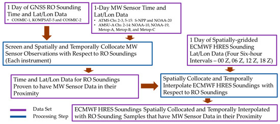
Figure 1.
The high-level depiction of the data flow for ECMWF HRES soundings spatially collocated and temporally interpolated with GNNS RO soundings samples that have MW sensor data in their proximity.
A single day of COSMIC and KOMPSAT-5 GNSS RO atmospheric temperature and moisture soundings are imported from the CDAAC and NOAA/NESDIS/STAR data sources mentioned earlier. Data are limited to those samples falling equatorward of 60° latitude. A day of geolocation and timestamp data from a given MW sounder is also imported to determine the population of GNSS RO soundings that have Ta data samples associated with them. The time and space difference collocation criteria between a given GNSS RO sounding and each MW radiometer data sample is prescribed to be no more than three hours and less than 50 km, respectively. Note that the collocation process considers the weighting function peak altitude for each MW sensor channel and scan position. This step isolates those GNSS RO soundings that have MW sounder observations in proximity to them.
The ECMWF HRES soundings are on a 0.25° × 0.25° and 6-h space and time grid, respectively. For each of the isolated GNSS RO soundings, the ECMWF HRES model statistics for the two time periods bounding the GNSS RO observation time are obtained. Then, for the ECMWF model grid point lat/lon nearest to the GNSS RO sample lat/lon, the two ECMWF HRES soundings from the two bounding time periods are interpolated to the GNSS RO observation time. This creates one ECMWF HRES sounding spatially collocated and temporally interpolated with an RO sounding sample that has MW sensor data in its proximity. This is performed for all of the isolated GNSS RO soundings that are found to match in space and time with data from each of the MW sensors.
For identified matched pairs, the sounding quality is further screened. This screening process attempts to minimize MW surface emissivity uncertainties, and MW signal impacts caused by hydrometeor scattering effects. For example, ATMS(AMSU-A) Chs 2–3 and 5–6(Chs 2–5), which have sizable surface radiance transmittance, are limited to ocean regions only and are screened for clouds using a method similar to Weng et al. [28]. Meanwhile, ATMS Chs 7–15 and AMSU-A Chs 6–14 that are negligibly influenced by surface emissions are screened out only for land regions with elevations higher than 2 km. Overland precipitation identification and rejection is carried out using the method of Grody et al. [29].
Additional GNSS RO screening techniques applied in this study include rejecting soundings that have greater than 360 km maximum sounding measurement Earth location variation with altitude. Also, soundings are rejected if they do not have adequate depth to produce meaningful radiative transfer model simulations. For MW sensor channels with high surface radiance transmittance through the atmosphere—e.g., ATMS(AMSU-A) Chs 2–3 and 5–6(Chs 2–5)—the GNSS RO soundings must have valid data down to 1000 mb. For all other channels, it is important for a sounding to extended deep enough in the atmosphere to capture the thermodynamic state of the layer where at least 95% of the plausible MW signal reaches the sensor. More detailed information about these screening techniques can be found in Iacovazzi et al. [11].
The resulting data set of GNSS RO and ECMWF HRES soundings that have MW sounder observations in proximity to them forms the foundation for the CRTM-simulated Tb uncertainty analysis. Since the GNSS RO and ECMWF HRES soundings inherently have time offsets and spatial dimension differences, some variability between these soundings will be apparent after interpolation. The magnitude of this variability largely depends on the nature of spatial and temporal meteorological variability, and the GNSS RO and ECMWF HRES sounding resolution differences. This variability will cascade into the overall uncertainty between the Tbs simulated using the GNSS RO soundings and those simulated using the ECMWF HRES soundings. This impact on uncertainty for a large population of measurements is very difficult to isolate unequivocally, and is not determined in this study.
2.2.2. Estimating CRTM MW Tb Simulation Uncertainties
CRTM-simulated radiance uncertainty, , that translates into simulated Tb uncertainty, is assumed to have two primary contributions. The first is incomplete and/or inadequate radiative transfer solver and surface emissivity physics, and the second is input atmospheric profile uncertainties. In the following, we summarize previously documented evidence of Tb uncertainties related to incomplete and/or inadequate CRTM physics. Then, an approach is described to determine uncertainties related to input atmospheric profile uncertainties from the set of GNSS RO and ECMWF HRES soundings in proximity with MW sensor data times and locations.
It is important for radiative transfer models not only to be accurate, but also to be as fast as possible, since they are used for real-time operational applications such as weather forecasting and environmental monitoring. To fulfill this need, the CRTM has made approximations or truncations to more physically rigorous, and computationally intensive radiative transfer and surface emissivity estimation schemes. For example, the Doubling Adding (DA) radiative transfer solver has been simplified to significantly economize the radiative transfer solution in the Successive-Order-of-Interactions (SOI) solver by Heidinger et al. [30] and O’Dell et al. [31], and the Advanced Doubling Adding (ADA) solver by Liu and Weng [32]. For the SOI solver, this computational economy results in less than 0.03 K error relative to the DA solver for precipitation-related single-scattering albedo less than 0.8 and optical depth less than 3 for MW channels between 10 GHz and 37 GHz. Similar results are found for the ADA solver. This means that the radiative transfer solution produces very little error when performing Tb simulation in cloud-free regions, as is achieved in this study. It is not expected that there would be more error for 50+ GHz channels within the 60 GHz oxygen absorption band, since these channels can be less impacted by precipitation than window channels.
The FASTEM4/5 surface emissivity model by Liu et al. [33], on the other hand, can have up to 3% uncertainty (~10 K) in some extreme cases. For this study though, impacts of surface emissivity model errors on the total uncertainty of CRTM-simulated Tbs are greatly diminished due to several factors. One factor is that ATMS(AMSU-A) Chs 5–15(Chs 4–14), i.e., 11 of the 13 channels examined in this study, are sounding channels that receive a bulk of their radiance from the atmosphere, and not the surface. For land scenes, the analysis is further restricted to ATMS(AMSU-A) Chs 7–15(Chs 6–14), and these channels receive less than 1% of their radiance from the surface. So, a worst-case error would be only 0.1 K. The most significant impacts of surface emissivity uncertainty are found for ATMS/AMSU-A window channel Tb simulations over ocean scenes.
For ocean scenes, window Ch 2 [31.4 GHz] and Ch 3 [50.3 GHz] can have significant surface emissivity errors caused primarily by input wind speed/direction errors. This study assumes climatological wind speed/direction over ocean scenes, so when the climatological wind speed/direction is much different than the actual, surface emissivity errors can produce those 10 K Tb errors. On the other hand, over time and a large spatial region, variability in wind speed/direction average out to a small bias that effects only these window channels. We make it a point in this paper to discuss the errors related to our assumptions about wind speed/direction and their effects on CRTM-simulated ATMS(AMSU-A) Ch 2 and 3 Tb. It also needs to be noted that surface emissivity errors will not be detectable when comparing two Tb simulations generated with different soundings. This is because the simulations share the same emissivity model and climatological wind speed/direction. So, any surface emissivity impacts cancel in the difference between the two simulated Tbs. From this summary of previous work, and assumptions regarding this analysis, cloud-free regions have very little error due to the CRTM physics, but the internal conditions of the model, i.e., the input temperature and moisture soundings, may introduce much larger uncertainties to CRTM-simulated Tb.
CRTM simulations based on atmospheric temperature profiles derived from GNSS RO refractivity data are independent of the MW radiometer data. Moisture profile creation from RO refractivity data though needs support from MW-data-rich NWP model soundings, but this is mainly in the low- to mid-troposphere where there can be abundant water vapor content. The ECMWF HRES temperature and moisture soundings represent the assimilation of many diverse data sources that include aircraft, radiosonde, space-based IR/MW sounder and GNSS RO data. So, GNSS RO soundings by themselves do not necessarily correlate with the ECMWF HRES soundings.
The approach used to estimate CRTM-simulated Tb uncertainties is to first categorize the GNSS RO and ECMWF HRES temperature and moisture soundings that are in proximity with MW sensor data samples by region-of-interest (ROI). These ROIs include the global region between 60°S and 60°N, and several smaller ROIs, e.g., ocean and land surface types; tropical, subtropical, and mid-latitude latitude bands; and ascending and descending satellite orbit nodes. This is performed using data for the time period from 1 January to 31 December 2020. Then, GNSS RO and ECMWF HRES temperature and water vapor soundings are averaged separately over each of these eight ROIs for each MW sensor. These separately averaged GNSS RO and ECMWF HRES soundings are then used as input into the CRTM.
Each set of separately averaged GNSS RO and ECMWF HRES temperature and moisture soundings for each MW sensor can be used to generate CRTM-simulated TbRO and TbEC data sets, respectively. For this study, the simulated Tb values for the ATMS and AMSU-A sensors are calculated at all 96 ATMS instrument scan angles, which allows for a “per-scan-angle” analysis of the uncertainty and aids comparison between ATMS and AMSU-A results. Then, for each MW sensor, these simulated TbRO and TbEC data sets can then be compared statistically to understand the bias and variability between them, which is assumed to stem from bias and variability between the GNSS RO and ECMWF temperature and water vapor soundings.
The CRTM-simulated Tb single sensor (SS) uncertainties are founded on the difference of Tbs simulated with the ECMWF HRES soundings and those simulated with the GNSS RO soundings for the matchups corresponding to a single instrument. For a given day, these data produced from matchups in the defined ROIs can be analyzed to generate daily regional-mean SS CRTM-simulated Tb difference, , values. For the time period from 1 January to 31 December 2020, the time series of values in each ROI and their time series mean, , and standard deviation, , statistics can be computed at each scan angle, and used as estimates of CRTM-simulated Tb uncertainties for a single satellite. The double difference of the results from pairs of MW sensors for each day and region can be computed to estimate the CRTM-simulated Tb inter-sensor (IS) uncertainties, , at each scan angle. Similar time series statistics produced for can also be computed for values. A data flow of this full data process is summarized in Figure 2.
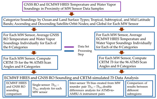
Figure 2.
The flows of processing and analysis of the GNSS RO and ECMWF HRES temperature and water vapor soundings collocated at MW sensor data samples.
The estimate of the single-sensor and inter-sensor Tb uncertainty is based on the root mean square error (RMSE) statistic, which is given as:
where XX can be SS or IS. The parameter n is the sample number, and N is the total number of samples, which will be clarified later for each implementation of the equation. These uncertainties can then be used to create a Normalized Scaling Factor (NSF) value that can be used to quickly determine the relative magnitude of a given uncertainty. The NSF value is defined in this work as the fraction of a given uncertainty relative to a 300 K blackbody source, which can be deduced from as:
where and . For example, if a value of uncertainty is 0.487, then X = 1.623 × 10⁻³ and α = 0 and NSF = 10−3.
3. Results and Discussion
The following three subsections are structured in a manner that illuminates the reasons why there are CRTM-simulated Tb uncertainties, and estimates the magnitude of these uncertainties.
3.1. Average ECMWF HRES and GNSS RO Temperature and Water Vapor Soundings and Their Differences
The ECMWF HRES and GNSS RO full-atmospheric depth temperature and moisture soundings are used as a basis to estimate the CRTM-simulated Tb uncertainties. Thus, providing examples of these sounding and their differences can provide insights into possible impacts they have on the simulated Tb values. In Figure 3a,b, the mean of ECMWF HRES and GNSS RO sounding temperature averaged over the global region between 60°S and 60°N for all collocations with Suomi NPP (NPP) and NOAA-20 (N20) ATMS and NOAA-18 (N18), NOAA-19 (N19), Metop-A (MEA), Metop-B (MEB) and Metop-C (MEC) AMSU-A are shown for 1 January and 1 July 2020, respectively. The troposphere, tropopause, stratosphere, stratopause and lower mesosphere are clearly identifiable in both figures. The tropopause is visibly higher and cooler, and the stratopause warmer, in January compared to July. The difference between the ECMWF HRES and GNSS RO sounding temperature averaged over the same region and days is shown in Figure 4a,b. These figures show that the temperature differences are significant throughout the stratosphere and the maximum difference in the mesosphere is larger and lower in the atmosphere in January compared to July. Also, noticeable variability of as much as 100% between instruments, especially on 1 July 2020, becomes visibly apparent above about 25 km. The cause of this variability is discussed in Section 3.3.
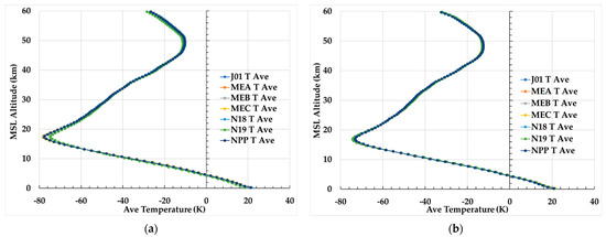
Figure 3.
Mean of ECMWF HRES and GNSS RO sounding temperatures averaged over the region between 60°S and 60°N for all collocations with NPP and N20 ATMS and N18, N19, MEA, MEB and MEC AMSU-A are shown for (a) 1 January and (b) 1 July 2020. Note that the y-axis label “MSL Altitude” denotes Mean Sea Level Altitude.
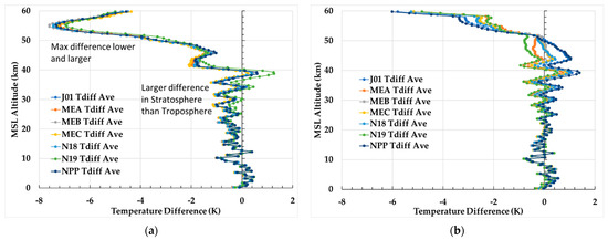
Figure 4.
Difference in ECMWF HRES and GNSS RO sounding temperatures averaged over the region between 60°S and 60°N for all collocations with NPP and N20 ATMS and N18, N19, MEA, MEB and MEC AMSU-A are shown for (a) 1 January and (b) 1 July 2020. Note that the y-axis label “MSL Altitude” denotes Mean Sea Level Altitude.
In Figure 5a,b, similar plots associated with the ECMWF HRES and GNSS RO sounding water vapor pressure values are presented. These figures show a drop-off of water vapor pressure from about 20 hPa near the surface to 0.2 hPa at 9 km. Above 9 km, it drops about another order of magnitude by about 12 km. Also, the peak water vapor pressure near the surface is about 1–2 hPa larger on 1 January 2020 than 1 July 2020. The difference between the ECMWF HRES and GNSS RO sounding water vapor pressure averaged over the same region and days is shown in Figure 6a,b. These figures show that the differences are smaller near the surface in July compared to January. Also, the variability between instruments is only about 10%.
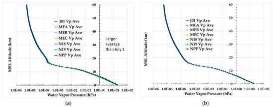
Figure 5.
Mean of ECMWF HRES and GNSS RO sounding water vapor pressure values over the region between 60°S and 60°N for all collocations with NPP and N20 ATMS and N18, N19, MEA, MEB and MEC AMSU-A are shown for (a) 1 January and (b) 1 July 2020. Note that the y-axis label “MSL Altitude” denotes Mean Sea Level Altitude.
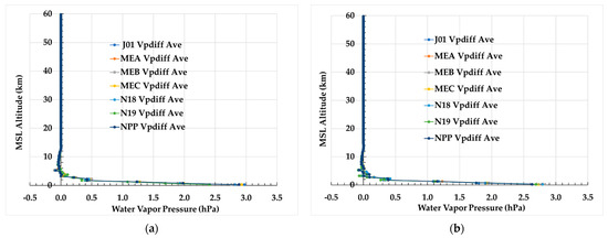
Figure 6.
Difference in ECMWF HRES and GNSS RO sounding water vapor pressure values averaged over the region between 60°S and 60°N for all collocations with NPP and N20 ATMS and N18, N19, MEA, MEB, and MEC AMSU-A are shown for (a) 1 January and (b) 1 July 2020. Note that the y-axis label “MSL Altitude” denotes Mean Sea Level Altitude.
Variability between ECMWF HRES and GNSS RO soundings are shown in these figures to be functions of both season and altitude. The large systematic difference that can occur between these soundings, e.g., in temperature above 40 km and water vapor pressure below 8 km, cannot be explained as an artifact of interpolation. Since MW radiative transfer simulations are rooted in their internal and boundary conditions, these variations will have consequences on the character of the Tbs and their uncertainties. The next section explores this in much more detail.
3.2. Near-Nadir Global-Average CRTM-Simulated MW Sounder , and Time Series and Statistics
Time series of daily near-nadir global-average CRTM-simulated Tb values, produced separately from ECMWF HRES and GNSS RO soundings, are used in this section to reveal the magnitude and variability in simulated Tb measurements, as well as the uncertainties that are manifested between the two data sets. Note that near-nadir in this case is associated with the results from ATMS scan position 49, which only has a 0.555° scan angle with respect to the nadir vector pointing directly below the satellite to the Earth surface. The next three figures showcase near-nadir simulations made using ECMWF HRES and GNSS RO soundings over the “global” region between 60°S and 60°N for all collocations with NPP and N20 ATMS Chs 2, 7, 10 and 15 and N18, N19, MEA, MEB and MEC AMSU-A Chs 2, 6, 9 and 14 between 1 January 2020 and 31 December 2020. We remind the reader that “global” means ocean-only for MW instrument channels that receive significant radiance from the surface, which in this subsection includes ATMS/AMSU-A Ch 2.
In Figure 7a–d, the time series of daily global-average SS CRTM-simulated Tb generated using the ECMWF HRES soundings, , provide the typical Tb values associated with each of these channels at near-nadir. Figure 7a shows that for ATMS and AMSU-A Ch 2 varies between about 153 K and 157 K during the first half of 2020, and between 154 K and 157 K in the remainder of 2020. The relatively low temperature occurs because the “window” channel data used in this study are limited to clear sky ocean, and ocean-surface emissivity in the MW region is about 0.5 to 0.7. The values shown in Figure 7b,c for ATMS/AMSU-A Ch 7/6 (ATMS/AMSU-A Ch 10/9) shows temperature rises from about 241 K (204 K) at the beginning of 2020, and peaks at about 243 K (209 K) in August before sliding back to about 241 K (204 K) by the end of the year. In Figure 7d, has a strong seasonal variability that spans from about 248 K to about 254 K. Variability between instruments in these figures is also evident. This inter-sensor variability could be a consequence of sounding uncertainties associated with satellite orbit differences. This is discussed further in Section 3.3.
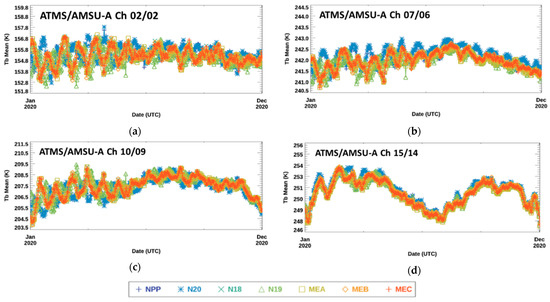
Figure 7.
Time series of daily global-average SS CRTM-simulated Tb from the ECMWF HRES soundings, , at near-nadir. These subfigures have been generated for ATMS/AMSU-A (a) Ch 2/2, (b) Ch 7/6, (c) Ch 10/9, and (d) Ch 15/14 between 1 January 2020 and 31 December 2020. The legend identifying each satellite in the plots is at the bottom of the figure.
The daily global-average SS CRTM-simulated Tb difference, , time series associated with near-nadir pointing instrument scan angle (ISA) number 49 for these MW sensor channels are shown in Figure 8a–d. The most striking feature of the time series is that all instruments have similar trends and variabilities for a given MW sounder channel. The values in Figure 8b,c associated with ATMS/AMSU-A Ch 7/6 and Ch 10/9, respectively, show that the simulations derived from the ECMWF HRES data are cooler than those from the GNSS RO data by about 0.1 K to 0.2 K, and have a min-to-max range of about 0.2 K to 0.4 K. In Figure 8c, there is a jump of about 0.25 K that occurred on about 1 July 2020. Figure 8a,d for ATMS/AMSU-A Ch 2/2 and Ch 15/14, respectively, reveal larger average values and min-to-max range than the other channels. Figure 8a,d show that simulations using the ECMWF HRES data are warmer (cooler) by about 1.26 K (1.70 K) and have a min-to-max range of about 0.6 K (5 K).
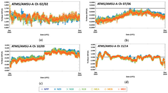
Figure 8.
Time series of daily global-average SS CRTM-simulated Tb difference, , associated with near-nadir ISA 49 for ATMS/AMSU-A (a) Ch 2/2, (b) Ch 7/6, (c) Ch 10/9, and (d) Ch 15/14 between 1 January 2020 and 31 December 2020. The legend identifying each satellite in the plots is at the bottom of the figure.
It is impossible to determine without more information if ECMWF HRES or GNSS RO sounding changes in Figure 8c are the cause of the 1 July 2020 0.25 K jump in . In Figure 9, time series of global monthly mean O-B Ta bias is shown for N20 and NPP ATMS Ch 10 and MEC, MEB, MEA, N19 and N18 AMSU-A Ch 9, created using CRTM-simulated Tb from COSMIC and KOMPSAT-5 GNSS RO soundings that include data from 2020. There are no ECMWF HRES soundings used to generate these time series. These time series do not show a systematic 0.25 K increase starting in July 2020. This is evidence that a change in the ECMWF HRES soundings was the cause of the systematic 0.25 K jump in starting on 1 July 2020, found in Figure 8c.
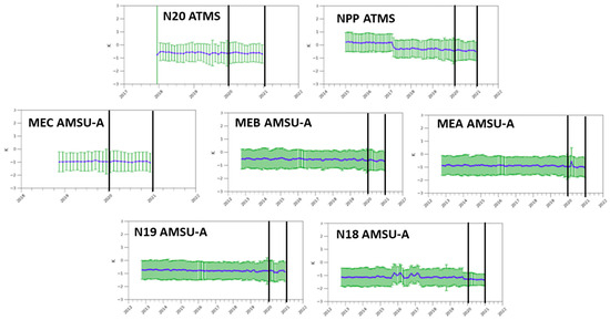
Figure 9.
The global monthly mean (blue curve) and 1-σ standard deviation (green lines) O-B Ta bias time series for ATMS Ch10 from N20 and NPP (top row) and AMSU-A Ch9 from MEC, MEB, and MEA (middle row) and N19 and N18 (bottom row) taken from the STAR Integrated Cal/Val System (ICVS) web site (https://www.star.nesdis.noaa.gov/icvs/ (accessed on 16 August 2023)). The data from 2020 are between the two black vertical lines shown on each plot.
The ATMS-to-AMSU-A inter-sensor daily global-average CRTM-simulated Tb differences, , associated with near-nadir ISA 49 and computed from double differences of the values shown in Figure 8a–d, are presented in Figure 10a–d. Note that the time series for the ATMS-to-ATMS and AMSU-A-to-AMSU-A data are not shown here, but their time series average and standard deviation statistics will be discussed in Section 3.3. Figure 10a–d reveals that most of the seasonal variability present in the time series for a given MW sounder channel is removed in the double difference values. In these figures, the time series mean values do not exceed 0.05 K, and min-to-max ranges are less than 1.0 K. Thus, the double difference eliminates most of the anomalous features from the CRTM-simulated Tbs due to sounding biases. It is not possible from this figure though to speculate about the subtle impacts of inter-sensor differences, such as the LTAN difference between satellites, on daily or .
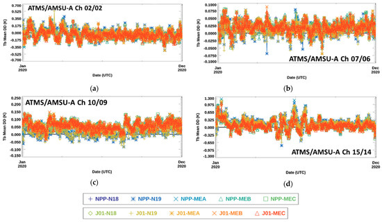
Figure 10.
The time series computed from the ATMS-to-AMSU-A double differences of the time series shown in Figure 8. These subfigures have been generated for ATMS/AMSU-A (a) Ch 2/2, (b) Ch 7/6, (c) Ch 10/9, and (d) Ch 15/14 between 1 January 2020 and 31 December 2020. The legend identifying each satellite pair in the plots is at the bottom of the figure.
The two previous figure groups provide some insight into the behavior of and ATMS-to-AMSU-A over the course of 2020. To further elucidate this insight, the annual population of daily near-nadir global-averages for each time series are used to compute time series mean and standard deviation statistics. This creates a population number, N, of seven single-sensor and ten ATMS-to-AMSU-A matchup pair inter-sensor time series mean and standard deviation values. This population of time series statistics in turn can be used to compute the all-satellite mean (), root mean square (RMS) standard deviation (STD) (), /300 K and NSF values based on and daily statistics associated with near-nadir ISA 49 (note that XX is “SS” or “IS”). These statistics are given in Table 3 for ATMS(AMSU-A) Chs 2, 3, and 5–15(Chs 2–14). Finally, the per-channel statistics are then used to compute the average of the absolute values of these parameters for all 13 channels.

Table 3.
The values of mean (), RMS STD (), /300 K, and NSF derived from the population of seven , and 10 ATMS-to-AMSU-A , time series mean and standard deviation values associated with near-nadir ISA 49 for ATMS(AMSU-A) Chs 2, 3, and 5–15(Chs 2–14).
The all-channel statistics reveal several important analysis details. The average of the absolute values of the means are about six times larger, and the RMS STD values are three times larger, for the single-sensor global daily average CRTM-simulated Tb uncertainties compared to those associated with the inter-sensor double differences. This leads to the number of single-sensor NSF values that are on the scale of 10−4 (10−3) to be 2 (11), while the number of ATMS-to-AMSU-A inter-sensor NSF values at these scales is 11 (2). This clearly shows that the double difference removes much of the CRTM-simulated Tb uncertainties related to ECMWF HRES and GNSS RO temperature and moisture sounding biases.
The CRTM-simulated Tb uncertainties with NSF values of 10−3 and 10−4 relate to uncertainties on the scale of 0.3 K and 0.03 K, respectively. Referring to the accuracy and NEDT specifications for ATMS Chs 2–3 and 5–15 and AMSU-A Chs 2–14 in Table 2 of Iacovazzi et al. [11], if the “accuracy” is considered to be a bias, and “NEDT” is considered to be a standard deviation, then NSF values can be determined from Equations (5) and (6) to describe the uncertainty for the instrument-specified radiometric performance. From this perspective, ATMS Chs 2–3 and 5–12 uncertainty is associated with an NSF value of 10−3 (~0.3 K), while ATMS Chs 13–15 and AMSU-A Chs 2–14 is associated with an NSF value of 10−2 (~3.0 K). This result means that CRTM-simulated Tb uncertainties on the scale of 10−4 do not interfere in single-sensor calibration anomaly analysis related to errors that may exceed specified radiometric performance. On the other hand, CRTM-simulated Tb uncertainties on the scale of 10−3 may introduce uncertainties that compete with single-sensor calibration anomalies for ATMS Chs 2–3 and 5–12. Note that the on-orbit performance of MW sounders can be much better than specified, but an analysis of the impacts of CRTM-simulated Tb uncertainties on single- and inter-sensor calibration anomaly analysis of operational MW sounders is beyond the scope of this paper.
3.3. Annual Regional-Average and Time-Series Statistics
The results of the previous section predict that the near-nadir CRTM-simulated Tb values will not interfere in single-sensor calibration anomaly analysis related to errors that may exceed the specified radiometric performance for ATMS Chs 13–15 and AMSU-A Chs 2–14. However, this encouraging result needs to be investigated with more depth to determine its sensitivity to possible ROI and scan angle differences of CRTM-simulated Tb uncertainties. For this reason, an analysis similar to Section 3.2 is expanded for the data subset (DS) identifiers and classes listed in Table 4. Because of the voluminous output from this analysis, only the time series mean and standard deviation plots are provided. Also, this section is split into three subsections that focus separately on different aspects of the and statistics.

Table 4.
List of data subset (DS) identifiers and classes.
3.3.1. Individual Single-Sensor and Regional-Average Statistics
Figure 11a–d show daily DS-average time series mean, , for ATMS/AMSU-A (a) Ch 2/2, (b) Ch 7/6, (c) Ch 10/9 and (d) Ch 15/14, respectively, during the period from 1 January to 31 December 2020. Systematic differences within a single DS, and from one DS to another, come to attention in these figures. In Figure 11a,b, and d there are two visibly separated bundles of results for each DS. The positive (negative) ATMS/AMSU-A Ch 2/2 (7/6 and 15/14) offset values are related to results from ISA 1 and ISA 96, i.e., ±52.725°. For ATMS/AMSU-A Ch 2/2 and 7/6, the greater water vapor path in the low- to mid-troposphere associated with larger scan angles exacerbates the simulated Tb differences related to the water vapor content biases between GNSS RO and ECMWF HRES soundings shown in Figure 6a,b. For a given instrument, these two channels also show that the mid-latitude region has a smaller bias compared to other regions. This is expected, as the mid-latitude atmosphere on an annual average contains less than half of the atmospheric column water vapor compared to the tropics. For ATMS/AMSU-A Ch 15/14, larger scan angles mean that there is a longer observation path length through the strong GNSS RO warm bias above the stratopause at 50 km. This causes the daily average CRTM Tb biases between those generated by ECMWF HRES and GNSS RO to be more negative for the instrument scan angles that are closer to the Earth limb.
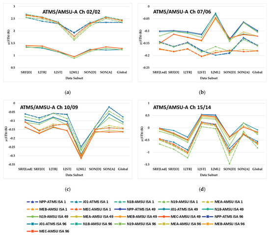
Figure 11.
The values for all surface type, latitude, satellite orbit node and instrument scan angle DS identifier classes given in Table 4. The sub-figures represent ATMS/AMSU-A Ch (a) 2/2, (b) 7/6, (c) 10/9, and (d) 15/14. The legend identifying each satellite and scan position in the plots is at the bottom of the figure.
For ATMS/AMSU-A Ch 15/14, values of can vary by up to 1 K from one DS to another, which is larger than any other channel. This is especially noticeable for L[TR] compared to L[ST] and L[ML], as well as for SON[D] compared to SON[A]. Figure 12 reveals that the average ECMWF HRES and GNSS RO temperature sounding differences of the L[TR] DS compared to the L[ST] and L[ML] DSs, and of the SON[D] DS relative to the SON[A] DS, for N20 can be as large as 7 K above 50 km and −8 K between 30 km and 50 km. Since ATMS/AMSU-A Ch 15/14 is most sensitive to radiance emitted from between 30 km and 55 km, the negative relative bias of L[TR] and SON[D] in this layer is driving the CRTM-simulated Tb differences between subregions.
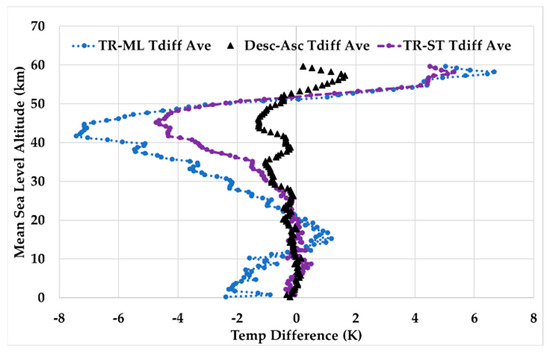
Figure 12.
Difference in ECMWF HRES and GNSS RO sounding temperatures averaged over the L[TR] DS minus those of the L[ST] (purple) and L[ML] (blue) DSs, as well as the SON[D] DS minus the SON[A] (black) DS. This is for all collocations with N20 for 1 January 2020.
The differences between subregions are rooted in differences of atmospheric temperature and water vapor structure. The stratopause for L[ST] and L[ML] is on average higher than L[TR], because it is higher in the polar regions during the polar night [32]. Meanwhile, SON[A] (SON[D]) is distinguished as the sunlit (dark) side of the satellite orbit. Sunlight causes significant global-scale periodic oscillations of the atmosphere that are predominantly associated with effects of solar insolation, e.g., atmospheric ionization in the mesosphere, absorption by ozone in the stratosphere and surface heating and convection in the troposphere. Sounding thermal biases that are evident in Figure 12 between the tropics and mid-latitudes in the lowest 20 km of the atmosphere also drive the simulated Tb bias differences found in L[ML] for ATMS/AMSU-A Ch 7/6.
Figure 13a–d are similar to Figure 11a–d, except that they represent the time series data standard deviation, , instead of the mean, . One feature that is apparent in all figures is a separation between plot groups with smaller and larger . The smaller values are associated with the ISA 49 near-nadir scan angle, while those with larger are derived from ISA 1 and ISA 96 scan angles of ±52.725°. Another anomaly that is present is that the L[ML] region has larger by between 25% and 400% than other regions. The mid-latitudes lie between the poles and tropics. The polar length of day seasonally varies between 0 and 24 h and its surface receives weak or no insolation, while the tropics have nearly 12 h of daylight per day with strong surface insolation all days of the year. This creates meteorological features with pronounced thermal and water vapor spatial and temporal structure variability in the mid-latitudes that represent sharp boundaries between polar and tropical air masses. One final feature to note is the higher values in the L[TR] region for ATMS/AMSU-A Ch 10 and 15/Ch 9 and 14. This increase in may be due to ionospheric variability in the tropical mesosphere which is completely neglected by the GNSS RO algorithm that transforms RO refractivity data into atmospheric temperature.
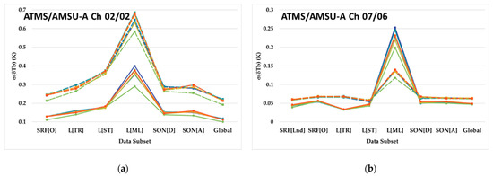
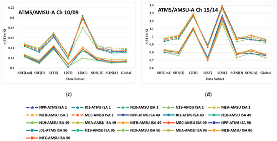
Figure 13.
The values for all surface type, latitude, satellite orbit node and instrument scan angle DS identifier classes given in Table 4. The sub-figures represent ATMS/AMSU-A Ch (a) 2/2, (b) 7/6, (c) 10/9, and (d) 15/14. The legend identifying each satellite and scan position in the plots is at the bottom of the figure.
3.3.2. Individual Inter-Sensor and Regional-Average Statistics
An analysis similar to the one used to generate Figure 11a–d and Figure 13a–d is performed using inter-sensor-simulated Tb difference time series, formed from double differences of the single-sensor-simulated Tb difference time series, as a basis to compute the mean, , and standard deviation, , values. This analysis is carried out only for the near-nadir scan angles, because of the very large double difference data sets. The results shown in Figure 14a–d for and Figure 15a–d for reveal important differences when compared to those in Figure 11a–d and Figure 13a–d, respectively.
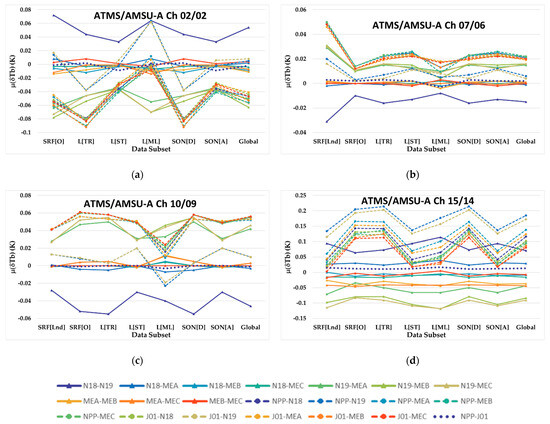
Figure 14.
The values for all surface type, latitude and satellite orbit node DS identifier classes for near-nadir ISA 49. The sub-figures represent ATMS/AMSU-A Ch (a) 2/2, (b) 7/6, (c) 10/9 and (d) 15/14. The legend identifying each satellite pair in the plots is at the bottom of the figure.
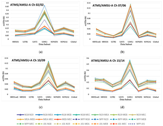
Figure 15.
The values all for surface type, latitude and satellite orbit node DS identifier classes for near-nadir ISA 49. The sub-figures represent ATMS/AMSU-A Ch (a) 2/2, (b) 7/6, (c) 10/9, and (d) 15/14. The legend identifying each satellite pair in the plots is at the bottom of the figure.
Figure 14a–d have min-to-max ranges of values that can be 80% smaller than the min-to-max ranges from Figure 11a–d deduced from the values associated with instrument nadir-only scan angles. The exception to these results is ATMS/AMSU-A Ch 7/6 in Figure 14b, which has a slightly larger (6%) min-to-max range of . The distinct grouping of results in Figure 14a–d is linked to the daily ECMWF HRES and GNSS RO sounding sample subsets being temporally constrained by each satellite’s sun-synchronous polar orbit LTAN, which is turn is associated with diurnal differences between the data populations.
During 2020, NPP and N20 both had a 1330 LTAN, while MEA, MEB and MEC had 2130, 2130, and 2030–2100 LTANs, respectively. Most of these satellites have their orbits maintained, so that the LTAN remains consistent over time. The MEA satellite is an exception, since EUMETSAT stopped maintaining that satellite’s orbit in 2016. The satellite orbits for N18 and N19 were not designed to have their orbits maintained, and thus innately have temporal LTAN drifts. During 2020, N18 had a 2100–2130 LTAN drift, while N19 had a 1745–1815 LTAN drift. Figure 14a–d reflect that the LTAN difference between satellites can impact the CRTM Tb simulation fidelity, since substantial time of day differences can lead to subtle GNSS RO sounding perturbations with respect to the ECMWF HRES soundings (See Figure 12). Based on this reasoning, it is expected that the largest inter-sensor mean biases would be between the ATMS and AMSU-A instruments, and between N19 AMSU-A relative to all other instruments. The smallest inter-sensor biases are expected to be between the NPP and N20 ATMS instruments and between the Metop and N18 AMSU-A instruments. This is exactly what is found. In addition, the magnitude of the DS-to-DS variability in Figure 14a–d also relates to the inter-sensor pairs with the largest satellite LTAN differences.
The results in Figure 15a–d of for surface type, latitude and satellite orbit node analysis DS identifiers and classes for near-nadir ISA 49 manifest behaviors that can also be explained by the satellite LTAN differences. The inter-sensor pairs in Figure 15a–d that have the largest values, and DS-to-DS variances between these values, are the ones that have the largest LTAN differences. Meanwhile, the much larger values related to the L[ML] region can be explained by the relatively large meteorological variability explained in the discussion of Figure 11a–d results.
3.3.3. Bulk Regional-Average and Statistics
The Section 3.2 analysis that led to the results in Table 3 is applied to the seven surface type, latitude, and satellite orbit node DS identifier classes that exclude the global population of simulations. This new analysis generates statistics for ISA 1 and ISA 49, and for ATMS/AMSU-A Chs 2, 3 and 5–15/2–14, and all these channels together. Note that ISA 96 gives identical results to ISA 1, so these redundant results are not generated.
Table 5 shows the all-satellite mean (), RMS STD (), /300 K and NSF values derived from the population of seven single-sensor time series and values associated with all of the above-mentioned DS identifier classes (a population, N, of 49). This table shows the same single-sensor NSF values as Table 3, which was created for the data set that includes the global data for near-nadir ISA 49 scan angle. So, performing the analysis over the smaller DS classes in this case does not have a noticeable impact on single-sensor CRTM-simulated Tb uncertainties. For the Earth limb scan angle at ISA 1 though, there is an increase in all-channel mean and RMS STD of 35% and 13%, respectively, compared to the ISA 49 values. On the other hand, these overall increases in mean bias and standard deviation do not reflect significantly on the NSF values. An NSF value of 10−2 is found for ATMS and AMSU-A Ch 2 for ISA 1, compared to the 10−3 value for ISA 49. Also, ATMS(AMSU-A) Chs 5–6(Chs 4–5) have NSF values of 10−4 for ISA 1, and ATMS(AMSU-A) Chs 6–7(Chs 5–6) have this 10−4 NSF value for ISA 49. This is due to the fact that MW sensors have higher altitude peak weighting functions at Earth limb scan angles compared to near satellite nadir.

Table 5.
Thevalues of mean (), RMS STD (), /300 K and NSF derived from the population of seven individual sensor , and 10 ATMS-to-AMSU-A, 10 AMSU-A-to-AMSU-A, and 1 ATMS-to-ATMS inter-sensor pairs , time series mean and standard deviation values associated with seven surface type, latitude and satellite orbit node DS identifier classes. This analysis has been performed for ISA 1 and ISA 49 and for ATMS/AMSU-A Chs 2, 3, and 5–15/2–14.
The results in Table 5 also show the mean (), RMS STD (), /300 K and NSF values derived from the population of 21 inter-sensor time series and values, from the 10 ATMS-to-AMSU-A, 10 AMSU-A-to-AMSU-A and 1 ATMS-to-ATMS inter-sensor pairs, associated with the seven surface type, latitude and satellite orbit node DS identifier classes that exclude the global population of simulations (a population, N, of 147). When compared to the inter-sensor NSF values shown in Table 3, these results show there are two less 10−4 NSF values for the set of all 21 inter-sensor pairs and 7 DS ROIs compared to the 10 ATMS-to-AMSU-A inter-sensor pairs for the global ROI. This happens for the ATMS and AMSU-A channels that peak in the mid- to upper-stratosphere. There is very little impact shown in Table 5 for the inter-sensor results between the ISA 1 and ISA 49. The exception to this is the all-channel results, which reflects the value being 0.000503 for ISA 1 and 0.000413 for ISA 49. Therefore, there is very little impact of performing the analysis over smaller regions of interest, and over specific scan angle data subsets, on the estimated CRTM-simulated Tb uncertainties.
4. Conclusions
Tracking and maintaining NOAA operational satellite MW sounder data quality is a critical activity supporting numerical weather prediction, near-real time environmental monitoring and climate change investigation. An approach used for this purpose is to generate RTM-simulated satellite MW sensor Tbs where atmospheric temperature and moisture profiles are collocated with MW sounder observations. These simulated Tbs can be subtracted from MW sensor-observed Ta data to produce O-B Ta bias values that can be trended over time. Although this approach has been used for many years to monitor NOAA operational satellite MW sounder data quality, RTM-simulated Tb uncertainty estimates had not been established. Therefore, the magnitude of these uncertainties relative to actual MW instrument calibration anomalies, e.g., antenna emission/absorption and/or cold space view radiance contamination from the Earth and/or spacecraft, within the O-B Ta biases cannot be determined. This limits O-B Ta biases from being used to detect, and perhaps resolve, such calibration anomalies. This study develops a method, and performs analyses, needed to establish estimates of these important RTM-simulated Tb uncertainties.
Single-sensor CRTM-simulated Tb uncertainties are established for ATMS/AMSU-A Chs 2–3 and 5–15/Chs 2–14 using two separate sets of simulated MW Tbs. One set of simulated MW Tbs are computed using GNSS RO soundings, and the other using ECMWF HRES soundings. The ECMWF HRES gridded soundings have been spatially collocated and temporally interpolated to locations and times of GNSS RO soundings between 60°S and 60°N that match up closely in time (<3 h) and space (<50 km) with the locations of data samples from a given operational MW radiometer, e.g., NPP and N20 ATMS and N18, N19, MEA, MEB, and MEC AMSU-A.
For a given day, the GNSS RO and ECMWF HRES temperature and moisture soundings are separately averaged from the matchups over the globe and over different sub-regions, e.g., ocean and land surface types; tropical, subtropical, and mid-latitude bands; and ascending and descending satellite orbit nodes, for each instrument. Then, two CRTM-simulated Tb data sets, based on the separately averaged GNSS RO and ECMWF HRES sounding profiles, are generated at all ATMS scan angles, for each region of interest, and for each MW instrument. Then, the Tbs generated from the GNSS RO soundings are subtracted from those produced by the ECMWF HRES soundings to produce a single-sensor CRTM-simulated Tb difference for each of these data sub-categories for each day. Statistics based on the time series of these data are then used to estimate the CRTM-simulated Tb uncertainty. The double difference of the single-sensor CRTM-simulated Tb differences from each pair of MW sensors for each day and sub-category are used to create time series of inter-sensor CRTM-simulated Tb biases. These time series are used to generate inter-sensor CRTM-simulated Tb uncertainty statistics.
The study shows that ECMWF HRES and GNSS RO temperature and moisture soundings have appreciable seasonally varying differences that translate to CRTM-simulated Tb uncertainties. Temperature sounding differences are much as 1–2 K throughout the mid- to upper-stratosphere. In the mesosphere, there can be a 6–8 K temperature difference that is larger and lower in the atmosphere in January compared to July. The water vapor sounding differences are most prominent below 8 km, and maximize at about 3 hPa at the surface and are nearly 10% smaller in July compared to January. This leads to single-sensor CRTM-simulated Tb uncertainties at the near-nadir scan positions with a NSF of about 10−4 for MW sounding channels with weighting function peaks in the low- to mid-troposphere, i.e., ATMS(AMSU-A) Chs 6–7(Chs 5–6). For MW sensor window channels (ATMS/AMSU-A Chs 2–3), and sounding channels with weighting functions that peak at or above the mid-troposphere (ATMS(AMSU-A) Chs 8–15(Chs 7–14)), this uncertainty has NSF values that increase to 10−3.
The inter-sensor CRTM-simulated Tb uncertainties near nadir are significantly reduced compared to the single-sensor CRTM-simulated Tb uncertainties. For example, the number of channels with inter-sensor ATMS-to-AMSU-A Tb uncertainties with NSF values on the scale of 10−4 (10−3) are 11(2), while for single-sensor Tb uncertainties they are 2(11), of the 13 channels studied. The absolute value of time-series-mean inter-sensor CRTM-simulated Tb differences, average over all channels, is about one-sixth smaller compared to the single-sensor CRTM-simulated Tb differences. Meanwhile, the RMS over all channels of the time-series standard deviation of inter-sensor CRTM-simulated Tb differences is one-third smaller compared to the single-sensor CRTM-simulated Tb differences. This shows that the double difference reduces the CRTM-simulated Tb uncertainties related to GNSS RO temperature and moisture sounding biases relative to the ECMWF HRES soundings.
The robustness of these results was determined by performing similar CRTM-simulated Tb analysis for the surface type, latitude band, and satellite orbit node data subset classes that exclude the global sample population used in the original analysis. This analysis was also expanded to the ATMS scan edge at ISA 1. From this analysis, time series CRTM-simulated Tb mean and standard deviation values are found to depend on data subset, MW radiometer channel and scan position. The largest out-of-family values are 1 K or less for most ATMS/AMSU-A channels, and occur in the mid-latitudes, since meteorological variability is largest in this subregion. For channels with weighting functions that peak in the mid- to upper-stratosphere, there can also be latitudinal and day-night differences of 1 K or less between data populations. This is a result of these atmospheric layers having the largest differences between ECMWF HRES and GNSS RO sounding temperature. It is in these worst cases that the single- and inter-sensor CRTM-simulated Tb mean and standard deviation values increase by about a factor of two compared to the results determined using the global data set. Otherwise, the variability is much smaller.
Examination of the normalized scaling factors for this expanded analysis over the smaller DS classes does not show a noticeable impact on single-sensor or inter-sensor CRTM-simulated Tb uncertainties. For the single-sensor results, an NSF values of 10−2 is found for ATMS and AMSU-A Ch 2 for ISA 1, compared to the 10−3 value for ISA 49. Also, ATMS(AMSU-A) Chs 5–6(Chs 4–5) have NSF values of 10−4 for ISA 1, and ATMS(AMSU-A) Chs 6–7(Chs 5–6) have this 10−4 NSF value for ISA 49. This is due to the fact that MW sensors have higher altitude peak weighting functions at Earth limb scan angles compared to near satellite nadir. Relatively small impacts were also found for the inter-sensor CRTM-simulated Tb uncertainties. There are two less channels with 10−4 NSF values when all 21 inter-sensor pairs and seven data subset ROIs are used in the expanded analysis, compared to the 10 ATMS-to-AMSU-A inter-sensor pairs in the global analysis. This increased NSF values happen only for the ATMS(AMSU-A) Chs 13–15(Chs 12–14), which have weighting function peaks above the lower stratosphere. In additions, there is very little difference between ISA 1 and ISA 49 results.
Now that we have approximate magnitudes for the CRTM-simulated Tbs, future work is planned to perform a scaling analysis of the NOAA ATMS and AMSU-A instrument calibration equation terms to assess our ability to reveal the magnitude of unresolved at-sensor radiance contributions with a magnitude of about 10−3 relative to a radiance at 300 K. For example, the AMSU-A instruments have unresolved antenna emission impacting the cold space, Earth scene and warm load views, and also have sizable counterbalancing antenna absorption for the latter two. The scaling analysis together with actual single sensor O-B Ta biases and inter-sensor Ta biases deduced from O-B Ta bias double differences, may help to quantify some of these unaccounted-for calibration terms.
Author Contributions
Conceptualization, S.I.; methodology, S.I., Q.L. and N.S.; software, S.I. and N.S.; validation, S.I.; formal analysis, S.I.; investigation, S.I.; resources, Q.L.; data curation, S.I. and N.S.; writing—original draft preparation, S.I.; writing—review and editing, S.I., J.F. and H.Y.; visualization, S.I.; supervision, Q.L.; project administration, Q.L.; funding acquisition, Q.L. All authors have read and agreed to the published version of the manuscript.
Funding
This study was performed under the NOAA Protech Sensor Contract with funding from the Joint Polar Satellite Program.
Data Availability Statement
All NOAA operational satellite microwave instrument data products can be found at the NOAA Comprehensive Large Array-data Stewardship System (https://www.avl.class.noaa.gov/saa/products/welcome, accessed on 16 August 2023). The STAR COSMIC-2 wetPrf retrieval products are available from a University of Maryland web server (https://gpsmet.umd.edu/star_gnssro/data/cosmic2/wetPrf_STAR_1dvar/2020/, accessed by permission only on 16 August 2023), while the COSMIC-1 and KOMPSAT-5 wetPrf sounding retrieval products are provided at the CDAAC web site (https://cdaac-www.cosmic.ucar.edu/cdaac/doc/overview.html, accessed on 16 August 2023). Finally, the ECMWF HRES atmospheric soundings are available from ECMWF (https://www.ecmwf.int/en/forecasts/accessing-forecasts, accessed on 16 August 2023), but the type of license needed to access them depends on your affiliation.
Acknowledgments
The authors would like to acknowledge the STAR Radio Occultation Team’s support in tailoring COSMIC-2 data product output to meet the needs of this study. They would also like to thank all anonymous STAR colleagues for their valuable feedback to this manuscript during the process of gaining release permission for this manuscript.
Conflicts of Interest
The authors declare no conflict of interest.
Disclaimer
The manuscript’s contents are solely the opinions of the authors and do not constitute a statement of policy, decision, or position on behalf of NOAA or the U.S. Government.
References
- English, S.J.; Renshaw, R.J.; Dibben, P.C.; Smith, A.J.; Rayer, P.J.; Poulsen, C.; Saunders, F.W.; Eyre, J.R. A comparison of the impact of TOVS and ATOVS satellite sounding data on the accuracy of numerical weather forecasts. Q. J. R. Meteorol. Soc. 2000, 126, 2911–2931. [Google Scholar]
- McNally, A.P.; Derber, J.C.; Wu, W.-S.; Katz, B.B. The use of TOVS level-1 radiances in the NCEP SSI analysis system. Q. J. R. Meteorol. Soc. 2000, 129, 689–724. [Google Scholar] [CrossRef]
- Weng, F. Passive Microwave Remote Sensing of the Earth: For Meteorological Applications; Wiley: New York, NY, USA, 2017; 363p. [Google Scholar]
- Zou, C.-Z.; Goldberg, M.D.; Cheng, Z.; Grody, N.C.; Sullivan, J.T.; Cao, C.; Tarpley, D. Recalibration of microwave sounding unit for climate studies using simultaneous nadir overpasses. J. Geophys. Res. 2006, 111, D19114. [Google Scholar] [CrossRef]
- Spencer, R.W.; Christy, J.R.; Braswell, W.D.; Norris, W.B. Estimation of tropospheric temperature trends from MSU Channels 2 and 4. J. Atmos. Ocean. Technol. 2006, 23, 417–423. [Google Scholar] [CrossRef]
- Mears, C.; Schabel, M.; Wentz, F. A reanalysis of the MSU Channel 2 tropospheric temperature record. J. Clim. 2003, 16, 3650–3664. [Google Scholar] [CrossRef]
- Prabhakara, C.; Iacovazzi, R., Jr.; Yoo, J.-M.; Dalu, G. Global warming: Evidence from satellite observations. Geophys. Res. Lett. 2000, 27, 3517–3520. [Google Scholar] [CrossRef]
- Brown, S.T.; Ruf, C.S. Determination of an Amazon Hot Reference Target for the On-Orbit Calibration of Microwave Radiometers. J. Atmos. Ocean. Technol. 2005, 22, 1340–1352. [Google Scholar] [CrossRef][Green Version]
- Weng, F.; Zou, X.; Wang, X.; Yang, S.; Goldberg, M.D. Introduction to Suomi national polar-orbiting partnership advanced technology microwave sounder for numerical weather prediction and tropical cyclone applications. J. Geophys. Res. 2012, 117, D19112. [Google Scholar] [CrossRef]
- Iacovazzi, R.; Lin, L.; Sun, N.; Liu, Q. NOAA Operational Microwave Sounding Radiometer Data Quality Monitoring and Anomaly Assessment Using COSMIC GNSS Radio-Occultation Soundings. Remote Sens. 2020, 12, 828. [Google Scholar] [CrossRef]
- Iacovazzi, R.; Liu, Q.; Zhou, X.; Zhou, X.; Kireev, S.; Sun, N.; Ho, S. COSMIC-2 soundings impacts on a RO-based NOAA microwave satellite data quality monitoring system. Terr. Atmos. Ocean. Sci. 2022, 33, 9. [Google Scholar] [CrossRef]
- Weng, F.; Zou, X.; Sun, N.; Yang, H.; Tian, M.; Blackwell, W.J.; Wang, X.; Lin, L.; Anderson, K. Calibration of Suomi national polar-orbiting partnership advanced technology microwave sounder. J. Geophys. Res. Atmos. 2013, 118, 11187–11200. [Google Scholar] [CrossRef]
- JPSS ATMS Sensor Data Record (SDR) Science Team. JPSS ATMS SDR Calibration Algorithm Theoretical Basis Document, Version 1; Doc. D0001-M01-S01-001_JPSS_ATBD_ATMS_SDR_B, JPSS Ground Project; JPSS ATMS Sensor Data Record (SDR) Science Team: USA, 2022; p. 52. [Google Scholar]
- Han, Y.; Weng, F.; Zou, X.; Yang, H.; Scott, D. Characterization of geolocation accuracy of Suomi NPP Advanced Technology Microwave Sounder measurements. J. Geophys. Res. Atmos. 2016, 121, 4933–4950. [Google Scholar] [CrossRef]
- Yang, H.; Iacovazzi, R.; Sun, N.; Liu, Q.; Leslie, R.V.; Sammons, M.; Fuentes, J.; Kim, E.; Lyu, C.-H.; Abraham, S. ATMS Radiance Data Products Calibration and Evaluation. IEEE Trans. Geosci. Remote Sens. 2021, 60, 5302211. [Google Scholar] [CrossRef]
- Han, Y.; van Delst, P.; Liu, Q.; Weng, F.; Yan, B.; Treadon, R.; Derber, J. JCSDA Community Radiative Transfer Model (CRTM)—Version 1; NOAA Technical Report; NESDIS: Silver Spring, MD, USA, 2006; Volume 122, 40p. [Google Scholar]
- Weng, F. Advances in radiative transfer modeling in support of satellite data assimilation. J. Atmos. Sci. 2007, 64, 3803–3811. [Google Scholar] [CrossRef]
- Han, Y.; van Delst, P.; Weng, F.; Liu, Q.; Gro, D.; Yan, B.; Chen, Y.; Vogel, R. Current status of the JCSDA community radiative transfer model (CRTM). In Proceedings of the 17th International ATOVS Study Conference, Monterey, CA, USA, 14–20 April 2010; World Meteorological Organization: Geneva, Switzerland, 2010. [Google Scholar]
- Shouguo, D.; Yang, P.; Weng, F.; Liu, Q.; Han, Y.; van Delst, P.; Li, J.; Baum, B. Validation of the community radiative transfer model. J. Quant. Spectrosc. Radiat. Transf. 2011, 112, 1050–1064. [Google Scholar]
- Bean, B.R.; Dutton, E.J. Radio Meteorology; U.S. Government Printing Office: Washington, DC, USA, 1966; 435p. [Google Scholar]
- Healy, S.; Eyre, J. Retrieving temperature, water vapor and surface pressure information from refractivity-index profiles derived by radio occultation: A simulation study. Q. J. R. Meteorol. Soc. 2000, 126, 1661–1683. [Google Scholar] [CrossRef]
- Palmer, P.I.; Barnett, J.; Eyre, J.; Healy, S. A non-linear optimal estimation inverse method for radio occultation measurements of temperature, humidity, and surface pressure. J. Geophys. Res. 2000, 105, 17513–17526. [Google Scholar] [CrossRef]
- Ho, S.-P.; Kireev, S.; Shao, X.; Zhou, X.; Jing, X. Processing and Validation of the STAR COSMIC-2 Temperature and Water Vapor Profiles in the Neutral Atmosphere. Remote Sens. 2022, 14, 5588. [Google Scholar] [CrossRef]
- Kishore, P.; Namboothiri, S.P.; Jiang, J.H.; Sivakumar, V.; Igarashi, K. Global temperature estimates in the troposphere and stratosphere: A validation study of COSMIC/FORMOSAT-3 measurements. Atmos. Chem. Phys. 2008, 8, 8327–8355. [Google Scholar] [CrossRef]
- Yu, X.; Xie, F.; Ao, C.O. Evaluating the lower-tropospheric COSMIC GPS radio occultation sounding quality over the Arctic. Atmos. Meas. Tech. 2018, 11, 2051–2066. [Google Scholar] [CrossRef]
- Anthes, R.A.; Anthes, R.A.; Bernhardt, P.A.; Chen, Y.; Cucurull, L.; Dymond, K.F.; Ector, D.; Healy, S.B.; Ho, S.-P.; Hunt, D.C.; et al. The COSMIC/FORMOSAT-3 mission: Early results. Bull. Am. Meteorol. Soc. 2008, 89, 313–333. [Google Scholar] [CrossRef]
- Ho, S.-P.; Zhou, X.; Shao, X.; Zhang, B.; Adhikari, L.; Kireev, S.; He, Y.; Yoe, J.G.; Xia-Serafino, W.; Lynch, E. Initial Assessment of the COSMIC-2/FORMOSAT-7 Neutral Atmosphere Data Quality in NESDIS/STAR Using In Situ and Satellite Data. Remote Sens. 2020, 12, 4099. [Google Scholar] [CrossRef]
- Weng, F.; Zhao, L.; Ferraro, R.; Poe, G.; Li, X.; Grody, N. Advanced microwave sounding unit cloud and precipitation algorithms. Radio Sci. 2003, 38, 8086–8096. [Google Scholar] [CrossRef]
- Grody, N.; Zhao, J.; Ferraro, R.; Weng, F.; Boers, R. Determination of precipitable water and cloud liquid water over oceans from the NOAA 15 advanced microwave sounding unit. J. Geophys. Res. 2001, 106, 2943–2953. [Google Scholar] [CrossRef]
- Heidinger, A.K.; O’Dell, C.; Bennartz, R.; Greenwald, T. The Successive-Order-of-Interaction Radiative Transfer Model. Part I: Model Development. J. Appl. Meteorol. Climatol. 2006, 45, 1388–1402. [Google Scholar] [CrossRef]
- O’Dell, C.W.; Heidinger, A.K.; Greenwald, T.; Bauer, P.; Bennartz, R. The Successive-Order-of-Interaction Radiative Transfer Model. Part II: Model Performance and Applications. J. Appl. Meteorol. Climatol. 2006, 45, 1403–1413. [Google Scholar] [CrossRef]
- Liu, Q.; Weng, F. Advanced doubling-adding method for radiative transfer in planetary atmosphere. J. Atmos. Sci. 2006, 63, 3459–3465. [Google Scholar] [CrossRef]
- Liu, Q.; Weng, F.; English, S.J. An improved fast microwave water emissivity model. IEEE Trans. Geosci. Remote Sens. 2011, 49, 1238–1250. [Google Scholar] [CrossRef]
Disclaimer/Publisher’s Note: The statements, opinions and data contained in all publications are solely those of the individual author(s) and contributor(s) and not of MDPI and/or the editor(s). MDPI and/or the editor(s) disclaim responsibility for any injury to people or property resulting from any ideas, methods, instructions or products referred to in the content. |
© 2023 by the authors. Licensee MDPI, Basel, Switzerland. This article is an open access article distributed under the terms and conditions of the Creative Commons Attribution (CC BY) license (https://creativecommons.org/licenses/by/4.0/).