The Suitability of Machine-Learning Algorithms for the Automatic Acoustic Seafloor Classification of Hard Substrate Habitats in the German Bight

Abstract

The automatic calculation of sediment maps from hydroacoustic data is of great importance for habitat and sediment mapping as well as monitoring tasks. For this reason, numerous papers have been published that are based on a variety of algorithms and different kinds of input data. However, the current literature lacks comparative studies that investigate the performance of different approaches in depth. Therefore, this study aims to provide recommendations for suitable approaches for the automatic classification of side-scan sonar data that can be applied by agencies and researchers. With random forests, support vector machines, and convolutional neural networks, both traditional machine-learning methods and novel deep learning techniques have been implemented to evaluate their performance regarding the classification of backscatter data from two study sites located in the Sylt Outer Reef in the German Bight. Simple statistical values, textural features, and Weyl coefficients were calculated for different patch sizes as well as levels of quantization and then utilized in the machine-learning algorithms. It is found that large image patches of 32 px size and the combined use of different feature groups lead to the best classification performances. Further, the neural network and support vector machines generated visually more appealing sediment maps than random forests, despite scoring lower overall accuracy. Based on these findings, we recommend classifying side-scan sonar data with image patches of 32 px size and 6-bit quantization either directly in neural networks or with the combined use of multiple feature groups in support vector machines.

1. Introduction

Numerous regulations and directives on European and national levels request a high range of regular monitoring activities for MPAs (marine protected areas) and marine habitats with anthropogenic interventions and impacts. For example, the descriptor “D6 Seabed integrity” of the Marine Strategy Framework Directive (MSFD; directive 2008/56/EC) “ensures that the structure and functions of the ecosystems are safeguarded and benthic ecosystems, […], are not adversely affected”, which, inter alia, relies on knowledge about the spatial extent of habitat types.

Underwater remote sensing methods are an important tool to document seafloor characteristics such as sediment composition, benthic communities, and human impacts such as bottom trawling fisheries. It is a well-known fact that hydroacoustic backscatter data summarizes information about, e.g., grain size, suspended sediment, morphological elements, or fauna and flora—thus providing crucial information about habitat types. Comprehensive underwater mapping by means of acoustic devices such as side-scan sonar (SSS) and multibeam echosounder (MBES) allows for the creation of cartographic bases to document the status quo as well as evaluate spatial changes with the aid of time series data.

In order to meet the challenges of an increasing amount of data and the necessary cycles of habitat evaluations in the future, greater automation and standardization of the classification process are required. Recent years have seen progress in automated seafloor classification, with various machine-learning classification methods employed to enhance the identification of seafloor characteristics using hydroacoustic data, oceanographic variables, and ground-truth samples (e.g., [1,2,3,4,5,6,7]). Although comparative studies of some of the applied algorithms exist (e.g., [8,9,10]), these studies either lack visual representation of model performances or do not include sophisticated deep learning techniques. As a result, there is no apparent recommendation for which of the currently available algorithms is suitable, let alone a standard automatization process for the classification of seafloor characteristics.

In addition, most of the seafloor classification approaches of past years utilized data from multiple hydroacoustic sources, most prominently bathymetry from MBES combined with backscatter data from SSS. While the combination of multiple data sources proves to be valuable in many cases, the simultaneous acquisition of full-coverage, high-resolution bathymetry and backscatter data for large areas is time consuming and cost intensive. The same is true for ground truthing, which requires extra work on the ship as well as hours of analysis in the lab. For large-scale standard monitoring purposes (such as in the German EEZ of the North Sea), we consequently aim to find machine-learning algorithms and input datasets that produce sufficient seafloor classification maps solely on the basis of SSS with a limited amount of ground-truth data.

Ultimately, our objective is to recommend a combination of input data and machine-learning algorithms by comparing multiple classification methods, ranging from well-established to state-of-the-art approaches. These recommendations might then enable researchers, people working in agencies, and other hydroacoustic users to reliably classify their SSS data with open-source software libraries. We therefore implemented support vector machines (SVMs), random forests (RFs), and convolutional neural networks (CNNs), a special type of artificial neural network (ANN), as machine-learning algorithms. All of these algorithms are comparatively easy to apply and can therefore be adapted by a wide range of users. As input data, we calculated a variety of features, namely simple statistical values (e.g., maximum, minimum, and mean of gray values), gray-level co-occurrence matrices (GLCM), and Weyl coefficients, which have just been introduced for the classification of hydroacoustic data. The performance of the algorithms and features was then evaluated at two study sites in the Natura 2000 area.

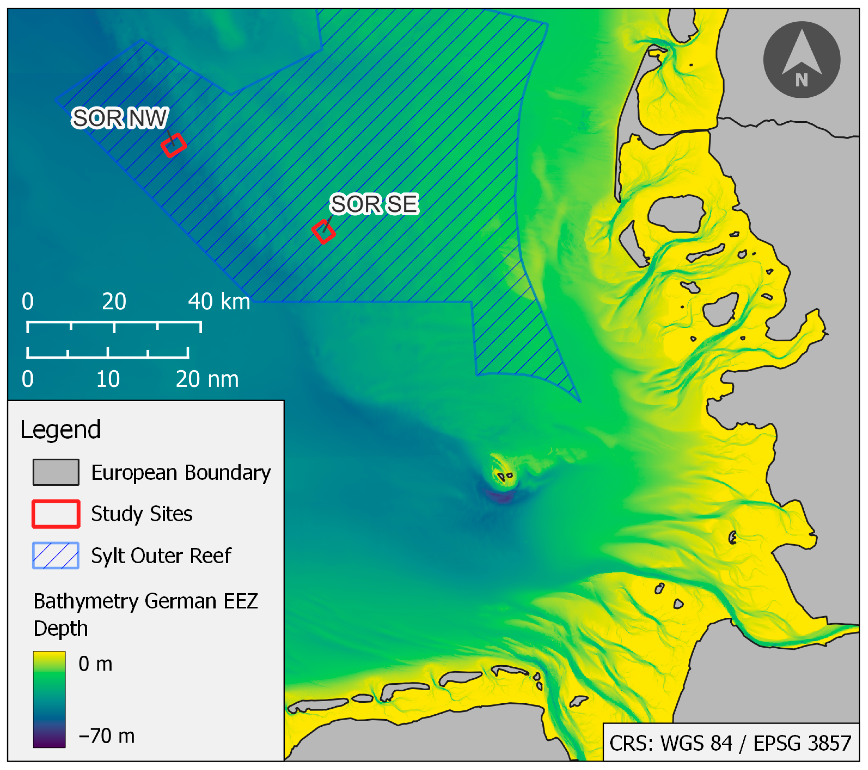
2. Geographical Setting and Study Sites

The algorithms were tested on datasets that were gathered during research cruises in 2022. The two study sites are situated within the MPA Sylt Outer Reef (SOR) in the German Bight—see Figure 1. The sites, based on their relative geographical location, further referred to as SOR NW and SOR SE, have been chosen because they show a great variety of seafloor characteristics with frequent shifts in sediment compositions but also consist of areas with homogenous sediment distribution. With these properties, classifying the backscatter mosaics should pose a challenge to the algorithms and thus help to highlight the weaknesses and strengths of the different approaches more effectively. The sites include an area of 13.6 km² and 12.6 km² with an average depth of 45 m and 28 m, respectively.

The German Bight is part of the relatively shallow water body of the southern North Sea, with a mean water depth of around 30 m. The hydrodynamic regime is dominated by tidal currents, which are directed along the coast in a counter-clockwise direction and are driven by tidal residual circulation [11]. The currents are further enhanced by westerly and southwesterly winds [12]. Tidal dynamics, wave actions, wind-driven currents, and mixing determine seabed sediment dynamics. The recent state of the geomorphology and surface sediments of the Sylt Outer Reef is the result of several glacial advances and retreats during the Pleistocene. Surface sediments consist of heterogeneously distributed coarse-grained lag deposits, which are mainly composed of reworked siliciclastic moraine deposits. The dominant grain size of the reworked material varies from coarse sand to gravel, which is partly mixed with pebble- to boulder-sized particles. The coarse sediments are partly covered or surrounded by Holocene marine fine- to medium-grained sands [13]. Surficial finer sediments are deposited by a series of sedimentary infillings, which were driven by wind, waves, tides, and storm events during the Holocene Transgression [14].

Figure 1. The study sites in the Sylt Outer Reef located in the eastern part of the German EEZ North Sea; European boundary data from Ref. [15], Sylt Outer Reef coordinates from Ref. [16], and bathymetry background data from Ref. [17].

Figure 1. The study sites in the Sylt Outer Reef located in the eastern part of the German EEZ North Sea; European boundary data from Ref. [15], Sylt Outer Reef coordinates from Ref. [16], and bathymetry background data from Ref. [17].

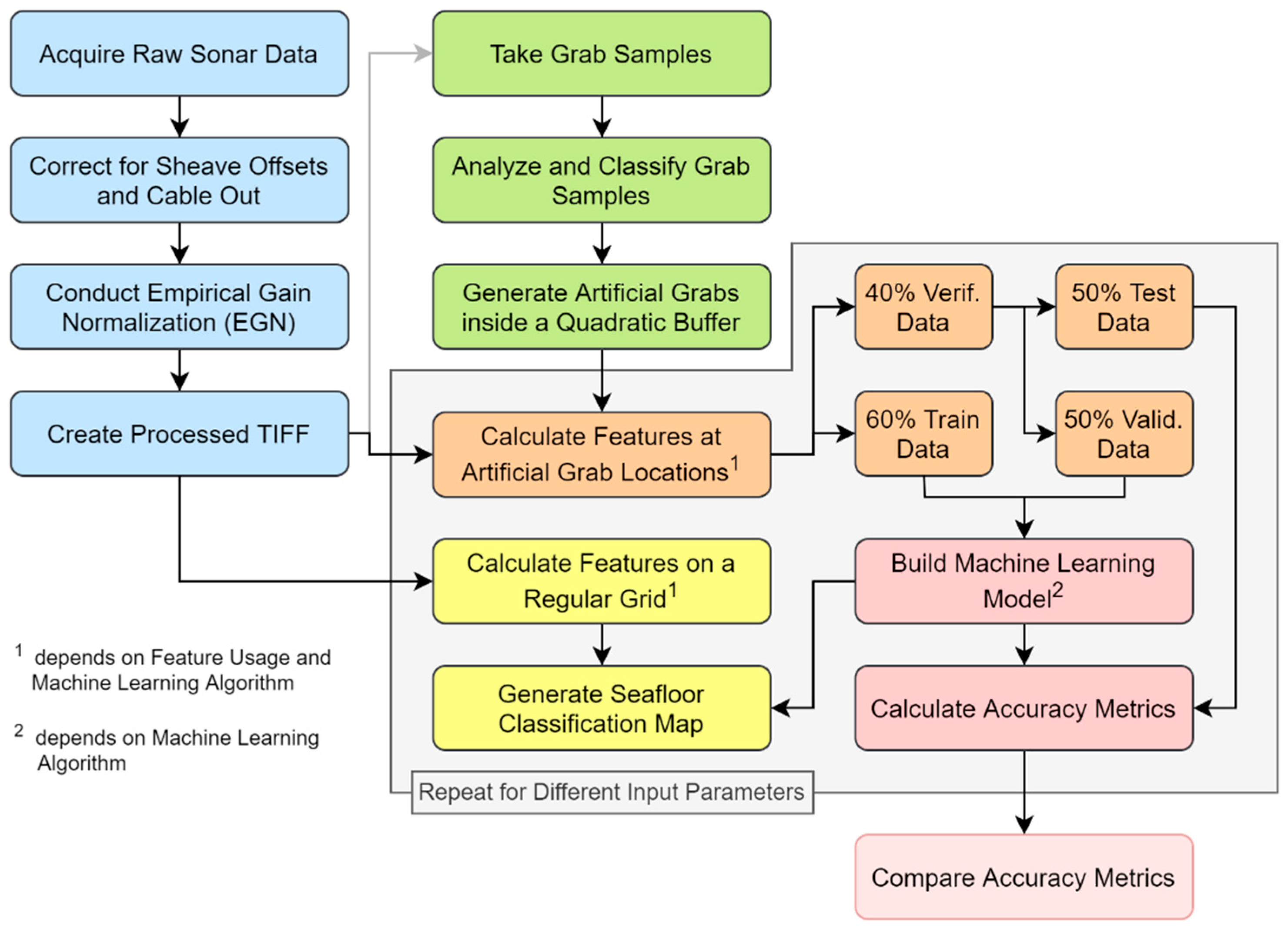
3. Material and Methods

The acoustic classification has been carried out based on hydroacoustic backscatter mosaics, which were generated using SSS (side-scan sonar) data. The backscatter information has been validated by ground-truthing taken by bottom-grab sampling. The amalgamation of both data sources is the basis for an interpreted classification with regards to the given geological/sedimentological background of the habitats.

Several processing steps are required to transform the raw SSS data and information from the grab samples into datasets that can be utilized for the training of machine-learning algorithms, ultimately allowing for the computation of a seafloor classification map. The required steps will be explained individually in the following Sections. A generalized flow chart of the overall process is shown in Figure 2.

3.1. Spatial Mapping with a SSS System

The SSS data were acquired in June 2022 during the survey HE602 on the RV Heincke [18] with an EdgeTech 4200 MP SSS system (EdgeTech, Boston, MA, USA). The technical specifications of the used system are shown in Table 1 The towed SSS dual-frequency system EdgeTech 4200 MP was operated with a swath of 200 m (>100% coverage of the area with a given profile distance of 75 m). During acquisition, a constant vessel speed of approximately 5 knots was targeted to ensure homogeneous along-track resolution. Moreover, the depth of the towfish was targeted to be at least half of the water depth to prevent direct wave reflections inside the seafloor backscatter data.

The sonar data were recorded with EdgeTech Discover 4200 [19] and processed with SonarWiz™ 7.09.02 [20]. The post-processing included the steps of (i) slant range correction, (ii) empirical gain normalization (EGN), and (iii) layback correction, as exemplarily described in Ref. [21]. The EGN tables were separately calculated for both study sites. In order to not blend any textures, the overlapping areas of individual profiles have not been combined but instead displayed on top of each other. In accordance with the BSH guideline for seafloor mapping in German marine waters [22], the data were exported as a mosaicked, georeferenced TIFF file with 8-bit quantization (256 grayscale values) in spatial resolutions of 5 m, 1 m, and 0.25 m for each of the recorded frequencies. However, in the following, only the mosaics with a resolution of 0.25 m and a frequency of 600 kHz are utilized for classification as they contain the most meaningful information about the surface of the seafloor. Low backscatter areas are represented by high gray values (about 55 to 254), while high backscatter intensity is characterized by low gray values (0 to about 54). The processed mosaics of the high-frequency SSS data are shown in Figure 3.

Table 1. Technical specifications of the EdgeTech 4200 MP SSS system [23].

System	Frequencies	Horizontal Beam Width	Vertical Beam Width	Across-Track Resolution	File Formats
EdgeTech 4200 MP	300 kHz	0.54°	50°	3 cm	.jsf, .xtf
	600 kHz	0.34°		1.5 cm

Table 1. Technical specifications of the EdgeTech 4200 MP SSS system [23].

System	Frequencies	Horizontal Beam Width	Vertical Beam Width	Across-Track Resolution	File Formats
EdgeTech 4200 MP	300 kHz	0.54°	50°	3 cm	.jsf, .xtf
	600 kHz	0.34°		1.5 cm

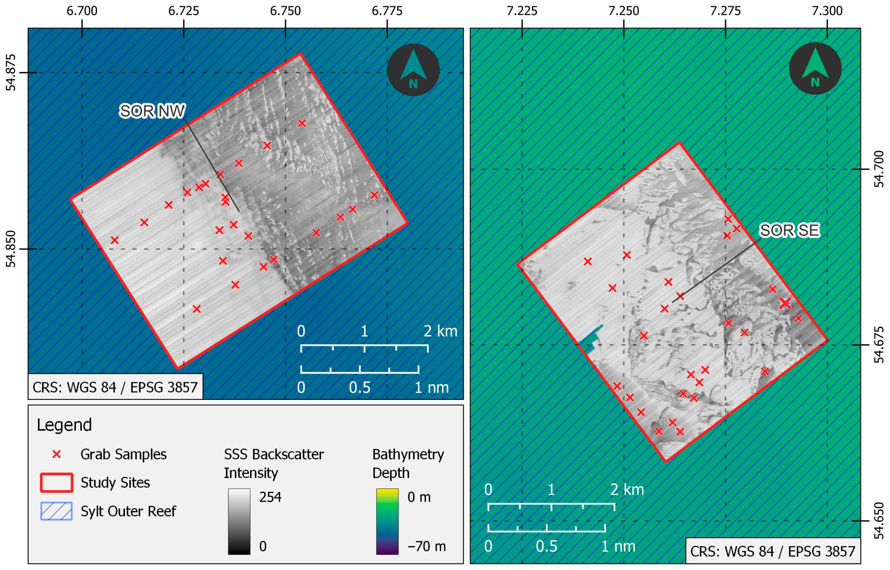
3.2. Ground-Truth Data from Grab Samples

Ground-truth data are crucial for the classification of non-invasively acquired data as it provides directly measured properties of the environment. The information about the seafloor characteristics obtained at given locations with a sediment grab sampler can be used by humans as well as machine-learning algorithms to learn about the relationships between the acoustic image data and the underlying real-world seafloor composition.

The ground-truth data for the two study sites were obtained with a shipek grab sampler during cruise SE2233 with the RV Senckenberg in August 2022. While ideally sampling and mapping should be done simultaneously to ensure optimal correlation, the given time span between mapping and sampling was about two months, which is not ideal but acceptable for the less dynamic environment of the study areas. The sample locations have been chosen based on different visible textures (i.e., seafloor surface characteristics) from the mosaicked SSS data at the study sites SOR SE and SOR NW. Each distinct texture was sampled between three and six times in different locations, with the aim of maximizing the distance between a given sample location and any visual changes in surrounding backscatter patterns. The sediment samples were photographed, examined, and documented on site; a small portion of the grab content was collected, later analyzed via ¼ phi sieving in the lab, and finally processed in GRADISTAT [24]. Whenever two grab samples appeared to be close to identical on site, due to limited capacities, only one of the samples was analyzed in the lab. The characteristics of the analyzed sample were then transferred to the related sample. After analyzing the samples, they were manually classified based on the grab sample surface (i.e., the photos) and the grain size distribution. The identified classes were very fine (i.e., silty/muddy), fine (i.e., fine sand), medium fine (i.e., medium sand), coarse (i.e., coarse sand/fine gravel), and very coarse (i.e., gravel), as well as two mixed classes: Fine with coarse side components and coarse with very coarse side components. Twenty-three samples were processed for the study site SOR NW and 27 for the study site SOR SE. The locations of the grab samples can be found in Figure 3.

3.3. Quantization Level and Size of the Image Patches for the Classification

In order to predict seafloor surface characteristics based on their backscatter intensity (i.e., grayscale values) in SSS mosaics, it is necessary to analyze the areal properties and patterns of the grayscale values that are present at a desired location (e.g., see Ref. [25]). Therefore, image patches are extracted from the mosaic at the sampling locations, which establishes a direct link between the seafloor observed in the grab sample and the texture visible in the mosaic and hence enables machine-learning algorithms to learn relationships between the data types.

In general, the quantization (i.e., the number of grayscale values) and the size of these image patches are arbitrary. However, for the given task of predicting seafloor characteristics, there are practical limits on how to choose these parameters. A high number of grayscale values preserve a large amount of information but might also contain noise, whereas a smaller number of grayscale values minimizes leftover noise in the data but reduces the available information. Larger patch sizes allow for greater generalization but are prone to representing mixed textures of different underlying classes. Smaller patch sizes have a higher chance of solely containing data that represents a unique seafloor component, but simultaneously might also only contain a fraction of the information needed to correctly approximate the underlying seafloor structure. Moreover, computation performance plays a role, as large image patches and many grayscale values are generally more computationally expensive to produce.

In order to find a suitable image patch size and the number of grayscale values for the classification of SSS data acquired in the Sylt Outer Reef, we tested image patch sizes of 32 px, 16 px, and 8 px (8 m, 4 m, and 2 m per image patch with the given spatial resolution of 0.25 m per pixel) as well as 8-bit quantization (256 grayscale values) and 6-bit quantization (64 grayscale values).

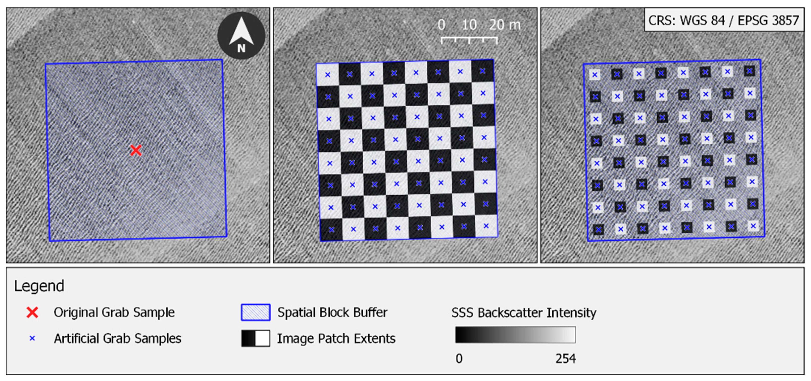
3.4. Generating Training, Test and Validation Data from Sample Locations

Most machine-learning algorithms and performance estimation methods rely on splitting the available ground-truth information into subsets of training, test, and validation data. While training data are used to build the prediction model itself, validation data are used to tune model parameters [26] and prevent overfitting [27]. After the prediction model has been built, its performance will be evaluated using the test data.

Due to the high amount of work and time that goes into gathering and analyzing grab samples, the available dataset for the given task of seafloor classification is usually very small. As machine-learning algorithms are dependent on large and representative datasets, this circumstance poses a great challenge.

Fortunately, there are multiple approaches to increase the number of data points for the training and testing of machine-learning algorithms. An often-used method to generate data is data augmentation, in which the extracted image patches are randomly rotated, translated, mirrored, sheared, or radiometrically altered [28]. A very recent method is the use of generative adversarial networks (GAN), as conducted in Ref. [29], in which two communicating artificial neural networks synthesize new image patches based on a given, smaller dataset. However, both of these methods rely on the transformation of a given input and thus do not create new, independent data.

Instead of artificially generating image patches, the authors in Ref. [2] artificially generated new grab sample locations. They assume that inside a manually specified area around the original location of a given grab sample, the seafloor is made of the same components as the actual sampling locations (see Figure 4, left). Inside that area, image patches can be extracted from the mosaic and treated as a fictional grab sample with the same properties as the actual grab sample. Even though this approach is dependent on assumptions, we chose this technique to increase the number of data points as the created data itself is not artificially generated.

After specifying the complete dataset, the available image patches must be split into train, test, and validation datasets. In order to minimize correlation within the training and test/validation data, the image patches are spatially blocked [30] in a chessboard pattern, where either “white” or “black” patches will be used as training and the other color as test/validation data (see Figure 4, middle). As this would result in a 50/50 split, random image patches from the test/validation dataset (e.g., “black patches”) are transferred to the training dataset (e.g., “white patches”) until the desired split of 60% training data is reached. The remaining non-training patches are then equally split into 20% validation and 20% test data. Patches from within the validation and test datasets (e.g., “black patches”) are guaranteed not to share any borders with each other. Thus, the possibility of underestimating prediction errors due to spatial autocorrelation is minimized [30]. The process of assigning the datasets is repeated ten times with random splitting and random color assignment (e.g., “white patches” as training data and “black patches” as test/validation data, and vice versa) for every classification. For each split, a prediction model is computed. The estimated performance of the model is then calculated by averaging the performance metrics achieved by classifying the test data. The underlying splitting technique of randomly assigning data points to training, test, and validation datasets without replacement during multiple runs is called Monte-Carlo cross-validation (MCCV) [31,32].

It should be noted that the number of data points created this way depends on the chosen size of the image patches. To ensure that the results are comparable, the locations of artificially created grab samples are the same for every computation and therefore determined by the largest image patch size (i.e., 32 px; see Figure 4, right).

3.5. Machine-Learning Algorithms

Prediction maps of the seafloor surface characteristics in the study sites were computed with three different supervised machine-learning algorithms: Support vector machines with a linear kernel (SVM-L) (e.g., [33,34]), random forests (RF) (e.g., [2,4,5,9,10,35,36,37]), and convolutional neural networks (CNN) (e.g., [1,38,39,40]). SVMs have been widely used in remote sensing (see [41] for a detailed review) and seafloor classification tasks. They aim to find hyperplanes in feature space that result in an optimal separation of the classes given in the dataset. By using the SVM with a linear kernel, linear separability of the dataset is assumed [42]. Non-linear data can be separated by mapping the data to a higher-dimensional feature space (e.g., with a polynomial or radial basis function (RBF) kernel). Nevertheless, we opted for the use of a linear kernel since, on the one hand, the comparison of multiple kernels would make this comparative study too extensive, and, on the other hand, RFs and CNNs are already non-linear classifiers. Thus, a linear kernel provides valuable information regarding the linear separability of the present data. Besides the kernel, the regularization parameter C is an important hyperparameter of SVMs [43]. In test runs, nearly identical prediction models were observed for parameter values between 0.1 and 100. As a result, we opted for a value of C equal to 1. Additional information on SVMs and kernel-based learning can be obtained from [42,43].

RFs are an ensemble of multiple decision tree classifiers (DTCs). A single decision tree classifies a dataset by recursively splitting it into smaller subsets based on a feature-driven decision that leads to the highest separation between the subsets. The quality of separation is evaluated by a splitting criterion (i.e., subset homogeneity) [44]; for our computations, we used the Gini impurity. By generating multiple DTCs with randomly selected sub-training sets from the original dataset, a robust RF ensemble is created in which the most frequent class prediction of the DTCs will be considered the RF’s prediction [45]. In accordance with the findings in Ref. [46], we utilized 100 individual classifier trees per RF ensemble. To avoid overfitting due to overly complex (i.e., deep) decision trees, the maximum depth of the trees is determined using the validation data. The increase in classification accuracy with increasing tree depth was approximated with a logistic function. As soon as a given depth reaches the function’s supremum, that depth is chosen as the maximum tree depth for the RF. For more information regarding RFs, see Ref. [45].

The number of features used in both SVM-L and RF is dependent on the results of the feature extraction and feature selection algorithms, which will be explained in Section 3.6. For the implementation of SVM-L and RF, the Python library Scikit-learn was used [47]. Hyperparameters that have not been explicitly mentioned were kept at their default values provided by the Scikit-learn library.

RF and SVM-L are referred to as traditional machine-learning techniques, as these algorithms require feature calculation and, if necessary, preprocessing, feature extraction, and feature selection. Deep learning algorithms, on the other hand, are able to generate a prediction model directly from the input data (e.g., images) without the necessity of feature calculation [48]. For additional information on deep learning algorithms in general and CNNs in particular, please refer to studies such as Ref. [48] or [49].

In the context of SSS imagery, deep learning has been utilized for classification, segmentation, and object detection. A comprehensive study on the usage of deep learning methods for a variety of tasks regarding the analysis of sonar imagery can be found in Ref. [50]. For classification tasks, the go-to deep learning technique used in recent literature is the convolutional neural network (CNN). Multiple, complex CNNs with millions of parameters, which were originally designed to perform well on the ImageNet dataset [51], have been used for seafloor classification in previous papers (e.g., GoogLeNet in [38] and VGG-16, ResNet, DenseNet, and others in [40]). However, Ref. [39] showed that for small datasets (<700 data points), a shallow CNN with two convolutional layers performs better than a deep CNN with five convolutional layers.

Based on these findings, we implemented the shallow CNN architecture with two convolutional layers presented in Ref. [39] with some minor modifications. The adopted architecture consists of 32 kernels (i.e., neurons) in the first convolutional layer and 64 kernels in the second convolutional layer, both of which use the ReLu (rectified linear unit) activation function. The kernel size is set to 3 × 3 px and the pooled area to 2 × 2 px. Instead of 1024 units in the penultimate dense layer (or fully connected layer), we chose to use 64 units, which proved to deliver comparable results with a fraction of the computation time. The last layer activation function was set to the softmax function, as it is commonly applied for multiclass single-label classification [49]. To prevent overfitting, we further added a batch normalization layer [52] as well as dropout regularization [53]. According to Ref. [54], batch normalization and dropout regularization should not be applied directly one after the other. To avoid a drop in model performance, we implemented the batch normalization after the first convolution operation and the dropout regularization after the first dense layer with a dropout of 20%, as recommended in Ref. [54]. RMSprop, developed in Ref. [55], was chosen as the optimization function for stochastic gradient descent. As a multiclass classification task is given, categorical cross-entropy is used as the loss function.

Finally, we utilized the early stopping technique (see Ref. [56]), in which the training of the CNN is aborted as soon as the validation loss stops increasing for ten consecutive training epochs. The learning rate has been set manually in order to ensure a satisfactory learning process without fluctuations. The deep learning algorithms have been implemented in Python with the Keras software library [57]. Again, default hyperparameters were applied when not specifically stated otherwise, as tuning hyperparameters based on small datasets could lead to the prediction model not being independent of the test data, which could bias the model’s performance.

3.6. Input Data and Input Data Processing

As mentioned, traditional machine-learning algorithms such as SVMs and RFs rely on features as input data. The features are derived from the image patches extracted from the processed SSS mosaics (see Figure 3). We tested three different types of feature groups for their ability to discriminate the seafloor classes present in the Sylt Outer Reef: aggregation functions, textural features from gray-level co-occurrence matrices, and Weyl coefficients.

A straightforward method of image patch analysis is the use of aggregation functions (hereafter abbreviated as AGG), which return simple statistical values. We include the minimum and maximum gray values, and the mode, mean, and variance of the gray values in that feature group.

The downside of aggregation functions is that they do not describe the pattern of image patches. Therefore, a more sophisticated approach to describing image patches is the gray-level co-occurrence matrices (GLCM) proposed in Ref. [58]. GLCM textural features have been widely used for seafloor classification and habitat mapping and have been proven to be suitable for sonar imagery classification (e.g., see Refs. [34,59,60,61]). In a GLCM, the distribution of co-occurring gray values in the image patch is stored for a given interpixel distance (i.e., a spatial component) and a given calculation angle. That matrix is then used to derive multiple features to describe the texture of the image patch [58]. According to Ref. [62], broadly used GLCM features are angular second moment, contrast, correlation, dissimilarity, entropy, and homogeneity, as well as mean and variance (not to be confused with mean and variance values of the aggregation functions). These features correlate with the features used in the papers mentioned above, which is why we included these eight features in our computations. In accordance with the findings of Ref. [9], we chose interpixel distances of 5 px and 10 px and averaged the textural feature values for the four available directions of 0°, 45°, 90°, and 135°.

A relatively new approach to describing the texture of image patches with Weyl coefficients was introduced in Ref. [63] and successfully adapted for seafloor classification data in Ref. [2]. The Weyl coefficients result from the so-called Weyl transform (WT), for which the covariance matrix of the given image patch and the multiscale signed permutation matrices from the binary Heisenberg–Weyl group are utilized. As the number of coefficients grows by n⁴ (where n is the size of the image patch), the calculation of Weyl coefficients is only suitable for very small image patches. For this reason, Ref. [63] split larger image patches into 4 × 4 px sub-patches and aggregated their absolute coefficient values per sub-patch. With this technique, 256 Weyl coefficients were calculated for each image patch, regardless of their size. A detailed mathematical description of the calculation steps can be found in Refs. [2,63].

The features of the three feature groups (AGG, GLCM textural features, and Weyl coefficients) were either combined into a single classification or used separately in order to evaluate their impact on the classification result. To account for different scales of and correlations between features, all used features are normalized with min–max feature scaling and then transformed into uncorrelated principal components (PCs) using a PCA [64] (feature extraction). As suggested in Ref. [64], the PCs with the greatest explained variance were retained until their cumulative contribution reached 90% of the total variance present in the dataset. In the last step, recursive feature elimination (RFE; [65]) is used so that only those features are kept for classification with the traditional machine-learning algorithms that contribute to the given task (feature selection).

While CNNs do not need input features and can be trained solely with image patches, the possibility of using Weyl coefficients for CNNs is described in Ref. [66]. The authors proposed to use the symmetrical and skew-symmetrical matrix of the image patch (instead of its covariance matrix) to calculate the Weyl coefficients. The patch Weyl transform (PWT) generates as many coefficients as there are gray values in the image patch (n × n) and can thus be interpreted as an image patch itself. The resulting PWT patches for the symmetrical and skew-symmetrical matrices of the SSS image patch were therefore used as additional color channels of the image patch and then fed into the CNN.

4. Experimental Results

Although the two study sites in the Sylt Outer Reef are comparably heterogenous with frequent shifts in the seafloor sediment composition, the area size of assumed homogeneity was set to 64 × 64 m² with the original grab sample in the center. Assuming homogeneity over such an area was made possible by specifically choosing sampling locations with a preferably large distance to visual changes in the pattern of the backscatter mosaic. With the resulting two-sided buffer of 32 m and the maximum image patch size of 32 × 32 px (which is equivalent to 8 × 8 m for a 0.25 m resolution of the backscatter mosaic), 64 artificial grab sample locations were generated for every original grab sample (see Figure 4). This results in a total of 1536 data points for the study site SOR NW and 1728 data points for the study site SOR SE. The distribution of the classes in the datasets can be seen in Figure 5. From these 64 artificial locations per sample, 60% (38) were assigned to the training and 20% (13) to the test and validation datasets. The datasets were generated using the splitting technique described in Section 3.4 to minimize spatial correlation within the validation and test data. As mentioned, the training process of the models was repeated ten times with different compositions of training, test, and validation datasets.

For each of the data points, the features required for the model training and evaluation of the prediction model are calculated based on the underlying backscatter intensities.

Table 2. Approximate number of data points for which all required features can be calculated within one second; used system: Intel^® Core™ i5-1135G7 @ 2.40 GHz, 8 GB RAM, Intel^® Iris^® Xe Graphics (Intel, Santa Clara, CA, USA).

	Used Features	32 px		16 px		8 px
		8-bit	6-bit	8-bit	6-bit	8-bit	6-bit
SVM-L and RF	All	8	12	15	45	20	114
	AGG	1389	1316	1493	1453	1429	1431
	GLCM	17	303	22	327	21	322
	WT	13	12	50	52	168	172
CNN	All	13	12	309	304	1190	1272
	Gray *	-	-	-	-	-	-
	PWT	13	12	309	304	1190	1272

* Using only gray scale image patches requires no additional computation time.

shows the number of data points for which the features can be calculated within a time span of one second.

To address the present class imbalance, the class weights during training have been adjusted inversely proportional to the class frequencies during training of the models. Additionally, the Matthews correlation coefficient (MCC; [67]) was calculated from the model’s performance on the test data. The MCC is a useful metric when dealing with unbalanced data and serves as a more reliable performance measure than Cohen’s kappa, according to Ref. [68]. An MCC close to 1 indicates a very good classification model, whereas a model with an MCC of 0 performs as well as classification with random chance. Negative values imply a negative correlation between the model and prediction [69]. The MCC values scored with the tested machine algorithms using different input data can be found in

Table 3. Mean MCC values from ten runs for different classification algorithms in the study site SOR NW; highest and lowest MCC for varying image patch sizes and number of grayscale values are denoted in bold and italic, respectively; highest MCC for a given machine-learning algorithm is denoted with an underline; highest overall MCC is denoted with a star.

	Used Features	32 px		16 px		8 px
		8-bit	6-bit	8-bit	6-bit	8-bit	6-bit
SVM-L	All	0.49	0.50	0.44	0.45	0.36	0.36
	AGG	0.38	0.37	0.37	0.38	0.37	0.38
	GLCM	0.52	0.52	0.46	0.47	0.39	0.37
	WT	0.22	0.21	0.12	0.13	0.05	0.05
RF	All	0.57 *	0.55	0.42	0.47	0.39	0.38
	AGG	0.43	0.43	0.39	0.42	0.39	0.39
	GLCM	0.57 *	0.57 *	0.49	0.48	0.37	0.38
	WT	0.27	0.26	0.12	0.10	0.05	0.03
CNN	All	0.41	0.42	0.38	0.37	0.33	0.31
	Gray	0.43	0.44	0.39	0.40	0.37	0.37
	PWT	0.18	0.24	0.06	0.09	0.06	0.03

and

Table 4. Mean MCC values from ten runs for different classification algorithms in the study site SOR SE; highest and lowest MCC for varying image patch sizes and number of grayscale values are denoted in bold and italic, respectively; highest MCC for a given machine-learning algorithm is denoted with an underline; highest overall MCC is denoted with a star.

	Used Features	32 px		16 px		8 px
		8-bit	6-bit	8-bit	6-bit	8-bit	6-bit
SVM-L	All	0.82	0.82	0.75	0.75	0.66	0.67
	AGG	0.70	0.70	0.69	0.69	0.62	0.62
	GLCM	0.62	0.65	0.62	0.65	0.62	0.61
	WT	0.55	0.55	0.41	0.41	0.27	0.27
RF	All	0.85	0.87 *	0.80	0.79	0.62	0.65
	AGG	0.73	0.73	0.71	0.70	0.67	0.67
	GLCM	0.75	0.76	0.67	0.70	0.65	0.64
	WT	0.65	0.61	0.48	0.45	0.29	0.31
CNN	All	0.73	0.73	0.65	0.66	0.60	0.59
	Gray	0.85	0.85	0.79	0.79	0.71	0.70
	PWT	0.42	0.52	0.26	0.38	0.17	0.24

for the study sites SOR NW and SOR SE, respectively.

4.1. Impact of the Quantization Level and Image Patch Size

Based on the MCC values shown in Table 3 and Table 4, the tested levels of quantization appear to have little to no effect on the model’s performance. Across the image patch sizes, machine-learning algorithms, and study sites, the MCC values are mostly constant for 6- and 8-bit quantization. Only when the image patches derived from the PWT coefficients are exclusively used in the CNN, the model performance seems to be positively impacted by a reduced number of grayscale values of 64.

Conversely, the image patch size exerts a great influence on the numerical performance across all of the algorithms. In general, the MCC values tend to decrease with a decreasing image patch size. This observation is especially true when classifying the data based on the coefficients of the Weyl transform. While for the AGG and GLCM features, the MCC values are only slightly decreasing with smaller image patch sizes, the MCC values for the Weyl coefficients of the 32 px image patches are about twice as high as for the 8 px image patches.

These observations are also reflected when visualizing the principal components (PCs) derived from all available features (i.e., five AGG features, 16 GLCM textural features, and 256 Weyl coefficients). Figure 6 shows the boxplots of the two PCs with the highest feature importance for different levels of quantization and image patch sizes. When comparing the PCs derived from an image patch of 32 px size and 8-bit quantization (Figure 6a,b) with those of a 6-bit quantization (Figure 6c,d), the distribution of the data points seems close to identical. On the other hand, the effects of reducing the image patch size from 32 px to 8 px (Figure 6e,f) are observable. Finer sediment compositions show an increased dispersion with reduced patch size for the PC with the highest feature importance (Figure 6a,c,e). Although the dispersion of data points from coarser sediment classes is partially reduced compared to those of larger image patches of 32 px, the heterogeneity between all sediment classes has decreased, which hinders the separation of the classes by the machine-learning algorithms. The same applies when looking at the PC with the second highest feature importance (Figure 6b,d,f).

Unfortunately, as the CNN relies on the image patches themselves rather than on derived features, there is no intuitive way of visualizing the data points in a feature space for further evaluation. Nonetheless, the MCC values decrease in a similar way for the CNN as for the traditional machine-learning algorithms, which suggests that the neural network is subject to similar limitations at smaller image patch sizes as the other methods.

Although it does not affect the overall model performance, 6-bit quantization of the image patches led to a 15-fold increase in the number of GLCM features that can be calculated in a given period of time compared to 8-bit quantization, as can be seen in Table 2. As expected, due to their mathematical foundation, the other features’ computation times are not affected by the number of gray values. The size of the image patches has a particularly strong impact on the computation time of the Weyl coefficients since the number of coefficients depends on the number of pixels contained in the image.

4.2. Impact of the Machine-Learning Algorithm and Input Data

The overall best numerical model performance in both study sites has been achieved with the RF algorithm, with an MCC of 0.88 in the study site SOR SE and 0.57 in SOR NW. Compared to the other algorithms, the RFs reliably produce the best prediction models independent of the input features used for classification. When using the most suitable image patch size of 32 px, the MCC scores of the SVM-L models are outperformed by the RF models by about 0.05 on average in each of the study sites. The MCC of the SVM-L model most likely suffers from its assumption of linear separability of the dataset, as the scatterplots from Figure 7 suggest some non-linearity, especially for the coarser sediment components.

However, both traditional machine algorithms show an improved performance by combining all feature groups (AGG, GLCM, and WT) compared to using just a single feature group. Through the use of combined features, the MCC for classification of 32 × 32 px image patches in the study site SOR SE was—on average—improved by 0.14 and 0.15, respectively, compared to classifying solely with AGG features (average MCC of 0.71) or GLCM textural features (average MCC of 0.70). In the study site SOR NW, the combination of the feature groups also leads to an apparent boost in model performance, although the overall model performance is not as good as in the other study site. With combined feature groups, the average MCC value is 0.53 and therefore increased by 0.13 or 0.10 compared to solely using the feature groups AGG or GLCM. Although the WT coefficients yield satisfactory results in the study site SOR SE with a maximum MCC of 0.65, the WT coefficients are constantly outperformed by the other feature groups by margins ranging from 0.06 to 0.36. The same observation can be made for the study site SOR NW. Nevertheless, the good results of combining the features indicate that the WT coefficients contribute some additional information about the seafloor that is not covered by the other feature groups.

The CNN performs very well on the dataset from study site SOR SE with a maximum MCC of 0.85, which is slightly better than the SVM-L model (0.82) and slightly worse than the RF model (0.87). However, the best numerical performance of the CNN in the study site SOR NW with an MCC of 0.44, is the worst of all tested algorithms by a margin of 0.08. Moreover, unlike the traditional machine-learning algorithms, the numerical performance of the CNN is not positively affected by the introduction of image patches derived from the PWT. Across all computations, only using the original grayscale image patches as training data for the CNN leads to the highest MCC values.

In terms of computation time, the traditional machine-learning algorithms perform best regarding the training of the model. For RF and SVM, on average, one iteration of model training took between one and six seconds, depending on the number of input features but regardless of the quantization level and image patch size. On the other hand, training a CNN prediction model took between 70 and 180 s with the given hyperparameters. However, it should be noted that computation time for the training of neural networks could be dramatically improved by using a GPU.

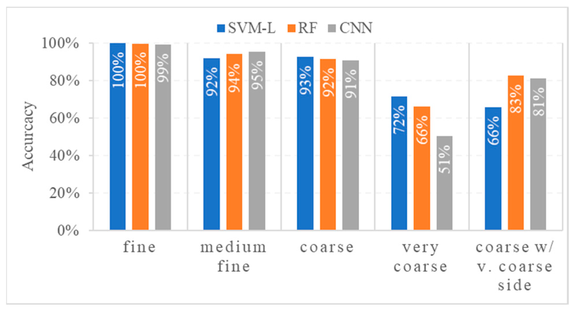
4.3. Model Performances on Different Seafloor Sediment Classes

Figure 8 and Figure 9 show the per-class accuracy reached for each machine-learning algorithm with an image patch size of 32 × 32 px and a radiometric resolution of 64 grayscale values for the study sites SOR NW and SOR SE, respectively. Although, in detail, the per-class performance varies from algorithm to algorithm, there are a few general observations that can be made: While all algorithms are capable of distinguishing between fundamental seafloor surface characteristics (e.g., fine, medium fine, and coarse) with high accuracies of 80% up to more than 95%, they fail to accurately predict mixed sediment components (i.e., classes fine with coarse side components and coarse with very coarse side components) as well as differentiating between similar classes (fine/very fine and coarse/very coarse). The comparatively poor results for the affected classes might be an indication that the given classes cannot be resolved with standalone SSS data and that some simplification is required. For example, mixed classes with side components could be discarded and instead merged into the class of their main or side component.

However, of all the algorithms tested, RF was the most likely to correctly assign even the problematic classes mentioned above, which presumably led to the superior MCC values shown in Table 3 and Table 4.

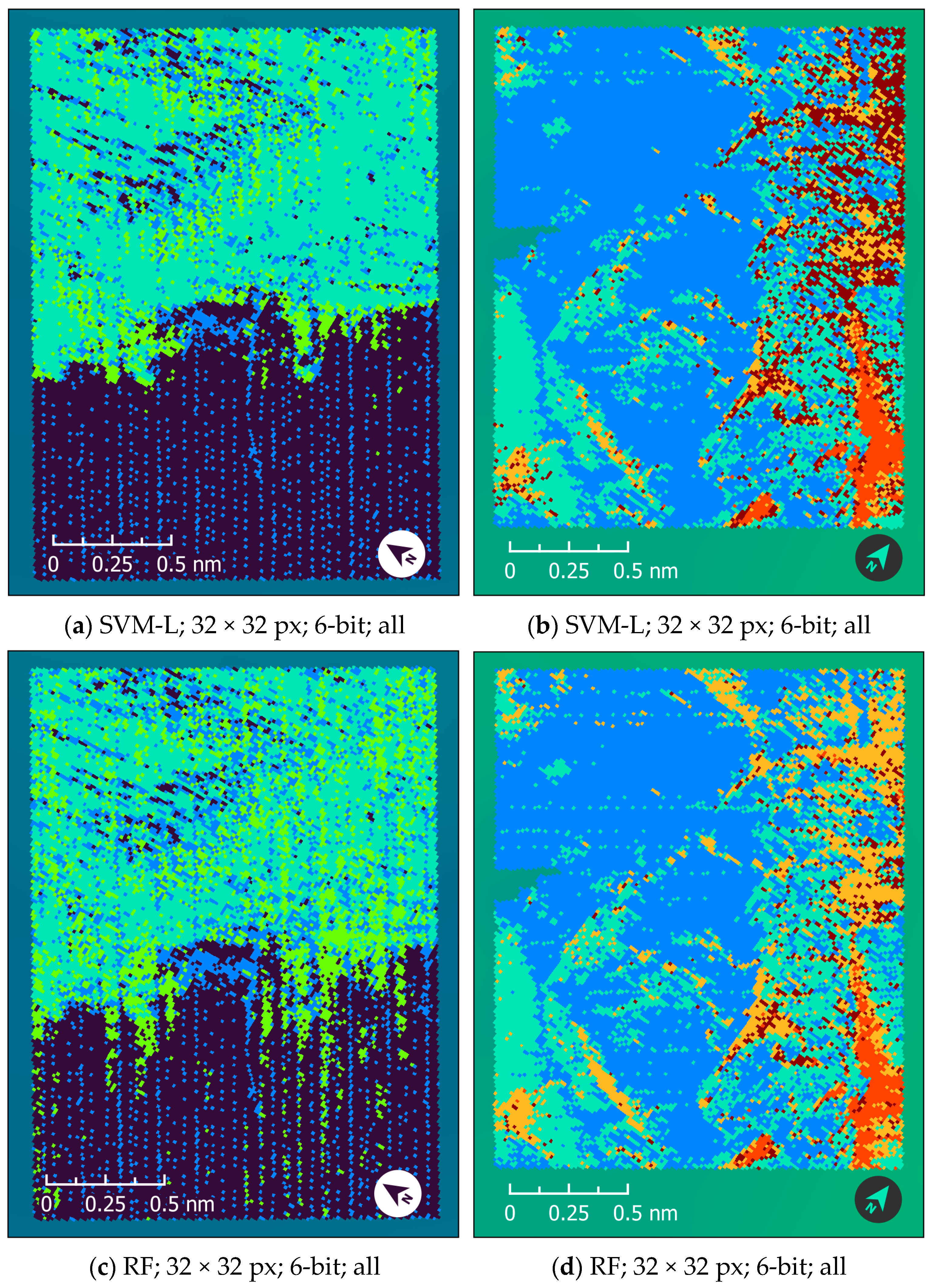
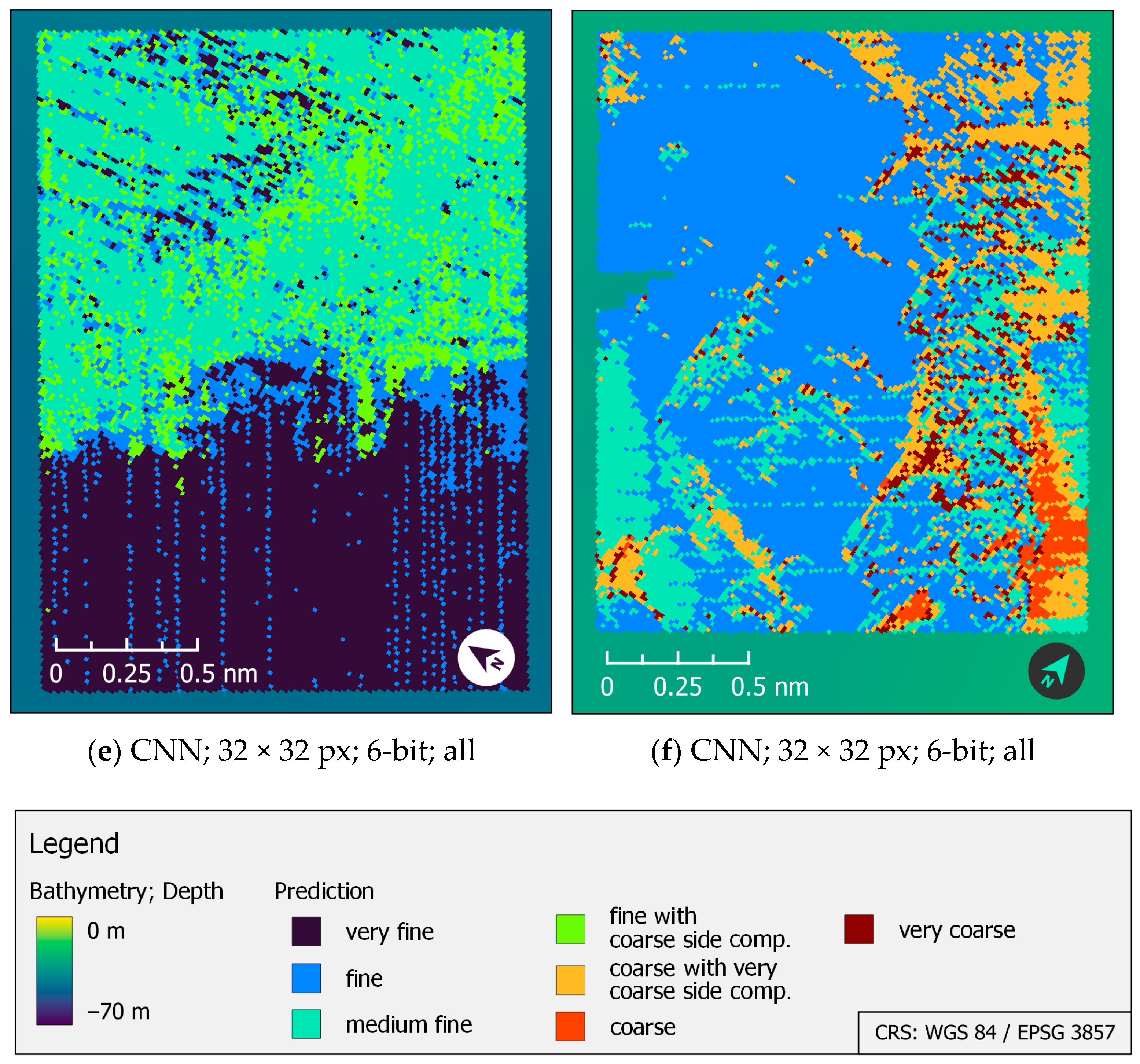
4.4. Visual Assessment of the Classification Maps

A purely numerical assessment of the classification results is problematic since it only includes the specific locations of the grab samples rather than the entire area of the study site. We, therefore, calculated classification maps for the depicted algorithms on a regular 25 × 25 m grid, which approximately led to 22,000 predictions (i.e., pixels) for the study site SOR NW and 20,000 predictions for the study site SOR SE. The predicted class corresponds to the most frequent prediction from the ten runs with random training, test, and validation datasets. The prediction maps are shown in Figure 10a–f.

Upon examination of the prediction maps in Figure 10a–f, the general appearance of the classification maps is quite similar for all algorithms. However, the maps still differ in detail. In study site SOR NW (see Figure 10a,c,e), there is a strong striped pattern, particularly in the southwestern half that results from the transition zone between individual SSS profiles. These stripes are especially pronounced in the prediction maps generated with traditional machine-learning algorithms. The northeastern half of the area has been comparably well classified by both the SVM-L and the CNN, while for the RF algorithm, the predictions of the classes fine and fine with coarse side components change with high frequency and without any visible underlying structure. The transition area between the finer and coarser sediment components is visually best approached by the SVM-L and CNN. When looking at the prediction maps and the numerical performance metrics from Table 3 and Table 4, the low accuracy in study site SOR NW most likely arises from this very transition zone between coarser and finer sediments and the high frequency of heterogeneity present in the northeastern part of the study site.

In the study area SOR SE (see Figure 10b,d,f), the transition between profiles is most noticeable in the prediction map calculated with the RF algorithm. For classification using SVM-L, a problematic zone lies in the northeastern part of the study area. There, the predictions of the classes coarse and coarse with very coarse side components are strongly mixed, resulting in a noisy classification. Contrary to the impression of the numerical performance of the algorithms, the overall most satisfactory classification maps are therefore generated by the CNN. Its prediction maps most closely match the visual appearance of the processed sonar mosaics. Although numerically beating the other algorithms, the maps derived from RF show more noise and are prone to misclassifications due to the transitions between individual profiles, which could indicate a possible overfitting of the training data. While presumably due to its linear data separation, the MCC scores and per-class accuracy for the SVM-L are comparably low, the classification maps themselves exhibit a smaller amount of noise compared to those of the RFs for this very reason. This highlights the importance of an area-based assessment of the results rather than purely relying on numerical performance metrics.

5. Discussion

As other papers suggested (e.g., Refs. [2,61]), we showed that a comparably bigger patch size of 32 px results in higher accuracies compared to smaller patch sizes. The better performance of larger image patches may be explained by the presence of noise, artifacts (e.g., stripe noise or signals from the water column), and non-sediment-related components (e.g., stones) in the backscatter data. The smaller the image patches, the greater the influence of those patterns on the performance of the algorithms. Whether even larger image patches of 64 px or 128 px further improve the results could be part of future studies.

In terms of the number of grayscale values depicted per image patch, several studies have found that GLCM textural features provide a high predictive value starting from 32 grayscale values (i.e., 5-bit quantization) [9,59,70]. We not only verified that observation for 64 grayscale values (6-bit quantization) but further extended it to the use of Weyl coefficients derived from both the WT and the PWT. Although we were not able to reproduce the findings in Ref. [2], who showed a superior performance of WT-derived coefficients over GLCM textural features, our results do indicate that these coefficients provide additional information about the seafloor that can be utilized by machine-learning algorithms and improve the performance of the models. Unfortunately, this cannot be said about the PWT-derived coefficients used in CNNs, as they did not lead to any improvements and even worsened the classification results. Our assumption is that of all the Weyl coefficients, only a few have sufficient descriptive power regarding the classification task. While we utilized feature elimination and extraction to remove less informative variables for the traditional machine-learning algorithms, the CNN has to deal with all coefficients at once and thus might not be able to extract meaningful information.

For our tested data, the machine-learning algorithms used produced comparable results, with slight advantages for CNNs over traditional machine-learning methods. Despite the RF achieving the highest MCC scores of all algorithms tested, in broad transition zones where the sediments show a lateral trend of grain size shift in the particle composition (as can be seen in study site SOR NW), the RF was visually outperformed by both SVM-L and CNN. The same applies to areas where there is stripe noise and differences in contrast between individual SSS profiles. This indicates a possible overfitting of the prediction maps generated by the RF algorithm.

However, all of the tested algorithms have limitations in correctly classifying areas at the edges of the SSS profiles and smooth sediment transitions. The first of which introduces contrast changes in areas of identical sediment components, while the second of which is challenging because the algorithm is confronted with patterns that are not present in the training data (i.e., superimposed sediment components). Next to being a challenging region, transition zones pose a threat to the assumption of homogeneity around the grab location that was introduced in Section 4. Even for the human eye, changes in sediment composition are difficult to spot in areas of gradually shifting sediments. To counteract the limitations mentioned, it might be necessary to either reduce the number of classes or increase the number of grab samples. A third option could be to reduce the area of assumed homogeneity whenever the grab sample lies within a transition zone or a comparably challenging area. This, however, comes at the cost of losing training data and should be carefully considered. Additionally, filtering the mosaic prior to the classification process (e.g., using the filter introduced in Ref. [71]) might improve the results.

Whenever the computation time of the training process is of importance, traditional machine-learning algorithms are preferable, as, on average, training a well-performing model is about 20 to 40 times faster with SVMs or RFs compared to CNNs. Whether, for the given task, the computation times of neural networks can be reduced to a similar level as those of the other tested algorithms by using a GPU can be the subject of further research. However, a large portion of the overall computation time arises from calculating the input data used for training the model and calculating the prediction maps (see Table 2). Despite the significantly higher computation time for the training process, depending on the size of the training dataset and the resolution of the prediction map, the CNN might still be the overall faster algorithm.

6. Conclusions and Outlook

Among the tested algorithms, there was no classification approach that had an apparent advantage over the others. Nonetheless, we were able to demonstrate that deep learning techniques are capable of generating prediction models that can compete with established machine-learning algorithms both numerically and visually. In terms of input data, we suggest using image patches with 6-bit quantization and a size of 32 px. We further encourage researchers to incorporate Weyl coefficients into their toolbox of established features for describing backscatter data, as they have shown to be a valuable addition for sediment classification with traditional machine-learning algorithms. When using deep learning techniques (i.e., CNNs), no further input data besides the backscatter intensities themselves is needed to achieve good classification results.

As our observations show, there is a high variation in classification performance, even though the evaluated data was acquired with the same system under comparable environmental conditions. This leads to two main take-home messages: (1) The sediment classes that are used for classification should be carefully evaluated based on the dataset as well as the given task, and (2) the performance of the classification might decrease in areas of high sediment heterogeneity and fuzzy transition zones where multiple sediment classes interfere with each other (e.g., study site SAR NW). In the latter case, we recommend to avoid using the RF algorithm as it seems to have the most trouble identifying suitable borders between different sediment components in transition zones.

Finally, besides classification accuracy, one should consider computation time and required disk storage. These depend on the chosen algorithm and input data, as well as the resolution of the grid on which the predictions are to be calculated. Heterogeneous areas with small-scale changes may require high resolutions, which drastically increase the time and storage needed for calculation (e.g., doubling the resolution of the grid leads to a fourfold increase in required storage). These constraints should be considered when choosing a suitable resolution for the grid of the prediction maps.

The data that were used for the findings of this paper will be published in the PANGAEA data library by the end of the year. Additionally, the presented algorithms will be made publicly available in the near future. This will include a graphical user interface, which will ease the interaction with the software and thereby allow a wide range of users of hydroacoustic data to conduct their own calculations. As the software also enables the import and export of trained models, results can be easily sent between facilities and individuals, which consecutively improves the development of additional recommendations.

Future studies could include the adaptation of further deep learning techniques such as semantic segmentation (e.g., FCN or U-NET; see Ref. [50] for related literature) and (neural network) ensembles (e.g., Refs. [72,73]) for the classification of seafloor sediments. Besides, deep learning techniques are still improving—recent advances in computer vision (e.g., Vision Transformers [74]) are yet to be utilized for hydroacoustic data.

References

1. Galvez, D.; Papenmeier, S.; Sander, L.; Hass, H.; Fofonova, V.; Bartholomä, A.; Wiltshire, K. Ensemble Mapping and Change Analysis of the Seafloor Sediment Distribution in the Sylt Outer Reef, German North Sea from 2016 to 2018. Water 2021, 13, 2254. [Google Scholar] [CrossRef]
2. Zhao, T.; Montereale Gavazzi, G.; Lazendić, S.; Zhao, Y.; Pižurica, A. Acoustic Seafloor Classification Using the Weyl Transform of Multibeam Echosounder Backscatter Mosaic. Remote Sens. 2021, 13, 1760. [Google Scholar] [CrossRef]
3. Diesing, M.; Green, S.L.; Stephens, D.; Lark, R.M.; Stewart, H.A.; Dove, D. Mapping seabed sediments: Comparison of manual, geostatistical, object-based image analysis and machine learning approaches. Cont. Shelf Res. 2014, 84, 107–119. [Google Scholar] [CrossRef]
4. Ierodiaconou, D.; Schimel, A.C.G.; Kennedy, D.; Monk, J.; Gaylard, G.; Young, M.; Diesing, M.; Rattray, A. Combining pixel and object based image analysis of ultra-high resolution multibeam bathymetry and backscatter for habitat mapping in shallow marine waters. Mar. Geophys. Res. 2018, 39, 271–288. [Google Scholar] [CrossRef]
5. Misiuk, B.; Diesing, M.; Aitken, A.; Brown, C.J.; Edinger, E.N.; Bell, T. A Spatially Explicit Comparison of Quantitative and Categorical Modelling Approaches for Mapping Seabed Sediments Using Random Forest. Geosciences 2019, 9, 254. [Google Scholar] [CrossRef]
6. Menandro, P.S.; Bastos, A.C.; Boni, G.; Ferreira, L.C.; Vieira, F.V.; Lavagnino, A.C.; Moura, R.L.; Diesing, M. Reef Mapping Using Different Seabed Automatic Classification Tools. Geosciences 2020, 10, 72. [Google Scholar] [CrossRef]
7. Lark, R.M.; Marchant, B.P.; Dove, D.; Green, S.L.; Stewart, H.; Diesing, M. Combining observations with acoustic swath bathymetry and backscatter to map seabed sediment texture classes: The empirical best linear unbiased predictor. Sediment. Geol. 2015, 328, 17–32. [Google Scholar] [CrossRef]
8. Diesing, M.; Stephens, D. A multi-model ensemble approach to seabed mapping. J. Sea Res. 2015, 100, 62–69. [Google Scholar] [CrossRef]
9. Zelada Leon, A.; Huvenne, V.A.I.; Benoist, N.M.A.; Ferguson, M.; Bett, B.J.; Wynn, R.B. Assessing the Repeatability of Automated Seafloor Classification Algorithms, with Application in Marine Protected Area Monitoring. Remote Sens. 2020, 12, 1572. [Google Scholar] [CrossRef]
10. Turner, J.A.; Babcock, R.C.; Hovey, R.; Kendrick, G.A. Can single classifiers be as useful as model ensembles to produce benthic seabed substratum maps? Estuar. Coast. Shelf Sci. 2018, 204, 149–163. [Google Scholar] [CrossRef]
11. Callies, U.; Gaslikova, L.; Kapitza, H.; Scharfe, M. German Bight residual current variability on a daily basis: Principal components of multi-decadal barotropic simulations. Geo-Mar. Lett. 2016, 37, 151–162. [Google Scholar] [CrossRef]
12. Port, A.; Gurgel, K.-W.; Staneva, J.; Schulz-Stellenfleth, J.; Stanev, E.V. Tidal and wind-driven surface currents in the German Bight: HFR observations versus model simulations. Ocean Dyn. 2011, 61, 1567–1585. [Google Scholar] [CrossRef]
13. Papenmeier, S.; Hass, H. Detection of Stones in Marine Habitats Combining Simultaneous Hydroacoustic Surveys. Geosciences 2018, 8, 279. [Google Scholar] [CrossRef]
14. Papenmeier, S.; Hass, H.C. Revisiting the Paleo Elbe Valley: Reconstruction of the Holocene, Sedimentary Development on Basis of High-Resolution Grain Size Data and Shallow Seismics. Geosciences 2020, 10, 505. [Google Scholar] [CrossRef]
15. EuroGeographics for the Administrative Boundaries. Countries—GISCO: Geographical Information and Maps—Eurostat. Available online: https://ec.europa.eu/eurostat/en/web/gisco/geodata/reference-data/administrative-units-statistical-units/countries#countries20 (accessed on 6 February 2023).
16. Verordnung über die Festsetzung des Naturschutzgebietes „Sylter Außenriff–Östliche Deutsche Bucht” vom 22. September 2017 (BGBl. I S. 3423); Bundesanzeiger Verlag GmbH: Köln, Germany, 2017.
17. Sievers, J.; Rubel, M.; Milbradt, P. EasyGSH-DB: Bathymetrie (1996–2016) Bathymetrie 2016. Available online: https://datenrepository.baw.de/trefferanzeige?docuuid=8a917a5c-aa8c-4a74-a10e-12cfa0c41f8b (accessed on 6 February 2023).
18. Rohde, S.; Neumann, A.; Meunier, C.; Sander, L.; Zandt, E.; Schönke, M.; Breyer, G.; Bartholomä, A. Fisheries Exclusion in Natura 2000 Sites: Effects on Benthopelagic Habitats on Sylter Outer Reef and Borkum Reefground, Cruise No. HE602, 23.06.2023–06.07.2022; Bremerhaven: Bonn, Germany, 2022. [Google Scholar]
19. EdgeTech. Discover 4200 User Software Manual. Available online: https://www.edgetech.com/wp-content/uploads/2019/07/0004841_Rev_C.pdf (accessed on 31 July 2023).
20. Chesapeake Technology Inc. SonarWiz Sidescan | Mosaics, Contacts, Reports. Available online: https://chesapeaketech.com/products/sonarwiz-sidescan/ (accessed on 6 February 2023).
21. Bruns, I.; Holler, P.; Capperucci, R.M.; Papenmeier, S.; Bartholomä, A. Identifying Trawl Marks in North Sea Sediments. Geosciences 2020, 10, 422. [Google Scholar] [CrossRef]
22. Propp, C.; Papenmeier, S.; Bartholomä, A.; Richter, P.; Hass, C.; Schwarzer, K.; Holler, P.; Tauber, F.; Lambers-Huesmann, M.; Zeiler, M. Guideline for Seafloor Mapping in German Marine Waters Using High-Resolution Sonars. BSH 2016, 7201, 147. [Google Scholar]
23. EdgeTech. 4200 Side Scan Sonar System. Available online: https://www.edgetech.com/wp-content/uploads/2019/07/0004842_Rev_P.pdf (accessed on 6 February 2023).
24. Blott, S.J.; Pye, K. Gradistat: A grain size distribution and statistics package for the analysis of unconsolidated sediments. Earth Surf. Process. Landf. 2001, 26, 1237–1248. [Google Scholar] [CrossRef]
25. Capperucci, R.M.; Kubicki, A.; Holler, P.; Bartholomä, A. Sidescan sonar meets airborne and satellite remote sensing: Challenges of a multi-device seafloor classification in extreme shallow water intertidal environments. Geo-Mar. Lett. 2020, 40, 117–133. [Google Scholar] [CrossRef]
26. Xu, Y.; Goodacre, R. On Splitting Training and Validation Set: A Comparative Study of Cross-Validation, Bootstrap and Systematic Sampling for Estimating the Generalization Performance of Supervised Learning. J. Anal. Test. 2018, 2, 249–262. [Google Scholar] [CrossRef]
27. Hastie, T.; Tibshirani, R.; Friedman, J.H.; Friedman, J.H. The Elements of Statistical Learning: Data Mining, Inference, and Prediction; Springer: New York, NY, USA, 2009; Volume 2. [Google Scholar]
28. Shorten, C.; Khoshgoftaar, T.M. A survey on Image Data Augmentation for Deep Learning. J. Big Data 2019, 6, 60. [Google Scholar] [CrossRef]
29. Steiniger, Y.; Kraus, D.; Meisen, T. Generating Synthetic Sidescan Sonar Snippets Using Transfer-Learning in Generative Adversarial Networks. J. Mar. Sci. Eng. 2021, 9, 239. [Google Scholar] [CrossRef]
30. Valavi, R.; Elith, J.; Lahoz-Monfort, J.J.; Guillera-Arroita, G.; Warton, D. blockCV: An r package for generating spatially or environmentally separated folds for k-fold cross-validation of species distribution models. Methods Ecol. Evol. 2018, 10, 225–232. [Google Scholar] [CrossRef]
31. Efron, B. Bootstrap Methods: Another Look at the Jackknife. Ann. Stat. 1979, 7, 1–26. [Google Scholar] [CrossRef]
32. Shao, J. Linear Model Selection by Cross-validation. J. Am. Stat. Assoc. 1993, 88, 486–494. [Google Scholar] [CrossRef]
33. Cui, X.; Liu, H.; Fan, M.; Ai, B.; Ma, D.; Yang, F. Seafloor habitat mapping using multibeam bathymetric and backscatter intensity multi-features SVM classification framework. Appl. Acoust. 2021, 174, 107728. [Google Scholar] [CrossRef]
34. Wang, M.; Wu, Z.; Yang, F.; Ma, Y.; Wang, X.H.; Zhao, D. Multifeature Extraction and Seafloor Classification Combining LiDAR and MBES Data around Yuanzhi Island in the South China Sea. Sensors 2018, 18, 3828. [Google Scholar] [CrossRef]
35. Dartnell, P.; Gardner, J.V. Predicting Seafloor Facies from Multibeam Bathymetry and Backscatter Data. Photogramm. Eng. Remote Sens. 2004, 70, 1081–1091. [Google Scholar] [CrossRef]
36. Pillay, T.; Cawthra, H.C.; Lombard, A.T. Characterisation of seafloor substrate using advanced processing of multibeam bathymetry, backscatter, and sidescan sonar in Table Bay, South Africa. Mar. Geol. 2020, 429, 106332. [Google Scholar] [CrossRef]
37. Porskamp, P.; Rattray, A.; Young, M.; Ierodiaconou, D. Multiscale and Hierarchical Classification for Benthic Habitat Mapping. Geosciences 2018, 8, 119. [Google Scholar] [CrossRef]
38. Berthold, T.; Leichter, A.; Rosenhahn, B.; Berkhahn, V.; Valerius, J. Seabed sediment classification of side-scan sonar data using convolutional neural networks. In Proceedings of the 2017 IEEE Symposium Series on Computational Intelligence (SSCI), Honolulu, HI, USA, 27 November–1 December 2017; pp. 1–8. [Google Scholar]
39. Luo, X.; Qin, X.; Wu, Z.; Yang, F.; Wang, M.; Shang, J. Sediment Classification of Small-Size Seabed Acoustic Images Using Convolutional Neural Networks. IEEE Access 2019, 7, 98331–98339. [Google Scholar] [CrossRef]
40. Qin, X.; Luo, X.; Wu, Z.; Shang, J. Optimizing the Sediment Classification of Small Side-Scan Sonar Images Based on Deep Learning. IEEE Access 2021, 9, 29416–29428. [Google Scholar] [CrossRef]
41. Mountrakis, G.; Im, J.; Ogole, C. Support vector machines in remote sensing: A review. ISPRS J. Photogramm. Remote Sens. 2011, 66, 247–259. [Google Scholar] [CrossRef]
42. Sun, B.-Y.; Lee, M.-C. Support Vector Machine for Multiple Feature Classifcation. In Proceedings of the 2006 IEEE International Conference on Multimedia and Expo, Toronto, ON, Canada, 9–12 July 2006; pp. 501–504. [Google Scholar]
43. Muller, K.R.; Mika, S.; Ratsch, G.; Tsuda, K.; Scholkopf, B. An introduction to kernel-based learning algorithms. IEEE Trans. Neural Netw. 2001, 12, 181–201. [Google Scholar] [CrossRef] [PubMed]
44. Quinlan, J.R. Induction of decision trees. Mach. Learn. 1986, 1, 81–106. [Google Scholar] [CrossRef]
45. Breiman, L. Random Forests. Mach. Learn. 2001, 45, 5–32. [Google Scholar] [CrossRef]
46. Probst, P.; Boulesteix, A.-L. To tune or not to tune the number of trees in random forest. J. Mach. Learn. Res. 2017, 18, 6673–6690. [Google Scholar]
47. Pedregosa, F.; Varoquaux, G.; Gramfort, A.; Michel, V.; Thirion, B.; Grisel, O.; Blondel, M.; Prettenhofer, P.; Weiss, R.; Dubourg, V. Scikit-learn: Machine learning in Python. J. Mach. Learn. Res. 2011, 12, 2825–2830. [Google Scholar]
48. Alzubaidi, L.; Zhang, J.; Humaidi, A.J.; Al-Dujaili, A.; Duan, Y.; Al-Shamma, O.; Santamaria, J.; Fadhel, M.A.; Al-Amidie, M.; Farhan, L. Review of deep learning: Concepts, CNN architectures, challenges, applications, future directions. J. Big Data 2021, 8, 53. [Google Scholar] [CrossRef]
49. Yamashita, R.; Nishio, M.; Do, R.K.G.; Togashi, K. Convolutional neural networks: An overview and application in radiology. Insights Imaging 2018, 9, 611–629. [Google Scholar] [CrossRef]
50. Steiniger, Y.; Kraus, D.; Meisen, T. Survey on deep learning based computer vision for sonar imagery. Eng. Appl. Artif. Intell. 2022, 114, 105157. [Google Scholar] [CrossRef]
51. Deng, J.; Dong, W.; Socher, R.; Li, L.J.; Kai, L.; Li, F.-F. ImageNet: A large-scale hierarchical image database. In Proceedings of the 2009 IEEE Conference on Computer Vision and Pattern Recognition, Miami, FL, USA, 20–25 June 2009; pp. 248–255. [Google Scholar]
52. Ioffe, S.; Szegedy, C. Batch Normalization: Accelerating Deep Network Training by Reducing Internal Covariate Shift. arXiv 2015, arXiv:1502.03167. [Google Scholar]
53. Srivastava, N.; Hinton, G.E.; Krizhevsky, A.; Sutskever, I.; Salakhutdinov, R. Dropout: A simple way to prevent neural networks from overfitting. J. Mach. Learn. Res. 2014, 15, 1929–1958. [Google Scholar]
54. Li, X.; Chen, S.; Hu, X.; Yang, J. Understanding the Disharmony Between Dropout and Batch Normalization by Variance Shift. In Proceedings of the 2019 IEEE/CVF Conference on Computer Vision and Pattern Recognition (CVPR), Long Beach, CA, USA, 15–20 June 2019; pp. 2677–2685. [Google Scholar]
55. Tieleman, T.; Hinton, G. Lecture 6.5-rmsprop: Divide the gradient by a running average of its recent magnitude. COURSERA Neural Netw. Mach. Learn. 2012, 4, 26–31. [Google Scholar]
56. Goodfellow, I.; Bengio, Y.; Courville, A. Deep Learning; MIT Press: Cambridge, MA, USA, 2016. [Google Scholar]
57. Chollet, F.; others. Keras. 2015. Available online: https://keras.io (accessed on 6 February 2023).
58. Haralick, R.M.; Shanmugam, K.; Dinstein, I.H. Textural Features for Image Classification. IEEE Trans. Syst. Man Cybern. 1973, SMC-3, 610–621. [Google Scholar] [CrossRef]
59. Blondel, P. Segmentation of the Mid-Atlantic Ridge south of the Azores, based on acoustic classification of TOBI data. Geol. Soc. Lond. Spec. Publ. 1996, 118, 17–28. [Google Scholar] [CrossRef]
60. Gao, D.; Hurst, S.D.; Karson, J.A.; Delaney, J.R.; Spiess, F.N. Computer-aided interpretation of side-looking sonar images from the eastern intersection of the Mid-Atlantic Ridge with the Kane Transform. J. Geophys. Res. Solid Earth 1998, 103, 20997–21014. [Google Scholar] [CrossRef]
61. Heinrich, C.; Feldens, P.; Schwarzer, K. Highly dynamic biological seabed alterations revealed by side scan sonar tracking of Lanice conchilega beds offshore the island of Sylt (German Bight). Geo-Mar. Lett. 2016, 37, 289–303. [Google Scholar] [CrossRef]
62. Jensen, J.R. Introductory Digital Image Processing: A Remote Sensing Perspective, 4th ed.; Pearson: Upper Saddle River, NJ, USA, 2015. [Google Scholar]
63. Qiu, Q.; Thompson, A.; Calderbank, R.; Sapiro, G. Data Representation Using the Weyl Transform. IEEE Trans. Signal Process. 2016, 64, 1844–1853. [Google Scholar] [CrossRef]
64. Jolliffe, I.T. Principal Component Analysis, 2nd ed.; Springer: New York, NY, USA, 2002. [Google Scholar]
65. Guyon, I.; Weston, J.; Barnhill, S.; Vapnik, V. Gene Selection for Cancer Classification using Support Vector Machines. Mach. Learn. 2002, 46, 389–422. [Google Scholar] [CrossRef]
66. Ahn, H.K.; Qiu, Q.; Bosch, E.; Thompson, A.; Robles, F.E.; Sapiro, G.; Warren, W.S.; Calderbank, R. Classifying pump-probe images of melanocytic lesions using the WEYL transform. In Proceedings of the 2018 IEEE International Conference on Acoustics, Speech and Signal Processing (ICASSP), Calgary, AB, Canada, 15–20 April 2018. [Google Scholar]
67. Matthews, B.W. Comparison of the predicted and observed secondary structure of T4 phage lysozyme. Biochim. Biophys. Acta 1975, 405, 442–451. [Google Scholar] [CrossRef]
68. Delgado, R.; Tibau, X.A. Why Cohen’s Kappa should be avoided as performance measure in classification. PLoS ONE 2019, 14, e0222916. [Google Scholar] [CrossRef] [PubMed]
69. Chicco, D.; Jurman, G. The advantages of the Matthews correlation coefficient (MCC) over F1 score and accuracy in binary classification evaluation. BMC Genom. 2020, 21, 6. [Google Scholar] [CrossRef]
70. Huvenne, V.A.I.; Blondel, P.; Henriet, J.P. Textural analyses of sidescan sonar imagery from two mound provinces in the Porcupine Seabight. Mar. Geol. 2002, 189, 323–341. [Google Scholar] [CrossRef]
71. Wilken, D.; Feldens, P.; Wunderlich, T.; Heinrich, C. Application of 2D Fourier filtering for elimination of stripe noise in side-scan sonar mosaics. Geo-Mar. Lett. 2012, 32, 337–347. [Google Scholar] [CrossRef]
72. Divyabarathi, G.; Shailesh, S.; Judy, M.V. Object Classification in Underwater SONAR Images using Transfer Learning Based Ensemble Model. In Proceedings of the 2021 International Conference on Advances in Computing and Communications (ICACC), Kochi, India, 21–23 October 2021; pp. 1–4. [Google Scholar]
73. Williams, D.P. On the Use of Tiny Convolutional Neural Networks for Human-Expert-Level Classification Performance in Sonar Imagery. IEEE J. Ocean. Eng. 2021, 46, 236–260. [Google Scholar] [CrossRef]
74. Dosovitskiy, A.; Beyer, L.; Kolesnikov, A.; Weissenborn, D.; Zhai, X.; Unterthiner, T.; Dehghani, M.; Minderer, M.; Heigold, G.; Gelly, S.; et al. An Image is Worth 16 × 16 Words: Transformers for Image Recognition at Scale. arXiv 2021, arXiv:2010.11929. [Google Scholar]
Figure 2. Schematic workflow of the overall classification algorithm; blue: processing of the SSS data; green: processing of the grab samples; orange: generating training, test, and validation datasets; red: building and testing a machine-learning model; yellow: calculating predictions on a regular grid with the trained model.
Remotesensing 15 04113 g002
Figure 3. Processed SSS mosaics with a frequency of 600 kHz and grab sample locations for study sites SOR NW (left) and SOR SE (right).
Remotesensing 15 04113 g003
Figure 4. (left) location of the original sample with an exemplary two-sided squared buffer of 32 m; (middle) artificially generated grab samples inside the buffer with image patches of 32 px (8 m) size arranged in a chessboard-like pattern; (right) artificially generated grab samples inside the buffer with image patches of 16 px (4 m) size arranged in a chessboard-like pattern (note the identical locations of the artificial grab samples for both image patch sizes).
Remotesensing 15 04113 g004
Figure 5. Frequency of the seafloor classes given in the datasets of the two study sites.
Remotesensing 15 04113 g005
Figure 6. Boxplots of the two principal components with the highest feature rankings derived from using all available features with a random state of 0 from the training data in the study site SOR SE for (a,b) 32 × 32 px patch size with 256 gray values, (c,d) 32 × 32 px patch size with 64 gray values, (e,f) 8 × 8 px patch size with 256 gray values; second quartiles are shown as orange lines, first and third quartiles as boxes, the feature ranges as lines, and outliers as circles.
Remotesensing 15 04113 g006
Figure 7. Scatterplots of the two principal components (PCs) with the highest feature ranking derived from using all available features with a random state of 0 from the training data in the study site SOR SE for a 32 × 32 px patch size with 64 gray values classified with (a) RF and (b) SVM-L; the background colors show the classes in which the model would classify a data point at any given location in the feature space (please note that this is a 2D representation of the multi-dimensional feature space).
Remotesensing 15 04113 g007
Figure 8. Mean accuracy for the given seafloor classes from ten classification runs in the study site SOR NW; SVM-L and RF trained with an image patch size of 32 × 32 px and a radiometric resolution of 64 using all three feature groups; CNN trained with an image patch size of 32 × 32 px and a radiometric resolution of 64 using only the original grayscale image patches.
Remotesensing 15 04113 g008
Figure 9. Mean accuracy for the given seafloor classes from ten classification runs in the study site SOR SE; SVM-L and RF trained with an image patch size of 32 × 32 px and 64 grayscale values using all three feature groups; CNN trained with an image patch size of 32 × 32 px and 64 grayscale values using only the original grayscale image patches.
Remotesensing 15 04113 g009
Figure 10. Classification maps on 25 m × 25 m grid with predicted seafloor surface classes for (a) study site SOR NW predicted with SVM-L algorithm using all feature groups, (b) study site SOR SE predicted with SVM-L algorithm using all feature groups, (c) study site SOR NW predicted with RF algorithm using all feature groups, (d) study site SOR SE predicted with RF algorithm using all feature groups, (e) study site SOR NW predicted with a CNN using original grayscale patches, and (f) study site SOR SE predicted with a CNN using original grayscale patches; all models displayed were trained with data derived from image patches with a size of 32 × 32 px and 6-bit quantization.
Remotesensing 15 04113 g010aRemotesensing 15 04113 g010b