
Enhancing Sea Surface Height Retrieval with Triple Features Using Support Vector Regression


Abstract
1. Introduction
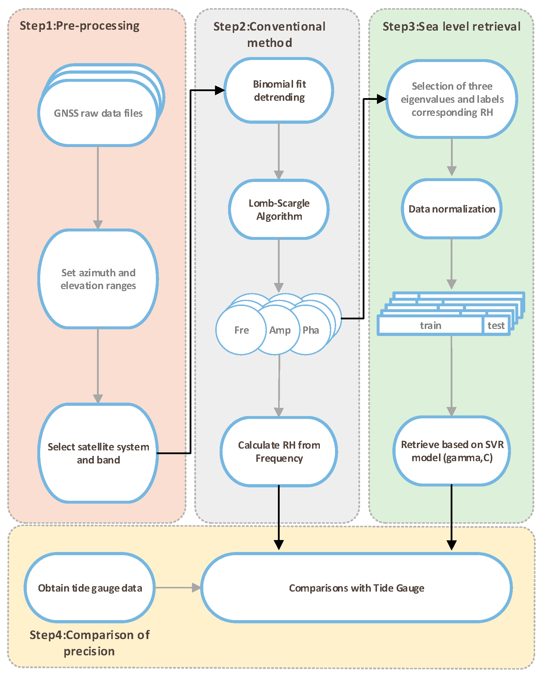
2. GNSS-R Sea Surface Height Retrieval Method
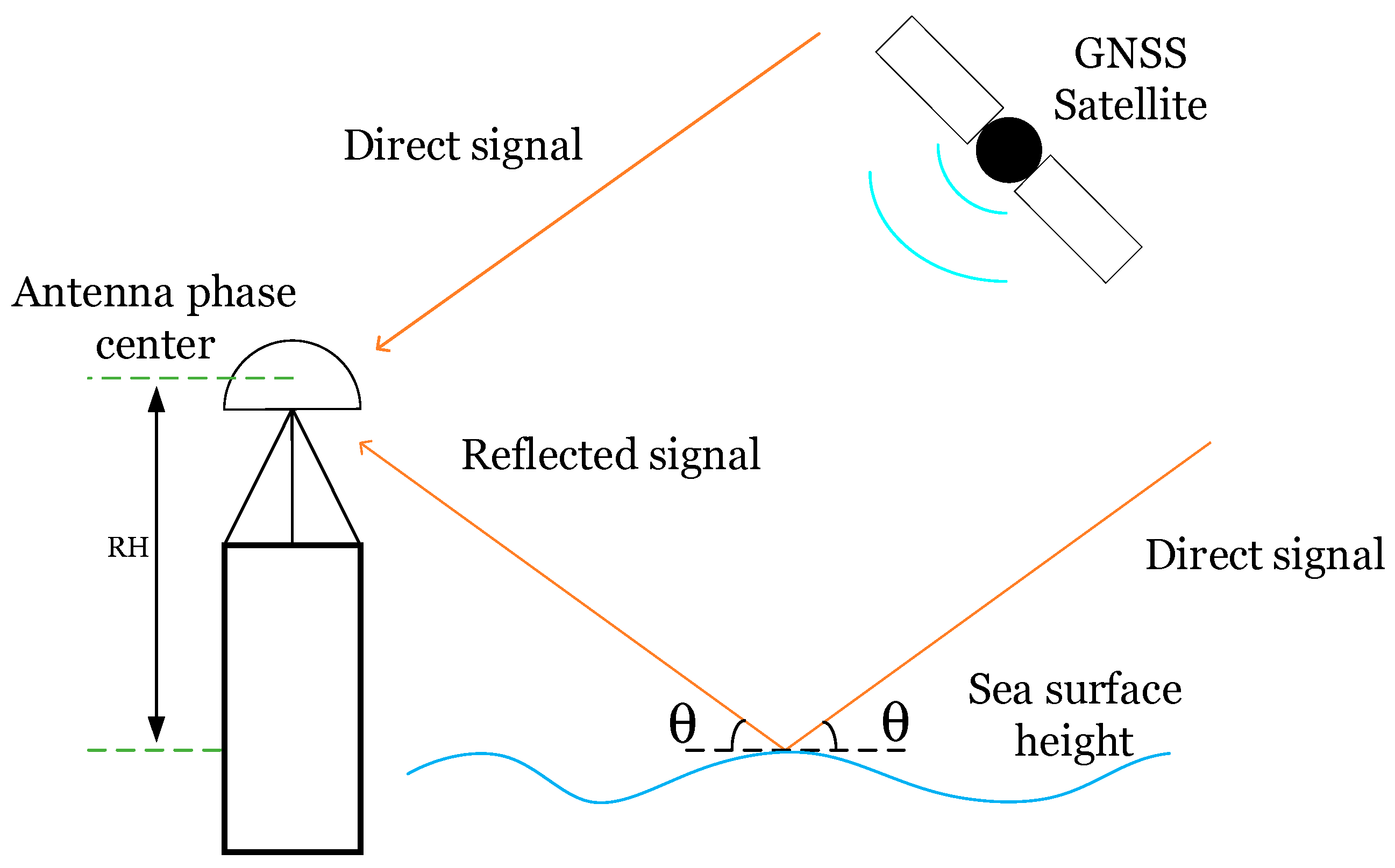
2.1. Principle of GNSS Conventional SNR-Based Altimetry
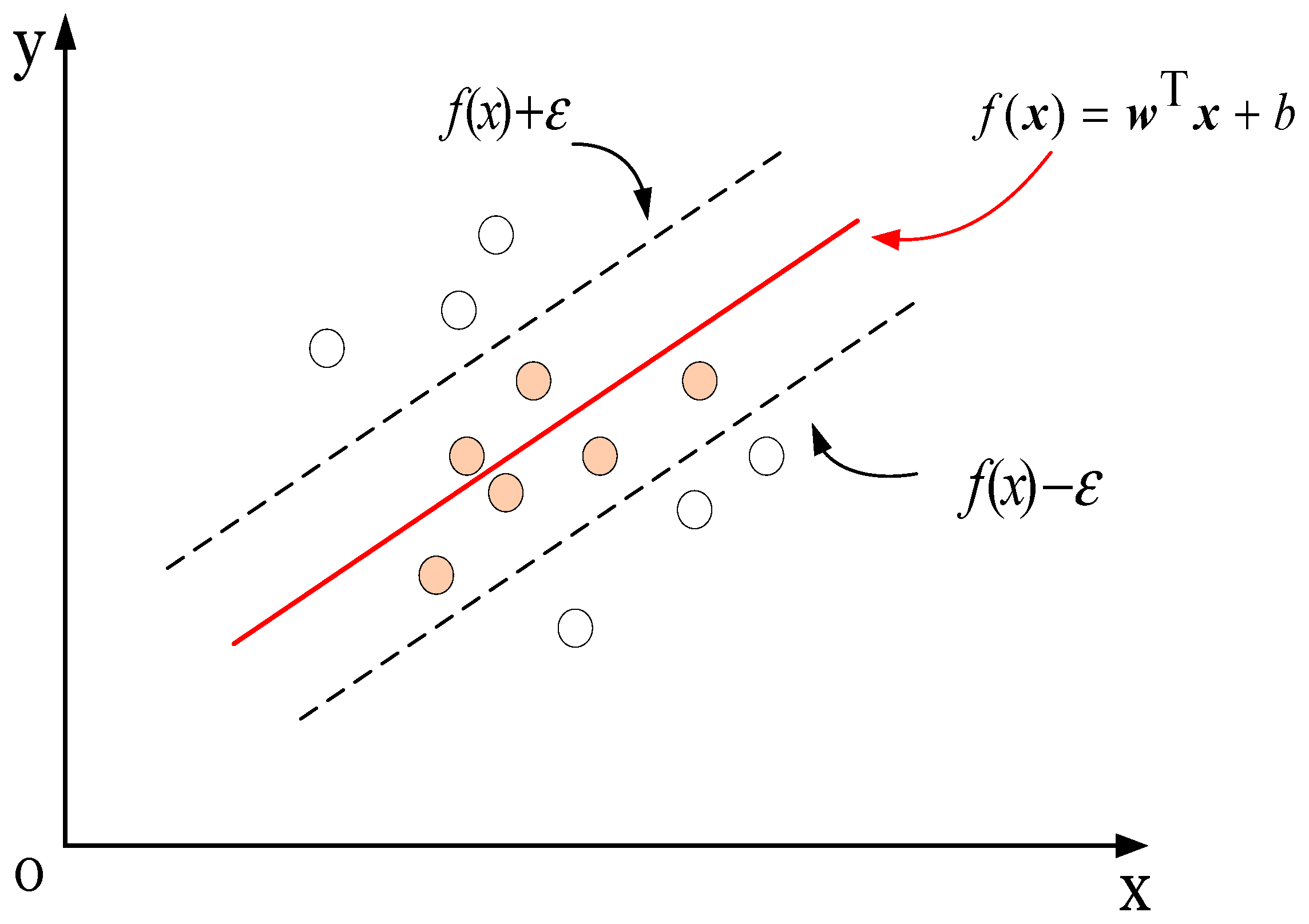
2.2. Support Vector Regression (SVR) Retrieval Principle
3. Experiments and Analysis
3.1. Data Sources and Processing
3.2. Retrieval Process of SVR Model
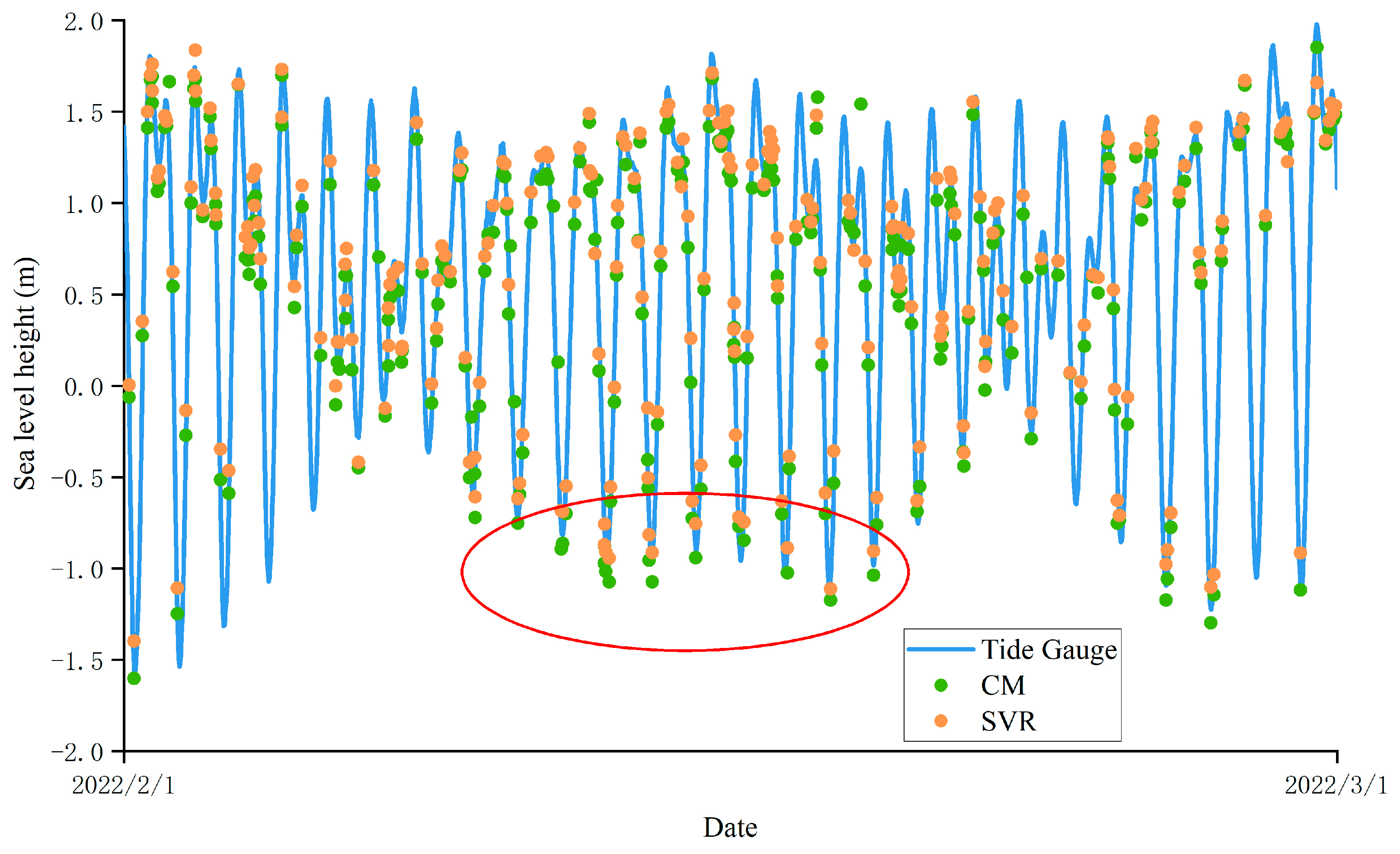
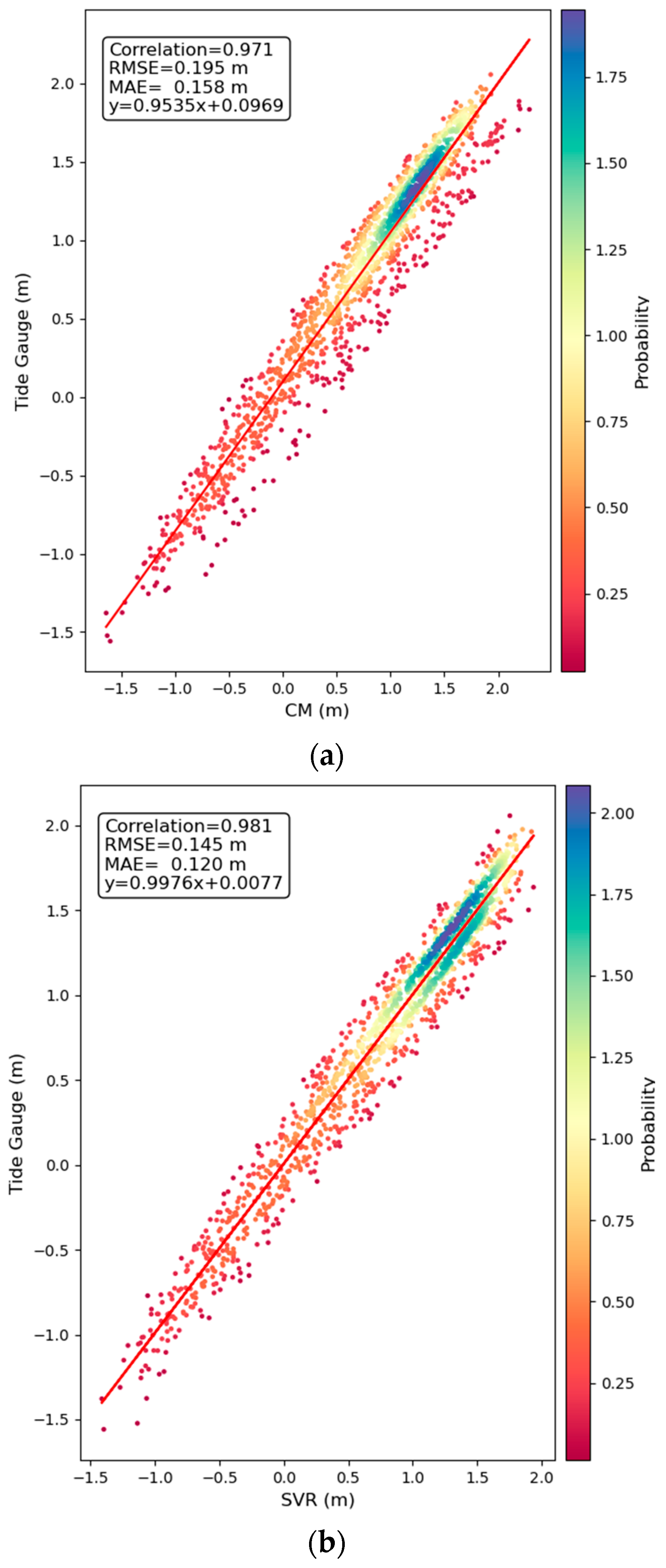
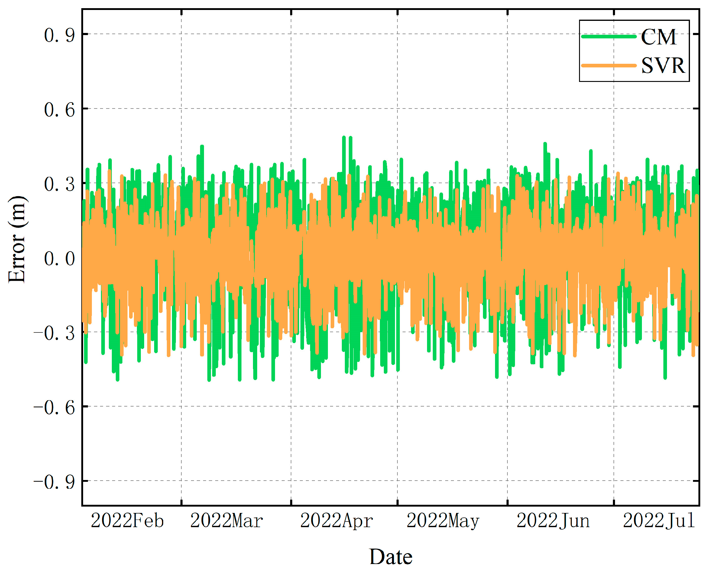
3.3. Results and Analysis
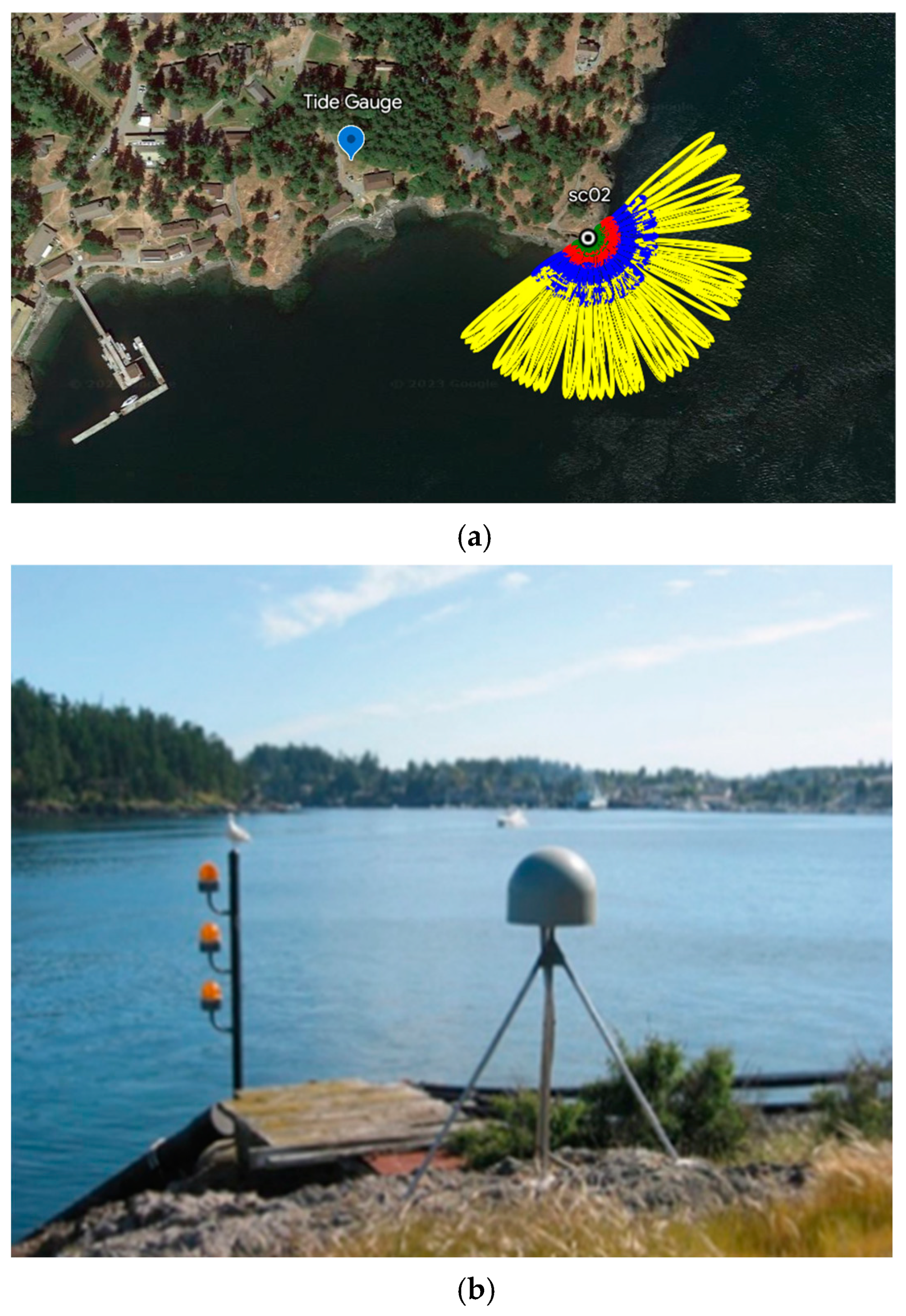
3.3.1. Retrieval Experiment of SC02 Station
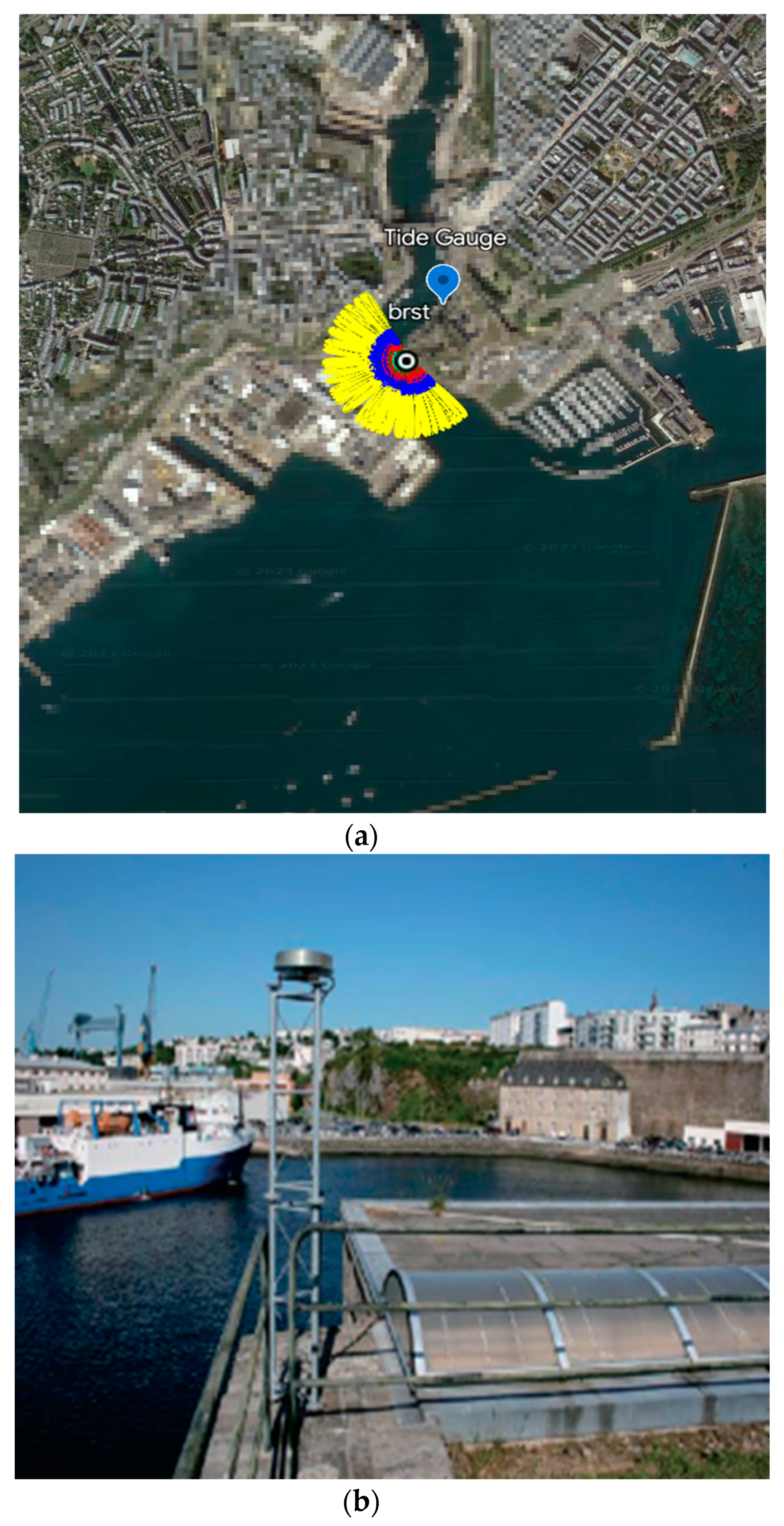
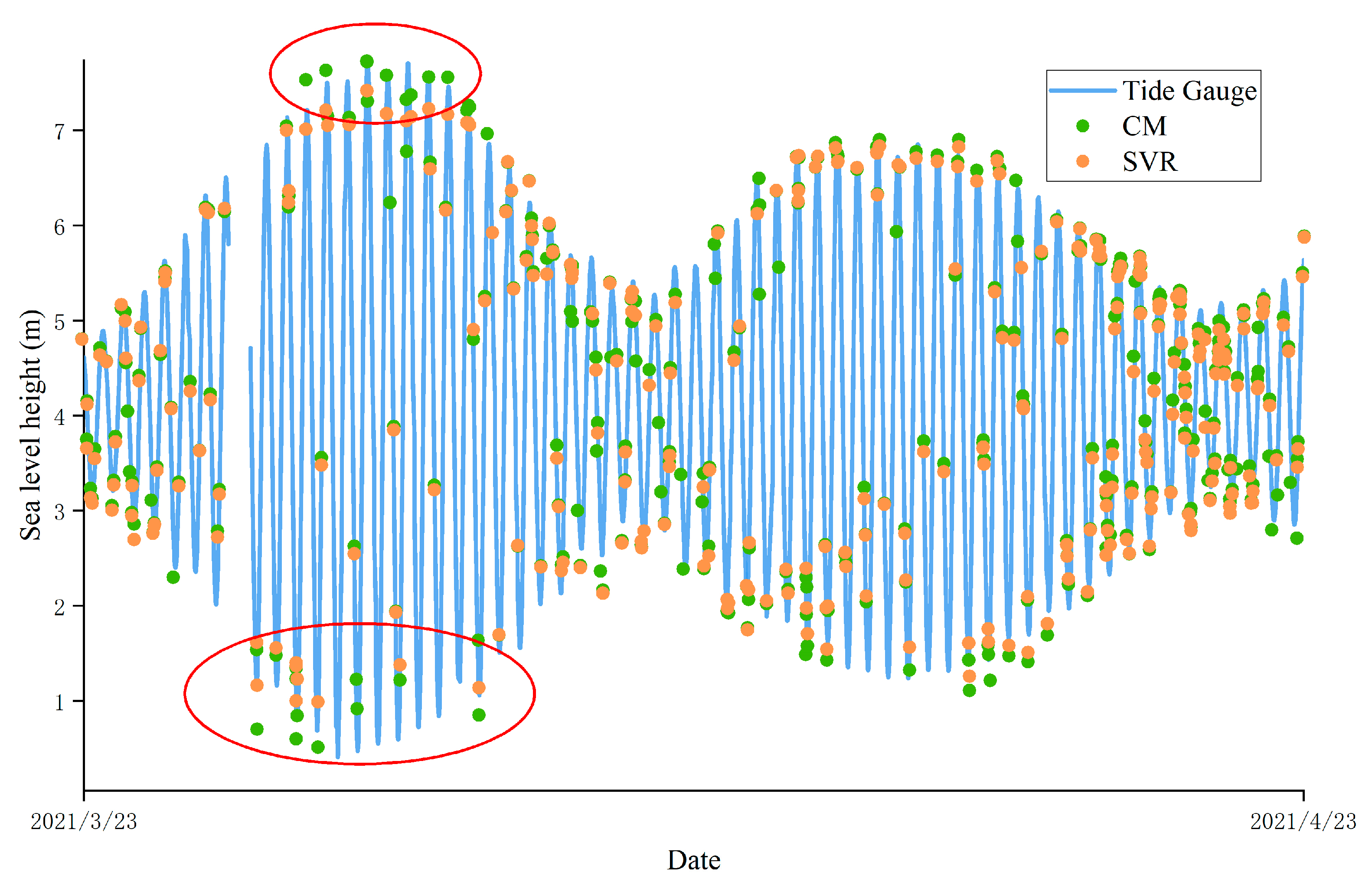
3.3.2. Retrieval Experiment of BRST Station
3.4. Discussion
4. Conclusions
Author Contributions
Funding
Data Availability Statement
Acknowledgments
Conflicts of Interest
References
- Geremia-Nievinski, F.; Hobiger, T.; Haas, R.; Liu, W.; Strandberg, J.; Tabibi, S.; Vey, S.; Wickert, J.; Williams, S. SNR-based GNSS reflectometry for coastal sea-level altimetry: Results from the first IAG inter-comparison campaign. J. Geod. 2020, 94, 70. [Google Scholar] [CrossRef]
- Santamaría-Gómez, A.; Gravelle, M.; Dangendorf, S.; Marcos, M.; Spada, G.; Wöppelmann, G. Uncertainty of the 20th century sea-level rise due to vertical land motion errors. Earth Planet. Sci. Lett. 2017, 473, 24–32. [Google Scholar] [CrossRef]
- Qian, X.; Jin, S. Estimation of snow depth from GLONASS SNR and phase-based multipath reflectometry. IEEE J. Sel. Top. Appl. Earth Obs. Remote Sens. 2016, 9, 4817–4823. [Google Scholar] [CrossRef]
- Yu, K.; Ban, W.; Zhang, X.; Yu, X. Snow depth estimation based on multipath phase combination of GPS triple-frequency signals. IEEE Trans. Geosci. Remote Sens. 2015, 53, 5100–5109. [Google Scholar] [CrossRef]
- Yu, K.; Li, Y.; Chang, X. Snow depth estimation based on combination of pseudorange and carrier phase of GNSS dual-frequency signals. IEEE Trans. Geosci. Remote Sens. 2018, 57, 1817–1828. [Google Scholar] [CrossRef]
- Liu, W.; Beckheinrich, J.; Semmling, M.; Ramatschi, M.; Vey, S.; Wickert, J.; Hobiger, T.; Haas, R. Coastal sea-level measurements based on gnss-r phase altimetry: A case study at the onsala space observatory, sweden. IEEE Trans. Geosci. Remote Sens. 2017, 55, 5625–5636. [Google Scholar] [CrossRef]
- Arroyo, A.A.; Camps, A.; Aguasca, A.; Forte, G.F.; Monerris, A.; Rüdiger, C.; Walker, J.P.; Park, H.; Pascual, D.; Onrubia, R. Dual-polarization GNSS-R interference pattern technique for soil moisture mapping. IEEE J. Sel. Top. Appl. Earth Obs. Remote Sens. 2014, 7, 1533–1544. [Google Scholar] [CrossRef]
- Larson, K.M.; Löfgren, J.S.; Haas, R. Coastal sea level measurements using a single geodetic GPS receiver. Adv. Space Res. 2013, 51, 1301–1310. [Google Scholar] [CrossRef]
- Anderson, K.D. Determination of water level and tides using interferometric observations of GPS signals. J. Atmos. Ocean. Technol. 2000, 17, 1118–1127. [Google Scholar] [CrossRef]
- Zheng, N.; Chen, P.; Li, Z. Accuracy analysis of ground-based GNSS-R sea level monitoring based on multi GNSS and multi SNR. Adv. Space Res. 2021, 68, 1789–1801. [Google Scholar] [CrossRef]
- Larson, K.M.; Ray, R.D.; Nievinski, F.G.; Freymueller, J.T. The accidental tide gauge: A GPS reflection case study from Kachemak Bay, Alaska. IEEE Geosci. Remote Sens. Lett. 2013, 10, 1200–1204. [Google Scholar] [CrossRef]
- Limsupavanich, N.; Guo, B.; Fu, X. Application of RNN on GNSS Reflectometry Sea level monitoring. Int. J. Remote Sens. 2022, 43, 3592–3608. [Google Scholar] [CrossRef]
- Becker, J.M.; Roggenbuck, O. Prediction of Significant Wave Heights with Engineered Features from GNSS Reflectometry. Remote Sens. 2023, 15, 822. [Google Scholar] [CrossRef]
- Altuntas, C.; Iban, M.C.; Şentürk, E.; Durdag, U.M.; Tunalioglu, N. Machine learning-based snow depth retrieval using GNSS signal-to-noise ratio data. GPS Solut. 2022, 26, 117. [Google Scholar] [CrossRef]
- Chew, C.C.; Small, E.E.; Larson, K.M.; Zavorotny, V.U. Effects of near-surface soil moisture on GPS SNR data: Development of a retrieval algorithm for soil moisture. IEEE Trans. Geosci. Remote Sens. 2013, 52, 537–543. [Google Scholar] [CrossRef]
- Zavorotny, V.U.; Larson, K.M.; Braun, J.J.; Small, E.E.; Gutmann, E.D.; Bilich, A.L. A physical model for GPS multipath caused by land reflections: Toward bare soil moisture retrievals. IEEE J. Sel. Top. Appl. Earth Obs. Remote Sens. 2009, 3, 100–110. [Google Scholar] [CrossRef]
- Yan, Q.; Huang, W. Detecting sea ice from TechDemoSat-1 data using support vector machines with feature selection. IEEE J. Sel. Top. Appl. Earth Obs. Remote Sens. 2019, 12, 1409–1416. [Google Scholar] [CrossRef]
- Yan, Q.; Gong, S.; Jin, S.; Huang, W.; Zhang, C. Near real-time soil moisture in China retrieved from CyGNSS reflectivity. IEEE Geosci. Remote Sens. Lett. 2020, 19, 1–5. [Google Scholar] [CrossRef]
- Nievinski, F.G.; Larson, K.M. Forward modeling of GPS multipath for near-surface reflectometry and positioning applications. GPS Solut. 2014, 18, 309–322. [Google Scholar] [CrossRef]
- Lomb, N.R. Least-squares frequency analysis of unequally spaced data. Astrophys. Space Sci. 1976, 39, 447–462. [Google Scholar] [CrossRef]
- Scargle, J.D. Studies in astronomical time series analysis. II-Statistical aspects of spectral analysis of unevenly spaced data. Astrophys. J. 1982, 263, 835–853. [Google Scholar] [CrossRef]
- Strandberg, J.; Hobiger, T.; Haas, R. Improving GNSS-R sea level determination through inverse modeling of SNR data. Radio Sci. 2016, 51, 1286–1296. [Google Scholar] [CrossRef]
- Limsupavanich, N.; Guo, B.; Fu, X. Improvement of Coastal Sea-Level Altimetry Derived From GNSS SNR Measurements Using the SNR Forward Network and T-LSTM Anomaly Detection. IEEE Trans. Geosci. Remote Sens. 2022, 60, 1–13. [Google Scholar] [CrossRef]
- Peng, D.; Feng, L.; Larson, K.M.; Hill, E.M. Measuring Coastal Absolute Sea-Level Changes Using GNSS Interferometric Reflectometry. Remote Sens. 2021, 13, 4319. [Google Scholar] [CrossRef]
- Larson, K.M.; Ray, R.D.; Williams, S.D. A 10-year comparison of water levels measured with a geodetic GPS receiver versus a conventional tide gauge. J. Atmos. Ocean. Technol. 2017, 34, 295–307. [Google Scholar] [CrossRef]
- Larson, K.M.; Gutmann, E.D.; Zavorotny, V.U.; Braun, J.J.; Williams, M.W.; Nievinski, F.G. Can we measure snow depth with GPS receivers? Geophys. Res. Lett. 2009, 36, L17502. [Google Scholar] [CrossRef]
- Drucker, H.; Burges, C.J.; Kaufman, L.; Smola, A.; Vapnik, V. Support vector regression machines. In Advances in Neural Information Processing Systems; MIT Press: Cambridge, MA, USA, 1996; Volume 9. [Google Scholar]
- Vapnik, V.; Golowich, S.; Smola, A. Support vector method for function approximation, regression estimation and signal processing. In Advances in Neural Information Processing Systems; MIT Press: Cambridge, MA, USA, 1996; Volume 9. [Google Scholar]
- Larson, K.M.; Nievinski, F.G. GPS snow sensing: Results from the EarthScope Plate Boundary Observatory. GPS Solut. 2013, 17, 41–52. [Google Scholar] [CrossRef]
- Löfgren, J.S.; Haas, R.; Scherneck, H.-G. Sea level time series and ocean tide analysis from multipath signals at five GPS sites in different parts of the world. J. Geodyn. 2014, 80, 66–80. [Google Scholar] [CrossRef]


| Method | RMSE/cm | MAE/cm | Correlation Coefficient | a | b |
|---|---|---|---|---|---|
| CM | 19.5 | 15.8 | 0.971 | 0.9535 | 0.0969 |
| SVR | 14.5 | 12.0 | 0.981 | 0.9976 | 0.0077 |
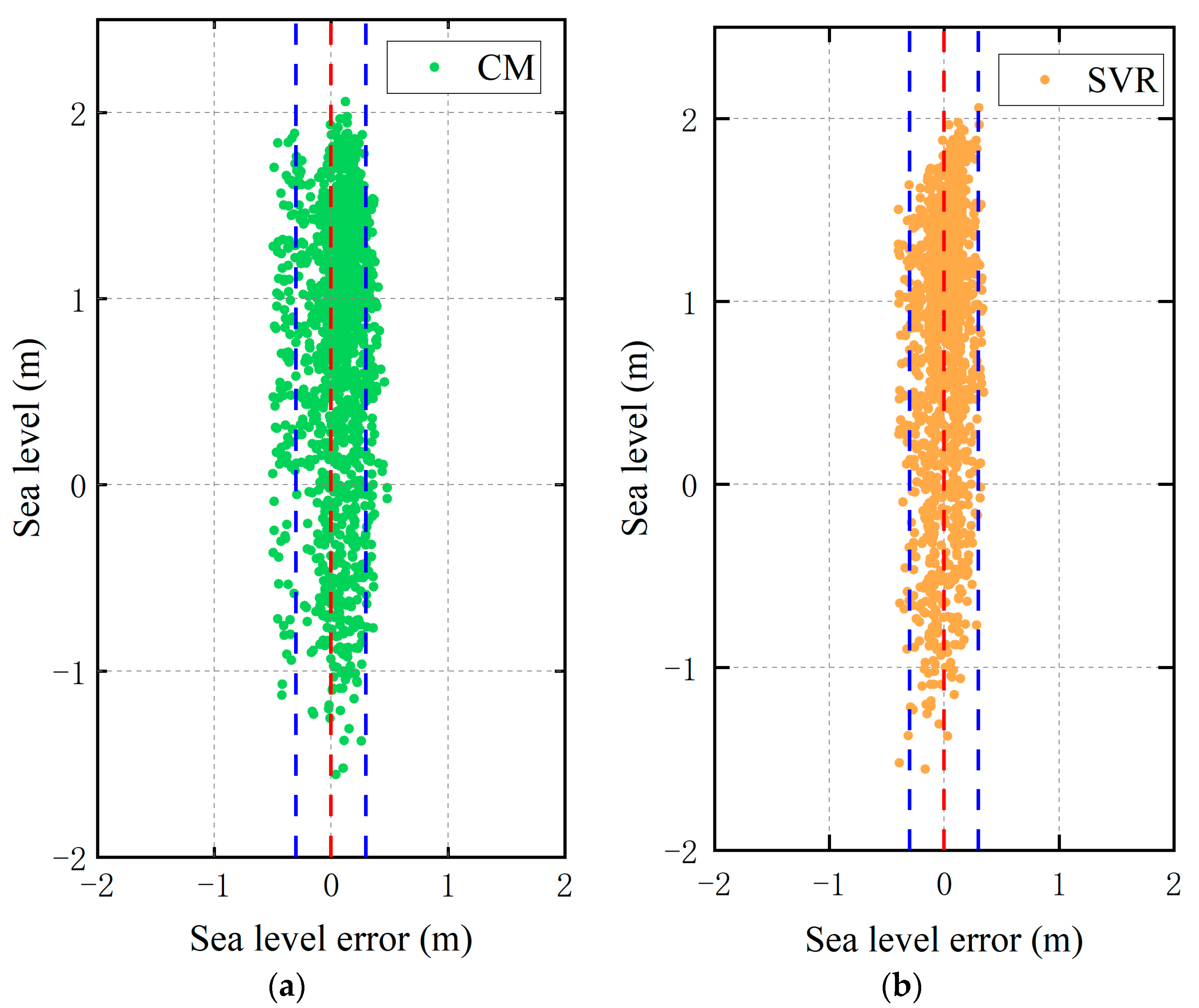
| Method | RMSE/cm | MAE/cm | Correlation Coefficient | a | b |
|---|---|---|---|---|---|
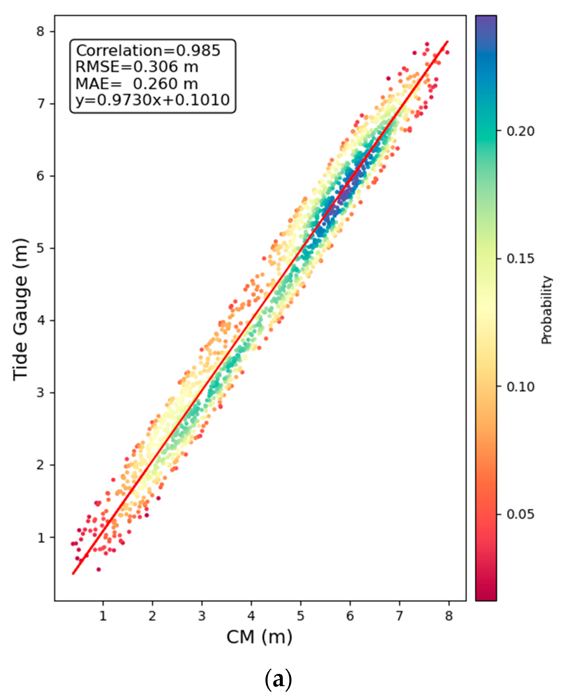
| CM | 30.6 | 26.0 | 0.985 | 0.9730 | 0.1010 |
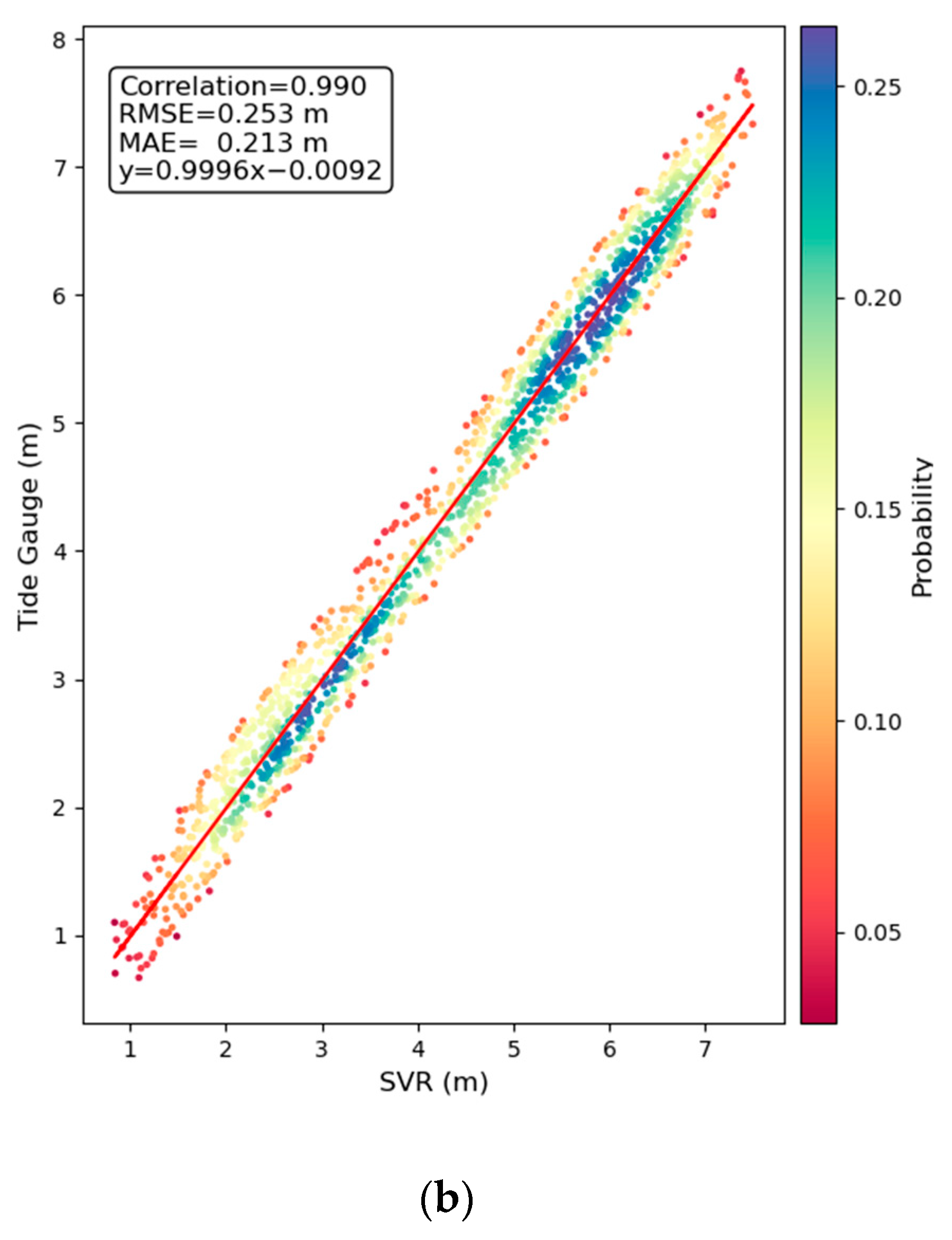
| SVR | 25.3 | 21.3 | 0.990 | 0.9996 | −0.0092 |
Disclaimer/Publisher’s Note: The statements, opinions and data contained in all publications are solely those of the individual author(s) and contributor(s) and not of MDPI and/or the editor(s). MDPI and/or the editor(s) disclaim responsibility for any injury to people or property resulting from any ideas, methods, instructions or products referred to in the content. |
© 2023 by the authors. Licensee MDPI, Basel, Switzerland. This article is an open access article distributed under the terms and conditions of the Creative Commons Attribution (CC BY) license (https://creativecommons.org/licenses/by/4.0/).
Share and Cite
Hu, Y.; Tian, A.; Liu, W.; Wickert, J. Enhancing Sea Surface Height Retrieval with Triple Features Using Support Vector Regression. Remote Sens. 2023, 15, 4029. https://doi.org/10.3390/rs15164029
Hu Y, Tian A, Liu W, Wickert J. Enhancing Sea Surface Height Retrieval with Triple Features Using Support Vector Regression. Remote Sensing. 2023; 15(16):4029. https://doi.org/10.3390/rs15164029
Chicago/Turabian StyleHu, Yuan, Aodong Tian, Wei Liu, and Jens Wickert. 2023. "Enhancing Sea Surface Height Retrieval with Triple Features Using Support Vector Regression" Remote Sensing 15, no. 16: 4029. https://doi.org/10.3390/rs15164029
APA StyleHu, Y., Tian, A., Liu, W., & Wickert, J. (2023). Enhancing Sea Surface Height Retrieval with Triple Features Using Support Vector Regression. Remote Sensing, 15(16), 4029. https://doi.org/10.3390/rs15164029