Abstract
Extensive research on deep neural networks for LiDAR point clouds has contributed inexhaustible momentum to the development of computer 3D vision applications. However, storage and energy consumption have always been a challenge for deploying these deep models on mobile devices. Quantization provides a feasible route, of which current primary research is focused on uniform bit-width quantization without considering different layers or filters’ sensitivity to different bit-widths. This article proposes a novel hybrid compression method based on relaxed mixed-precision quantization, relaxed weights pruning, and knowledge distillation to overcome the limitations of uniform quantization illustrated above, while further improving model accuracy and reducing model memory consumption. It employs a differentiable searching method to search for the optimal bit allocation and weight sparsity, while conducting feature distillation, accordingly considering the feature degradation by pooling operation in point cloud deep models. The proposed method combines three compression techniques to balance the trade-off between compression accuracy and model size. Pruning alleviates the increasing memory consumption problem caused by mixed-precision quantization, while distillation improves compression accuracy without increasing model size. The experiments validate that the proposed method outperforms state-of-the-art typical uniform quantization methods in terms of accuracy with an acceptable and relatively competitive compression performance.
1. Introduction
Three-dimensional point clouds can be conveniently and quickly obtained from LiDAR, and research on deep neural network models based on point clouds has developed rapidly. These models constantly achieve new performance records in tasks, such as object detection and tracking, shape classification, and scene reconstruction and understanding. They have been widely used in several fields, such as autonomous driving, virtual reality, augmented reality, and robotics [1]. However, these deep neural network models require significant amounts of computing and storage resources, making their deployments on resource-limited edge devices (e.g., smartphones or embedded devices) a challenge for practical applications. The main factors affecting the inference speed of neural networks comprise floating point operations per second (FLOPs), memory access cost, and hardware platform-computing resource and memory bandwidth [2]. Research on model compression provides a feasible path to address this issue, but the balancing of the accuracy and model size remains a considerable problem that needs to be solved.
To facilitate the deployment of a deep neural network model, the model compression technique converts a larger complex deep neural network model into a compact compressed model to reduce parameters and inference consumption with minimal accuracy loss. It mainly includes quantization, pruning, knowledge distillation, low-rank factorization, and compact architecture design [3]. In this paper, some related areas are reviewed.
Model quantization [4] converts the high-precision floating-point weights and activation values into low-precision fixed-point values, which include uniform and non-uniform quantization. Uniform quantization indicates that the number of weights or activation quantization bits for each layer is equal. Research on binary neural network has been conducted and has attracted extensive interest from research. Started by BinaryConnect [5], as proposed by Courbariaux et al., numerous binary networks emerged with both binary weights and activation. The BNN (Binarized Neural Networks) [6] presented by Hubara et al. drastically reduces memory size and replaces most arithmetic operations with bit-wise operations. To approximate full precision parameter directly, many works, including XNOR-Net [7], PArameterized Clipping Activation (PACT) [8], and Wide Reduced-Precision Networks (WRPN) [9], have been proposed. To alleviate gradient mismatch, remarkable works, such as Binary Neural Networks+ (BNN+) [10], Bi-Real [11], Half-ware Gaussian Quantization (HWGQ) [12], IR-Net [13], and blended coarse gradient descent (BCGD) [14], have been presented. While mixed-precision quantization refers to assigning different bit widths to each layer/filter, it accounts for the sensitivity to different bit allocations for the different layers or filters. ZeroQ [15] presented a Pareto frontier method to select automatically the bit-precision configuration for mixed-precision settings. Yang et al. [16] built a framework to solve the constrained optimization problem efficiently by using ADMM. Wang et al. [17] introduced a Hardware-Aware Automated Quantization (HAQ) framework that leverages reinforcement learning to automatically determine the quantization policy. Lou et al. [18] proposed a hierarchical DRL-based kernel-wise network quantization technique, AutoQ, to automatically search a quantization bit-width for each weight kernel and choose another quantization bit-width for each activation layer. A new differentiable search architecture was proposed by [19], named Efficient differentiable MIxed-Precision network Search (EdMIPS), with several novel contributions to advance the efficiency by leveraging the unique properties of the mixed-precision network search problem. FracBits [20] is a novel learning-based algorithm to derive mixed-precision models end-to-end under target computation constraints and model sizes, with a fractional status for the bit-width of each layer/kernel and a differentiable regularization term.
Network pruning is another most commonly model compression method, which removes unimportant or redundant parameters or neurons to circumvent over-fitting and reduce the amount of computation and model size. It can be divided into unstructured and structured pruning. Unstructured pruning is a kind of weight parameter pruning ensuring model performance while achieving high sparsity. Structured pruning is a coarse-grained pruning method, such as convolution kernel pruning or channel pruning. The classical framework proposed by Han et al. [21] includes Training, Pruning, and Fine-tuning. Wang et al. [22] aimed to prune networks at initialization to save resources at the training time and proposed Gradient Signal Preservation (GraSP) by preserving the gradient flow through the network. Zhou et al. [23] first studied training from scratch in a fine-grained structured sparse network, maintaining the advantages of both unstructured fine-grained sparsity and structured coarse-grained sparsity simultaneously on specifically designed GPUs. Guo et al. [24] proposed a novel differentiable method for channel pruning, named Differentiable Markov Channel Pruning (DMCP), to efficiently search the optimal sub-structure that is directly optimized by gradient descent with respect to standard task loss and budget regularization. Lin et al. [25] proposed a novel filter pruning method by exploring the High Rank of feature maps (HRank), which is mathematically formulated to prune filters with low-rank feature maps on the principle that low-rank feature maps contain less information.
Knowledge distillation, a method of transferring knowledge from a teacher model to a student model, typically includes knowledge, distillation algorithm, and teacher–student architecture. The concept was formally proposed by Hinton et al. [26] in 2015. There have been many studies on knowledge distillation, including knowledge distillation based on response, features, and relationships, and other complex algorithms, such as adversarial distillation, multi-teacher distillation, cross-model distillation, graph-based distillation, data-free distillation, and NAS-based distillation. These algorithms have been widely applied to different scenarios. Passban et al. [27] proposed a combinatorial attention technique that fuses the teacher-side information and takes each layer’s significance into consideration, performing distillation between the combined teacher layers and those of the student. Tan et al. [28] introduced two novel mechanisms: an Alternate Attention-Transfer Mechanism (AATM) and a Semantic Distillation Mechanism (SDM) to help a generator bridge the cross-domain gap between text and image. Yuan et al. [29] systematically developed a reinforced method to dynamically assign weights to teacher models for different training instances and optimize the performance of student models.
Neural Architecture Search (NAS) can automatically design high-performance network structures that search for the optimal network structure given a set of candidate neural network structures, called a search space. It effectively solves the parameter tuning problem of neural network and includes three important modules, named search space, search strategy, and performance estimation. Early NAS methods are primarily based on reinforcement learning or evolutionary algorithms. Then, a weight-sharing strategy is gradually developed in the field of neural structure search. The researchers back-propagate the structural coefficients in a continuous differentiable search mode. Liu et al. [30] proposed a differentiable architecture search (DARTS) to solve the neural structure search problem from a completely new perspective. Ye et al. [31] proposed a simple but efficient regularization method, termed as Beta-Decay, to regularize the DARTS-based NAS searching process. Zhang et al. [32] formulated a stochastic hyper-gradient approximation for differentiable NAS and theoretically showed that the architecture optimization with the proposed iDARTS is expected to converge to a stationary point. Li et al. [33] redesigned the DARTS framework to automatically refill the skip connections in the evaluation stage, resolving the performance degradation caused by the absence of skip connections by introducing an adaptive channel allocation strategy. Qin et al. [34] proposed a Graph-differentiable Architecture Search model with Structure Optimization (GASSO), which allows the differentiable search of the architecture with gradient descent and can discover graph neural architectures, employing graph structure learning as a denoising process in the search procedure.
Although quantization can reduce the memory consumption and improve the inference speed, the extremely low bit quantization can especially lead to a significant accuracy reduction. Current uniform quantization methods neglect the fact that different layers normally need different quantization bits to better represent the feature map. To overcome the limitations of uniform quantization, this paper employs the mixed bit-width quantization method on a point cloud deep model. Given the advantages and disadvantages of mixed bit-width quantization, this article comprehensively compresses point cloud deep network models using quantization, pruning, and knowledge distillation, which considers the sensitivity of quantization for different layers by adopting mixed bit-width quantization, further reduces the size of the mixed bit-width quantization model using pruning, and leverages knowledge distillation to optimize the model performance, accounting for the special characteristics of point cloud. So, a hybrid compression method is proposed, which could outperform the single compression mode with uniform quantization and balance accuracy and consumption.
The main contributions are as follows.
- (1)
- To circumvent the problem of complex search for discrete sparsity and bit space, a novel differential search for optimal weight sparsity and optimal bit allocation of weight and activation is specially designed, with a cascade of ‘pruning before quantization’.
- (2)
- To alleviate the performance degradation of the point cloud deep compression model caused by pooling operation based on theoretical analysis, the feature knowledge distillation method is utilized to recover the pooled feature fidelity.
- (3)
- Experiments are conducted on the three typical datasets of ModelNet40, ShapeNet, and S3DIS for classification, part-segmentation, and semantic segmentation, respectively, to validate the efficiency and scalability; model complexity is also analyzed.
2. Methods
The flowchart of the proposed hybrid compression framework is shown in Figure 1. Figure 1a provides a general workflow. When inputting the point clouds in the deep model, the full precision model is pruned and then quantized with mixed bit-width differentially. During backward propagation, pooled feature-based distillation loss is added. It mainly includes three subsections: weight pruning, mixed-precision quantization, and knowledge distillation. The core idea of this design is to overcome the limitation of uniform quantization using the same bit-width for different layers; thus, this paper adopted the mode of mixed bit-width quantization and further introduced pruning to optimize additional memory brought overhead by the mixed bit-width. Feature-based knowledge distillation was used to alleviate the performance degradation caused by the point cloud pooling aggregation. Figure 1b is the proposed hybrid compression model on a typical PointNet backbone. Weight pruning was performed before mixed bit-width quantization, while activation directly underwent mixed bit-width quantization. Knowledge distillation was mainly implemented by the feature distillation method and was further optimized in two stages using the response-based distillation method.

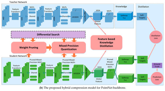
Figure 1.
The flowchart of the proposed hybrid compression method for the point cloud deep model.
2.1. Relaxed Cascading Compression
Compression mainly targets the convolutional layers and fully connected layers of the convolutional networks. The convolutional layers and fully connected layers contain most of the model parameters. By compressing and quantizing these layers, we can significantly reduce the storage and computation cost of deep neural networks, making them more practical for various applications.
Both convolution in deep convolutional networks and fully connected operations can be represented as
where denotes the input, is the output, and is the convolution or linear mapping. To implement the cascading compression proposed by this paper,
where is the mixed-precision quantization function, is weight pruning function, is the mixed-precision input, and denotes the mix-quantization weights after pruning.
The optimal bit/sparsity search process for convolution/fully-connected layer is shown in Figure 2. The compression for weights uses a kind of cascading type of ‘pruning–quantization’, while the activation implements mixed quantization. The overall network is fully differentiable and could find optimal bit/sparsity allocation from a given discrete and large search space without proxies. To further speed up the search process, layer-wise pruning or quantization was implemented.
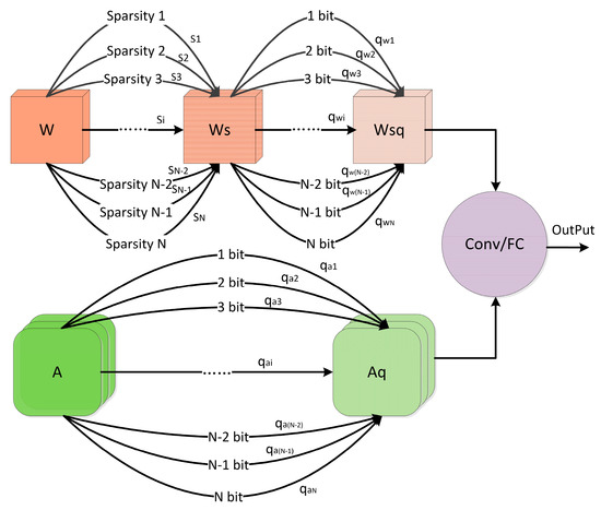
Figure 2.
The optimal differential search module.
2.1.1. Relaxed Mixed-Weight Pruning
Weight pruning is the process of removing relatively unimportant values from the weight matrix and then conducting fine-tuning. The common practice is to directly assign a value of 0 to weight values that are close to 0. The threshold can be determined by various criteria, such as using the percentage of the maximum absolute value of the weights. In theory, the redundancy of weights may vary across layers, so the above pruning percentage should also be adjusted accordingly. To search for the optimal sparsity of weights at each layer of the network,
where is the cardinality of the sparsity candidate space. To derive the layer-wise sparsity configuration of the compressed model, the complex combinatorial optimization problem needs to be considered. The cascaded compression process of ‘pruning–quantization’ for weights with the binary characteristic of search space inevitably leads to a complex combinatorial optimization. The binary search process is suggested to be relaxed into a continuous one [19,30],
Then, the configuration parameter could be reformulated as
where is a set of real configuration parameters. This means that optimal configurations can be searched within a new continuous space formed by combining the following quantization relaxation spaces, and they can be learned together through the gradient descent method. After optimization, we selected the branch/sparsity with the highest value of .
2.1.2. Relaxed Mixed Quantization
After pruning, the sparse weights were then implemented with mixed-precision quantization. As illustrated above, the bit configuration spaces of weights and activation were also relaxed into continuous ones to circumvent combinatorial optimization problems.
where , , , and . Similarly,
and
can be expressed by
From Equations (4) and (6), it can be concluded that could be substituted by the real parameters of .
2.2. Knowledge Distillation
Knowledge distillation is used to solve the problem of significant performance degradation caused by the symmetric operation of pooling in point cloud deep networks. On this paper, we elaborated from three aspects of theoretical analysis, feature-based distillation, and response-based distillation.
2.2.1. Theoretical Analysis
When quantizing from full-precision 32-bit floating point to low bit, such as 1 bit, 2 bits, and 4 bits, feature information loss is inevitable. Information entropy can reflect the feature representation ability, which can be expressed as
where the range of values is
and the maximum value relates to the number of categories k. It can be concluded that, as the quantization bit decreases, the maximum value of entropy also decreases, which means that the ability to represent features to the largest extent is limited. Therefore, quantization inevitably leads to a decrease in the ability of feature representation. As the number of quantization bit decreases, the extent to which the feature representation ability decreases will also vary. The fewer the digits, the more pronounced the decrease. To provide a clearer illustration, consider binary quantization as an example, and others that are similar; see further details in Appendix A.
2.2.2. Feature-Based Distillation
As an important type of knowledge in representation learning, the feature knowledge of a hidden layer can better guide the training of a student network. Feature distillation considers the selection of intermediate hidden layers. For quantized networks, since the network structure is the same as that of a corresponding full-precision network, the corresponding layers’ feature can be used to constitute the distillation loss directly.
This paper selected cross-entropy loss considering the above theoretical analysis. Meanwhile, a 1-norm distance was also selected for comparison. To derive the cross-entropy loss of the pooled feature,
where
and
denote the pooled feature of the teacher and student models, respectively. The probability estimation uses kernel density estimation (KDE) based on cosine kernel,
2.2.3. Response-Based Distillation
The feature map of the hidden layer is denoted as , and the output after the Softmax layer is , where
is the learned weights’ matrix. The predicted probability of the network output is
where is the temperature hyper-parameter, which controls the dependence on the soft target, and the distribution of the soft target becomes more uniform as the value increases. is the learned optimization parameter. The distillation soft target loss is
where the subscripts
and
denote full precision and quantization, respectively.
denotes the label. The distillation loss is
where is the cross-entropy prediction loss term. is a hyper-parameter that balances the importance of both.
2.3. Training
2.3.1. Loss Function
In addition to the distillation loss analyzed above, the impact of quantization and weight pruning on the size of the model should also be considered. Therefore, introducing a constraint on model complexity can better balance the accuracy and complexity. Model complexity uses an improved form based on [19],
where
and
are the bit widths of activation and weights, respectively.
denotes the weight sparsity.
When using a pre-trained full-precision model as the teacher model, it is important to add the loss functions designed in
Section 2.2.2
and
Section 2.2.3
together as the total loss function for the training of the hybrid compression network.
where and are the hyper-parameters measuring the importance of the pooled feature loss and model complexity, respectively. When using response-based distillation loss, should be replaced by .
2.3.2. Training Strategy
This article adopted a two-step strategy for the training of the hybrid compression model, with cascaded knowledge distillations. In the first step, a feature-based knowledge distillation method was used to train a quasi-optimal model to achieve the quasi-best performance. In the second step, a response-based knowledge distillation method was used to fine-tune the previously trained model. During knowledge distillation, the teacher model (i.e., full-precision network) was pre-trained and the knowledge was transferred from the pre-trained full-precision model to the hybrid compression model. See the detailed algorithm Algorithm A1 in Appendix B.
2.3.3. Parameter Setting and Datasets
The methods presented were all trained and validated using the same configuration. The hardware configuration was Intel® CoreTMi5-9400, memory of 16 GB; Graphics: NVIDIA GeForce RTX 2080Ti. We took the typical PointNet [35] as an example and then extended it to other backbones. The training and validation of point cloud deep models were implemented in PyTorch 1.5.0. All of the networks were trained from scratch. During training, the batch size was set as 64 and the epoch number of the total two phases was set as 200 epochs for classification, 250 epochs for part segmentation, and 128 epochs for semantic segmentation. To update the network parameters, the optimizer used Adam with an initial learning rate of 0.001 by cosine annealing decay. For the relaxing parameters , all initial values were set as 0.01 and their learning rate was initialized as 0.0001.
The datasets of ModelNet40 [36], ShapeNet [37], and S3DIS [38] were used in the experiments, which were used for shape classification, part-segmentation, and semantic segmentation, respectively. Specifically, there exist 12,311 artificial objects of 40 categories with 3D CAD shapes for ModelNet40, which contains 9843 samples for training and 2468 samples for testing. ShapeNet contains 16 categories of 3D shapes amounting to 16,881, most of which consist of 2 to 5 parts with a total of 50 parts. The S3DIS dataset was acquired by 3D scans of Matterport scanners, including 271 rooms of 6 regions, and each scanning point is annotated with one of 13 classes of semantic labels, such as table, chair, wall and floor.
2.3.4. Assessment Indicator
Accuracy was calculated by
where is the number of samples/pixels where the prediction is positive and the actual is positive, denotes the number of samples/pixels where the prediction is positive and the actual is negative, and and have similar representations.
The Intersection over Union (IoU) is the ratio of the intersection and union of the segmentation result and the ground truth for category :
where is the number of true positive cases, is the number of false positive cases, and is the number of false negative cases.
The mIoU is the mean of IoU,
where is the number of categories of the segmentation results.
3. Experimental Results
This section provides the results of the ablation experiment, comparative experiment, extended experiment, visualization, and complexity analysis.
3.1. Ablation Experiment
The proposed hybrid compression method comprise pruning, quantization, and knowledge distillation, and this section implements ablations of these three parts.
3.1.1. Pruning Ablation
To validate the effectiveness of pruning, we adjusted the sparsity space on the basis of fixed quantization space to prune the weights. Relaxed mixed quantization is implemented with the weights’ bits space and activation bits space . The bits for activation are more sensitive than those for the weights, so the bits space for activation started at two bits and one bit for the weights. Considering the overall compression performance, the highest bit was set as 4. Larger bits may result in more memory consumption. The following experiments used the above weights’ bits space and activation bits space without any special illustration. Table 1 presents the ablation results of the relaxed mixed pruning. To indicate the priority of the relaxed mixed pruning, uniform pruning was provided with a layer-wise threshold factor ranging from 0.025 to 0.500. To compare with uniform pruning, the average layer-wise threshold factor was used by averaging all the layers’ sparsity of the trained model. The approximating average threshold factor was derived by adjusting the range of the sparsity space. From the table, it can be concluded that, when the threshold factors are approximately equal, the mixed pruning results are better than the uniform pruning method. Figure 3 shows the weights’ sparsity variations of different layers during training with an approximated average threshold factor of 0.400, indicating that the weights’ sparsity of different layers has different sparse sensitivity.

Table 1.
Ablation results of relaxed mixed pruning.
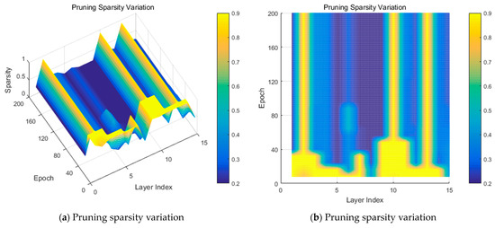
Figure 3.
Layer-wise pruning sparsity variation during the training process.
3.1.2. Quantization Ablation
To validate the efficiency of relaxed mixed quantization, compression with only quantization was implemented with different complexity factors. Table 2 illustrates the quantization ablation results with a complexity factor ranging from 1 × 10⁻¹ to 1 × 10⁻⁹. It can be concluded that, as the complexity factor’s value decreases, the number of bits roughly increases. This indicates that, with a larger regularization of the complexity, the bit width becomes smaller, and the bit width becomes larger if the regularization of complexity is smaller. Figure 4 presents the bit variation during training for both weights and activation. It indicates that the activation needs larger bits than weights (i.e., with a larger yellow area) and activation is much more sensitive than the weights.

Table 2.
Ablation results of relaxed mixed quantization.
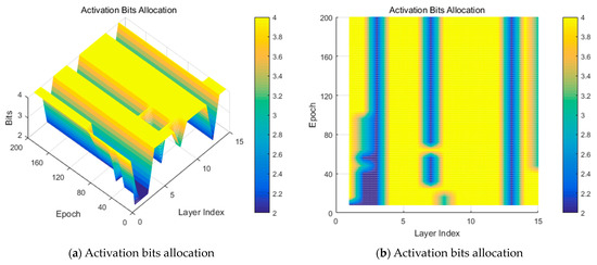
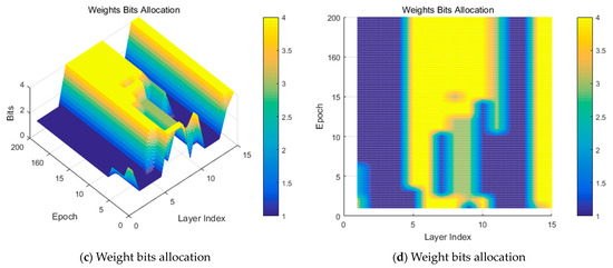
Figure 4.
Bit variation for mixed-precision quantization during training.
3.1.3. Distillation Ablation
This section presents the knowledge distillation ablation results based on feature and response. Table 3 presents the distillation results with complexity factor of 1 × 10⁻⁶. Feature-based distillation includes 1-norm distance (type I) and cross-entropy loss (type II). Either with only feature distillation or both, the accuracy is consistently improved, achieving the highest value of 87.8. Table 4 provides the results of type II feature distillation. The accuracy improved, achieving the highest value of 87.3 for the complexity factor 1 × 10⁻⁶. The above analysis reveals the efficiency of the distillation.

Table 3.
Distillation ablation results for type I.

Table 4.
Distillation ablation results for type II.
3.2. Comparative Experiment
It can be concluded from Table 5 that the highest accuracy value for the proposed hybrid compression method was 88.1, which is closer to that of full precision. It reduces the model size with an average bit of 3.000 for weights and 3.933 for activation and sparse weights. Figure 5 shows the training error curve during the training process. Compared to the uniform quantization method with the highest accuracy, the proposed hybrid compression converges faster and even better than the full precision one, with a value of epochs of less than about 100.

Table 5.
Comparison between the typical uniform quantization and hybrid compression methods.
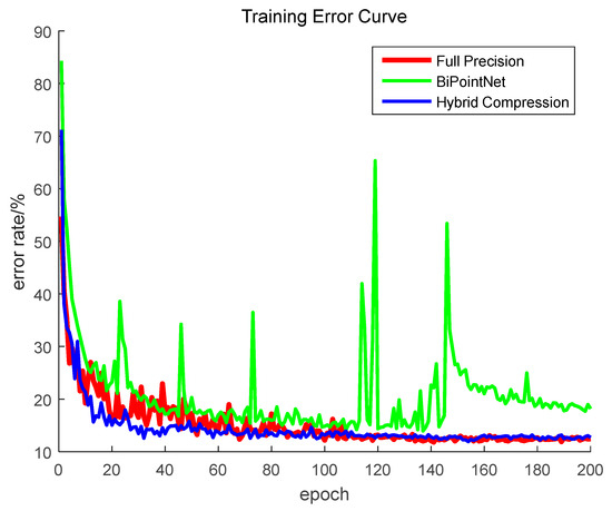
Figure 5.
Training error variation curves during training.
3.3. Extended Experiment
This section extends the experiments of the classification task on PointNet backbone to segmentation tasks and other backbones.
3.3.1. Segmentation Experiment
Table 6 provides the results of part-segmentation. The proposed hybrid compression outperformed all of the uniform quantization methods with an average accuracy of 79.9, while the average accuracy is 53.3 for BNN(1|1 bit), 73.3 for HGWQ (3|3), and 75.0 for HGWQ (4|4). The hybrid compression method has average weights bits of 2.26, average activation bits of 3.06, and average weights sparsity of 24.8%, and the model size is also competitive.

Table 6.
Part-segmentation results.
Table 7 indicates that the semantic segmentation for hybrid compression method is also more competitive than uniform quantization. It has the highest mean mIoU of 41.9, overall accuracy of 73.8, average weights bits of 2.1, average activation bits of 2.8, and average weights sparsity of 5.6%. It is competitive not only in terms of accuracy but also model size/memory. The segmentation for six areas also has a better performance, although the column IoU is somewhat smaller than the one of HGWQ 4|4.

Table 7.
Semantic segmentation results.
3.3.2. Other Backbones
The validation of shape classification on other typical popular backbones was also implemented. Table 8 shows the detailed results. The complexity factor was set as 0.5 × 10⁻⁶. This indicates that mixed precision and sparsity can improve the accuracy to meet different layers’ sensitivity to the bit number and weight sparsity.

Table 8.
Classification comparison of the different backbones.
3.4. Visualization
To directly show the effects of the proposed hybrid compression, this section shows parts of the segmentation results.
3.4.1. Part-Segmentation
Figure 6 shows the part-segmentation results for three samples. The segmentation errors are concentrated on the handle of handbag. For BNN, it is almost entirely wrongly segmented, while for HGWQ and the proposed methodology, the situations are much better. However, compared to HGWQ, the proposed method has much less noise on the handle. The situation is similar to the cases of the motorbike and skateboard. For example, the segmentation of the fuel tank and headlamp for the motorbike and the board edge for the skateboard are much better in the proposed method.
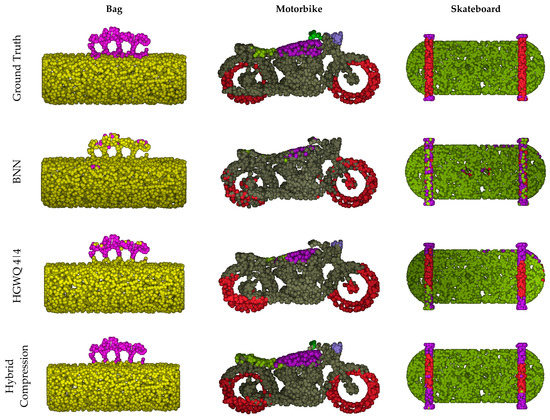
Figure 6.
Part-segmentation results.
3.4.2. Semantic Segmentation
Figure 7 and Figure 8 show the segmentation of different areas. For auditorium 1 of Area 2, the segmentation of roof, row of chairs, projector, and roof beams is better in the case of hybrid compression than that of others. For example, compared to the ground truth, part of the roof in BNN is wrongly classified as a wall and in HGWQ as ground, while in the proposed method, the roof segmentation is more pure. The wall segmentation in BNN is the worst, while in HGWQ and the proposed method, it is much better. The proposed method has a more accurate result for the boundaries between roof and wall, while HGWQ has obvious over-segmentation and under-segmentation. For office 5 of Area 5, the proposed method also outperforms others. For example, the segmentation of areas around the door, labeled with a brown color, is more accurate in our hybrid compression method, while in HGWQ, part of the area is misclassified as blue color and, in BNN, it is almost completely wrong. The segmentation of the desk and bookshelf inside are also more accurate in the proposed method, while in BNN, the desk is completely segmented as ground floor. HGWQ is a little better, but most parts are not properly segmented by correctly labeling similar objects inside the office. The proposed method also has limitations, e.g., the three parts marked with the brick blue color on the roof in the ground truth are also not segmented.
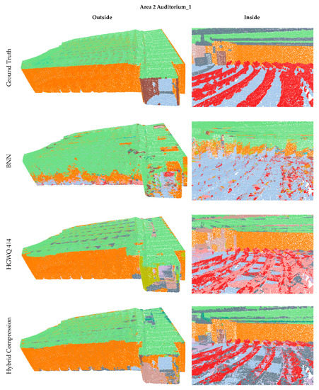
Figure 7.
Semantic segmentation results I.
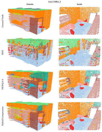
Figure 8.
Semantic segmentation results II.
3.5. Complexity Analysis
Complexity regularization during training could balance the accuracy and memory size. Figure 9 presents the complexity evolution with increasing epochs. It can be concluded that, regardless of any complexity factor value, the complexity approximately approaches a relatively stable status with a larger epoch number. When the complexity factor is smaller than 1 × 10⁻⁵, the smaller the value, the faster the complexity reaches a steady state. As the complexity factor value decreases, the complexity value of the steady state gradually increases, which indicates the regularization of the complexity term decreases. When the complexity factor is greater than 1 × 10⁻⁴, the larger regularization causes the model complexity to change a little and maintain a lower state with the increase in epochs.
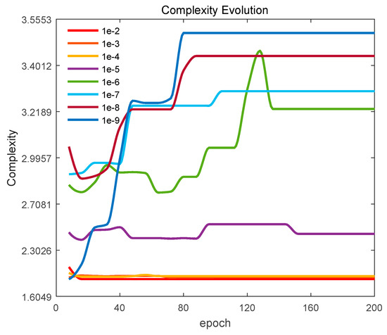
Figure 9.
Complexity evolution.
Table 9 shows the complexity for uniform quantization and the proposed hybrid compression for PointNet inference classification network. Compared to the extreme quantization binary model of BNN, which has the highest speedup time of 53.0 and compression time of 23.2, the hybrid compression method is more memory-demanding and has a lower speedup. With the highest classification accuracy of 88.1%, the PointNet inference model size is about 0.44 Mb and the compression ratio is 7.9. Only binary quantization can use an efficient bit-wise operation; other quantization methods larger than 1 bit also have greater flops. However, the accuracy of the binary method is far from satisfactory. Although the optimization-based binary method could achieve a higher accuracy, e.g., XNOR-Net and BiPointNet, both of them consume more memory and need complex training optimization. The training of the proposed hybrid compression method is differential and much easier, although the average bit allocation is relatively larger. Weight pruning could also add sparsity to weights and efficiently skip the computation on zeros. While TTQ and TWN are both weights-only ternary methods, the complexity improvement is limited and the speedup ratio relates to the sparsity s. The situation is also similar in the proposed hybrid compression method. The expression with variable s is just an approximation. It does not take into account the float numerical addition; so, it should be slightly larger than 443.38 × (1-s). The parameter for the proposed model is less than 0.15 × Nw, where Nw denotes the weights’ mixed bits, because the weight sparsity could also lead to a lower model size consumption. Thus, the compression ratio is larger than 23.2/Nw.

Table 9.
Complexity analysis for the uniform and proposed hybrid inference networks.
4. Discussion
The proposed hybrid compression method aims to solve the problem of uniform quantization that the differents layers are forced to have the same sensitivity to bit allocation. From classification to segmentation on PointNet, and from PointNet to other typical backbones, the hybrid compression based on differential relaxed mixed quantization and mixed pruning can efficiently improve accuracy. Meanwhile, the pooling feature distillation also presents benefits. Increasing bits inevitably results in more memory consumption; so, we combined weight pruning to decrease the model size further. From our experiments, the mixed weight sparsity factor for classification and semantic segmentation was always less than 10% and contributed less to the model size. For part-segmentation, the weight sparsity of most types was greater than 20%, even with the highest value of 42.8% for cap; this pruning is efficient to compensate for the model size increase with mixed bits. To achieve a higher accuracy without extra memory consumption, distillation plays an important role. With a classification accuracy ranging from 86% to 88% on PointNet, the effort to improve is quite difficult. However, distillation can achieve this to obtain an remarkable 88.1%, which is nearly equal to the accuracy of full precision, at 88.2%, with only 0.1% of difference.
Compared to previous research, the proposed hybrid compression method takes into account the commonality of network quantification and the particularity of the point cloud model. Compared to mixed precision quantization, uniform quantization methods, including BNN, XNOR-Net, IR-Net, Bi-Real, BiPointNet, TTQ, TWN, and HGWQ, are simpler since the different layers share the same bit width and the bit width is assigned before, e.g., BNN, XNOR-Net, IR-Net, Bi-Real, and BiPointNet assign 1 bit and TTQ and TWN assign 2 bits. These uniform quantization methods consider different layers that can have the same bits. The proposed hybrid compression method uses mixed bit-width quantization, and the bit allocations for different layers can be changed according to the actual situation, named “Assign on demand”. Uniform quantization, especially extremely low-bit quantization, has a significant accuracy drop, although it has a higher compression ratio. An extremely low bit will inevitably cause a vast loss of representation. In the improvement of performance, optimization-based methods have dominated; however, the optimization process is always complex and time-consuming, e.g., BiPointNet, the state of the art in point cloud model compression, cannot obtain a closed solution of the optimized parameters, and hundreds of thousands of Monte Carlo simulations are required to obtain an approximate solution. To simplify the bit/sparsity searching process, the proposed method uses a novel differential search method to circumvent the problem of complex search for discrete sparsity and bit space, and quasi-optimal weight sparsity and bit allocations are derived.
The advantages of the proposed hybrid compression method combine those of multiple compression methods, which include mixed quantification and are supplemented by pruning and distillation. It changes the mode of single compression and exploits its own strengths. Mixed quantification could meet the different layers’ demands for different bit widths, while pruning could further reduce the model memory consumption and distillation alleviates the significant feature representation degradation problem caused by pooling operation. The joint differential search for bit and sparsity allocation is another highlight, which constrains both using one budget and benefits joint optimization. Previous methods, except for BiPointNet, do not account for the specialty of point cloud and are adapted to image model. This paper used distillation to easily recover the pooled feature fidelity and improved it without extra overheads. Of course, there are disadvantages to this hybrid compression method. Although the highest accuracy was achieved with the proposed method, nearly the same as that of the full precision method, the bit allocation is not as that of the extremely low bit uniform quantization with 1 bit; additionally, the compression ratio cannot reach the limit. The more bits that are allocated, normally the stronger the representation ability is. The increase in the average bit to values larger than 1 will lead to a larger model size. Pruning could alleviate this problem, but the ability for pruning is limited. The more parameters that are pruned, the sharper the accuracy drops. So, “pruning + mixed precision quantization” could probably not reach the ideal compression ratio of the binary network. The best combination point is not easy to find and the compression ability is limited, i.e., it becomes a problem of balancing the accuracy and overhead better. This is also an uncertainty caused by the combination of different compression methods. With existing hardware resources, it is reasonable to achieve a higher accuracy as long as the overhead/cost allows.
In future work, the mixed precision quantization should focus on reducing the model size. Although this paper tried to reduce the memory using relaxed differential weight pruning technology, the improvement is very limited, especially for classification and semantic segmentation. The exploration of novel weight pruning techniques is advised to balance the hybrid model performance. Meanwhile, the differential approach proposed with a discrete space has limited manually set equally spaced values, and the optimal value may vary around the candidates. To design more reasonable differential methods is also an important issue. On the other hand, this paper only focused on point cloud classification and segmentation. Other important tasks, such as object detection and tracking, shape completion, and 3D scene construction and understanding, should also be considered in future research.
5. Conclusions
This paper proposed a novel hybrid compression method with differential mixed-bits and mixed-sparsity search and knowledge distillation techniques. To account for the specialty of the point cloud deep model, feature-based knowledge distillation was proposed to solve the pooled feature’s degradation problem. To overcome the uniform quantization bit problem, this hybrid compression method considered the different layer’s different needs for bit number. Experiments, including ablation and comparative and extended experiments, validated the efficiency of the proposed method, and the complexity analysis objectively evaluated its advantages and disadvantages.
Author Contributions
Conceptualization, Z.Z. and J.W.; methodology, Z.Z.; software, Y.M.; validation, Z.Z., Y.M. and K.X.; formal analysis, Z.Z.; investigation, Z.Z. and Y.M.; resources, Z.Z. and K.X.; data curation, Z.Z. and K.X.; writing—original draft preparation, Z.Z.; writing—review and editing, Y.M., K.X. and J.W.; visualization, Z.Z.; supervision, J.W.; project administration, K.X.; funding acquisition, Z.Z and K.X. All authors have read and agreed to the published version of the manuscript.
Funding
This work was supported by National Key Research and Development Program of China (2022YFB3902400) and the Natural Science Foundation of Hunan, China (2023JJ30185).
Conflicts of Interest
The authors declare no conflict of interest.
Appendix A. Theoretical Analysis of Pooled Feature Degradation
When performing binary quantization on full-precision parameters, we considered conditional entropy, which refers to the uncertainty of the binary quantization variable Q given the full-precision variable F.
To implement binary quantization using the sign function, , then,
It is known that the entropy after binary quantization must be smaller than the entropy of full precision. Quantization inevitably leads to a decrease in the feature representation ability, which is far inferior to the performance of the full-precision feature representation. For binary quantization, the value k is 2, and the maximum entropy value is much smaller than the maximum entropy value of full precision. This determines that its range of feature representation capability is very limited. Let us denote the maximum pooling operation as . Given a pooling layer input and output , the relationship between the output and input probability mass functions after maximum pooling can be represented as:
For binary quantization, the feature entropy after maximum pooling can be represented as:
where n denotes the pooling kernel size. When n increases, , . Let to calculate the derivative of ,
Therefore, the maximum value is achieved when ; when , it increases. As previously analyzed, even if it increases to the maximum value, the entropy for binary quantization is still small, and the feature representation ability is very limited; when , it decrease; as n increases, the entropy value decreases to 0, and the pooled feature’s representation ability also decreases significantly. From images to three-dimensional point clouds, the size of the pooling kernel also increases sharply (usually larger than 1000), leading to a serious decrease in the pooled feature’s discriminability. When the uniform bit width or mixed-bit width is larger than 1, the degradation is somehow alleviated but ultimately decreases.
Appendix B. Algorithm of the Hybrid Compression Model Training
The detailed algorithm is illustrated as follows.
| Algorithm A1: Hybrid Compression Model Training. |
| Input: point clouds data ; discrete sparsity space ; discrete bit spaces and ; pre-trained teacher network ; randomly initialized compressed model ; temperature ; hyper-parameter , , and ; model complexity constraint ; learning rate . Output: hybrid compression network . |
| Phase I Evaluate the pre-trained full-precision network and start training. Forward Propagation To relax mixed-weight pruning, . To relax the mixed quantization of weights and activation, compute the conv/fc feature map . Compute pooled feature distillation loss . Compute the model complexity . Compute the total loss using Equation (A2). Backward Propagation Compute the weight gradient . Compute the relaxing hyper-parameter gradient . Phase II Resume from the best test checkpoint of Phase I Implement mixed pruning and quantization as in Phase I Compute the response-based distillation loss . Compute the total loss using . |
References
- Guo, Y.; Wang, H.; Hu, Q.; Liu, H.; Liu, L.; Bennamoun, M. Deep Learning for 3D Point Clouds: A Survey. IEEE Trans. Pattern Anal. Mach. Intell. 2021, 43, 4338–4364. [Google Scholar] [CrossRef] [PubMed]
- Deng, B.L.; Li, G.; Han, S.; Shi, L.; Xie, Y. Model Compression and Hardware Acceleration for Neural Networks: A Comprehensive Survey. Proc. IEEE 2020, 108, 485–532. [Google Scholar] [CrossRef]
- Liu, S.; Du, J.; Nan, K.; Zhou, Z.; Liu, H.; Wang, Z.; Lin, Y. AdaDeep: A Usage-Driven, Automated Deep Model Compression Framework for Enabling Ubiquitous Intelligent Mobiles. IEEE Trans. Mob. Comput. 2020, 20, 3282–3297. [Google Scholar] [CrossRef]
- Qi, Q.; Lu, Y.; Li, J.; Wang, J.; Sun, H.; Liao, J. Learning Low Resource Consumption CNN Through Pruning and Quantization. IEEE Trans. Emerg. Top. Comput. 2021, 10, 886–903. [Google Scholar] [CrossRef]
- Courbariaux, M.; Bengio, Y.; David, J.-P. BinaryConnect: Training Deep Neural Networks with binary weights during propagations. In Proceedings of the 28th International Conference on Neural Information Processing Systems (NeurIPS), Montreal, QC, Canada, 7–12 December 2015; pp. 3123–3131. [Google Scholar]
- Hubara, I.; Courbariaux, M.; Soudry, D.; El-Yaniv, R.; Bengio, Y. Binarized neural networks. In Proceedings of the Advances in Neural Information Processing Systems 29 (NeurIPS), Barcelona, Spain, 5–10 December 2016; pp. 4107–4115. [Google Scholar]
- Rastegari, M.; Ordonez, V.; Redmon, J.; Farhadi, A. Xnor-net: Imagenet classification using binary convolu-tional neural network. In European Conference on Computer Vision (ECCV); Springer: Cham, Switzerland, 2016; pp. 525–542. [Google Scholar]
- Choi, J.; Wang, Z.; Venkataramani, S.; Chuang, P.I.-J.; Srinivasan, V.; Gopalakrishnan, K. PACT: Parameterized clipping activation for quantized neural networks. In Proceedings of the International Conference on Learning Representations (ICLR), Vancouver, BC, Canada, 30 April–3 May 2018. [Google Scholar]
- Mishra, A.K.; Nurvitadhi, E.; Cook, J.J.; Marr, D. WRPN: Wide reduced-precision networks. In Proceedings of the International Conference on Learning Representations (ICLR), Vancouver, BC, Canada, 30 April–3 May 2018. [Google Scholar]
- Darabi, S.; Belbahri, M.; Courbariaux, M.; Nia, V. BNN+: Improved Binary Network Training. arXiv 2018, arXiv:1812.11800v2. [Google Scholar]
- Liu, Z.; Wu, B.; Luo, W.; Yang, X.; Liu, W.; Cheng, K. Bi-real net: Enhancing the performance of 1-bit cnns with improved representational capability and advanced training algorithm. In Proceedings of the European Conference on Computer Vision (ECCV), Munich, Germany, 8–14 September 2018; pp. 747–763. [Google Scholar]
- Cai, Z.; He, X.; Sun, J.; Vasconcelos, N. Deep Learning with Low Precision by Half-Wave Gaussian Quantization. In Proceedings of the IEEE Conference on Computer Vision and Pattern Recognition (CVPR), Honolulu, HI, USA, 21–26 July 2017; pp. 5406–5414. [Google Scholar]
- Qin, H.; Gong, R.; Liu, X.; Shen, M.; Wei, Z.; Yu, F.; Song, J. Forward and Backward Information Retention for Accurate Binary Neural Networks. In Proceedings of the IEEE Conference on Computer Vision and Pattern Recognition (CVPR), Seattle, WA, USA, 13–19 June 2020; pp. 2247–2256. [Google Scholar]
- Yin, P.; Zhang, S.; Lyu, J.; Osher, S.; Qi, Y.; Xin, J. Blended coarse gradient descent for full quantization of deep neural networks. Res. Math. Sci. 2018, 6, 14. [Google Scholar] [CrossRef]
- Cai, Y.; Yao, Z.; Dong, Z.; Gholami, A.; Mahoney, M.W.; Keutzer, K. ZeroQ: A Novel Zero Shot Quantization Framework. In Proceedings of the 2020 IEEE/CVF Conference on Computer Vision and Pattern Recognition (CVPR), Seattle, WA, USA, 13–19 June 2020; pp. 13166–13175. [Google Scholar]
- Yang, H.; Gui, S.; Zhu, Y.; Liu, J. Automatic Neural Network Compression by Sparsity-Quantization Joint Learning: A Constrained Optimization-Based Approach. In Proceedings of the 2020 IEEE/CVF Conference on Computer Vision and Pattern Recognition (CVPR), Seattle, WA, USA, 13–19 June 2019; pp. 2175–2185. [Google Scholar]
- Wang, K.; Liu, Z.; Lin, Y.; Lin, J.; Han, S. HAQ: Hardware-Aware Automated Quantization with Mixed Precision. In Proceedings of the 2019 IEEE/CVF Conference on Computer Vision and Pattern Recognition (CVPR), Long Beach, CA, USA, 15–20 June 2018; pp. 8604–8612. [Google Scholar]
- Lou, Q.; Guo, F.; Liu, L.; Kim, M.; Jiang, L. AutoQ: Automated Kernel-Wise Neural Network Quantization. arXiv 2019, arXiv:1902.05690v3. [Google Scholar]
- Cai, Z.; Vasconcelos, N. Rethinking Differentiable Search for Mixed-Precision Neural Networks. In Proceedings of the 2020 IEEE/CVF Conference on Computer Vision and Pattern Recognition (CVPR), Seattle, WA, USA, 13–19 June 2020; pp. 2346–2355. [Google Scholar]
- Yang, L.; Jin, Q. FracBits: Mixed Precision Quantization via Fractional Bit-Widths. In Proceedings of the AAAI Conference on Artificial Intelligence (AAAI), New York, NY, USA, 7–12 February 2020; pp. 10612–10620. [Google Scholar]
- Song, H.; Pool, J.; Tran, J.; Dally, W.J. Learning both weights and connections for efficient neural network. In Proceedings of the Advances in Neural Information Processing Systems (NeurIPS), Montreal, QC, Canada, 7–12 December 2015; pp. 1135–1143. [Google Scholar]
- Wang, C.; Wang, C.; Zhang, G.; Grosse, R.B. Picking Winning Tickets Before Training by Preserving Gradient Flow. arXiv 2020, arXiv:2002.07376. [Google Scholar]
- Zhou, A.; Ma, Y.; Zhu, J.; Liu, J.; Zhang, Z.; Yuan, K.; Sun, W.; Li, H. Learning N: M Fine-grained Structured Sparse Neural Networks from Scratch. arXiv 2021, arXiv:2102.04010. [Google Scholar]
- Guo, S.; Wang, Y.; Li, Q.; Yan, J. DMCP: Differentiable Markov Channel Pruning for Neural Networks. In Proceedings of the 2020 IEEE/CVF Conference on Computer Vision and Pattern Recognition (CVPR), Seattle, WA, USA, 13–19 June 2020; pp. 1536–1544. [Google Scholar]
- Lin, M.; Ji, R.; Wang, Y.; Zhang, Y.; Zhang, B.; Tian, Y.; Shao, L. HRank: Filter Pruning Using High-Rank Feature Map. In Proceedings of the 2020 IEEE/CVF Conference on Computer Vision and Pattern Recognition (CVPR), Seattle, WA, USA, 13–19 June 2020; pp. 1526–1535. [Google Scholar]
- Hinton, G.E.; Vinyals, O.; Dean, J. Distilling the Knowledge in a Neural Network. arXiv 2015, arXiv:1503.02531. [Google Scholar]
- Passban, P.; Wu, Y.; Rezagholizadeh, M.; Liu, Q. ALP-KD: Attention-Based Layer Projection for Knowledge Distillation. In Proceedings of the AAAI Conference on Artificial Intelligence (AAAI), Virtually, 2–9 February 2021; pp. 13657–13665. [Google Scholar]
- Tan, H.; Liu, X.; Liu, M.; Yin, B.; Li, X. KT-GAN: Knowledge-Transfer Generative Adversarial Network for Text-to-Image Synthesis. IEEE Trans. Image Process. 2021, 30, 1275–1290. [Google Scholar] [CrossRef] [PubMed]
- Yuan, F.; Shou, L.; Pei, J.; Lin, W.; Gong, M.; Fu, Y.; Jiang, D. Reinforced Multi-Teacher Selection for Knowledge Distillation. In Proceedings of the AAAI Conference on Artificial Intelligence (AAAI), Virtually, 2–9 February 2021; pp. 14284–14291. [Google Scholar]
- Liu, H.; Simonyan, K.; Yang, Y. DARTS: Differentiable Architecture Search. arXiv 2018, arXiv:1806.09055. [Google Scholar]
- Ye, P.; Li, B.; Li, Y.; Chen, T.; Fan, J.; Ouyang, W. β-DARTS: Beta-Decay Regularization for Differentiable Architecture Search. In Proceedings of the 2022 IEEE/CVF Conference on Computer Vision and Pattern Recognition (CVPR), New Orleans, LA, USA, 18–24 June 2022; pp. 10864–10873. [Google Scholar]
- Zhang, M.; Su, S.; Pan, S.; Chang, X.; Abbasnejad, E.; Haffari, R. iDARTS: Differentiable Architecture Search with Stochastic Implicit Gradients. In Proceedings of the International Conference on Machine Learning (ICML), Virtual, 18–24 July 2021; pp. 12557–12566. [Google Scholar]
- Li, C.; Ning, J.; Hu, H.; He, K. Enhancing the Robustness, Efficiency, and Diversity of Differentiable Architecture Search. arXiv 2022, arXiv:2204.04681. [Google Scholar]
- Qin, Y.; Wang, X.; Zhang, Z.; Zhu, W. Graph Differentiable Architecture Search with Structure Learning. In Proceedings of the Advances in Neural Information Processing Systems (NeurIPS), Online, 6–14 December 2021; pp. 2182–2186. [Google Scholar]
- Qi, C.; Su, H.; Mo, K.; Guibas, L.J. PointNet: Deep Learning on Point Sets for 3D Classification and Segmentation. In Proceedings of the IEEE Conference on Computer Vision and Pattern Recognition (CVPR), Honolulu, HI, USA, 21–26 July 2017; pp. 77–85. [Google Scholar]
- Wu, Z.; Song, S.; Khosla, A.; Yu, F.; Zhang, L.; Tang, X.; Xiao, J. 3D ShapeNets: A deep representation for volumetric shapes. In Proceedings of the 2015 IEEE Conference on Computer Vision and Pattern Recognition (CVPR), Boston, MA, USA, 7–12 June 2015; pp. 1912–1920. [Google Scholar]
- Chang, A.X.; Funkhouser, T.A.; Guibas, L.J.; Hanrahan, P.; Huang, Q.; Li, Z.; Savarese, S.; Savva, M.; Song, S.; Su, H.; et al. ShapeNet: An Information-Rich 3D Model Repository. arXiv 2015, arXiv:1512.03012. [Google Scholar]
- Armeni, I.; Sener, O.; Zamir, A.R.; Jiang, H.; Brilakis, I.K.; Fischer, M.; Savarese, S. 3D Semantic Parsing of Large-Scale Indoor Spaces. In Proceedings of the 2016 IEEE Conference on Computer Vision and Pattern Recognition (CVPR), Las Vegas, NV, USA, 27–30 June 2016; pp. 1534–1543. [Google Scholar]
- Qi, C.; Yi, L.; Su, H.; Guibas, L.J. PointNet++: Deep Hierarchical Feature Learning on Point Sets in a Metric Space. In Proceedings of the Advances in Neural Information Processing Systems (NeurIPS), Long Beach, CA, USA, 4–9 December 2017; pp. 5105–5114. [Google Scholar]
- Li, Y.; Bu, R.; Sun, M.; Wu, W.; Di, X.; Chen, B. PointCNN: Convolution On X-Transformed Points. In Proceedings of the Advances in Neural Information Processing Systems (NeurIPS), Montréal, QC, Canada, 3–8 December 2018; pp. 828–838. [Google Scholar]
- Wang, Y.; Sun, Y.; Liu, Z.; Sarma, S.E.; Bronstein, M.M.; Solomon, J.M. Dynamic Graph CNN for Learning on Point Clouds. ACM Trans. Graph. TOG 2018, 38, 1–12. [Google Scholar]
- Liu, Y.; Fan, B.; Xiang, S.; Pan, C. Relation-Shape Convolutional Neural Network for Point Cloud Analysis. In Proceedings of the 2019 IEEE/CVF Conference on Computer Vision and Pattern Recognition (CVPR), Long Beach, CA, USA, 15–20 June 2019; pp. 8887–8896. [Google Scholar]
- Thomas, H.; Qi, C.; Deschaud, J.-E.; Marcotegui, B.; Goulette, F.; Guibas, L.J. KPConv: Flexible and Deformable Convolution for Point Clouds. In Proceedings of the 2019 IEEE/CVF International Conference on Computer Vision (ICCV), Seoul, Republic of Korea, 27 October–2 November 2019; pp. 6410–6419. [Google Scholar]
Disclaimer/Publisher’s Note: The statements, opinions and data contained in all publications are solely those of the individual author(s) and contributor(s) and not of MDPI and/or the editor(s). MDPI and/or the editor(s) disclaim responsibility for any injury to people or property resulting from any ideas, methods, instructions or products referred to in the content. |
© 2023 by the authors. Licensee MDPI, Basel, Switzerland. This article is an open access article distributed under the terms and conditions of the Creative Commons Attribution (CC BY) license (https://creativecommons.org/licenses/by/4.0/).