Article

Pavement Temperature Forecasts Based on Model Output Statistics: Experiments for Highways in Jiangsu, China

1
Key Laboratory of Transportation Meteorology of China Meteorological Administration, Nanjing Joint Institute for Atmospheric Sciences, Nanjing 210041, China
2
Collaborative Innovation Center on Forecast and Evaluation of Meteorological Disasters/Key Laboratory of Meteorological Disaster, Ministry of Education, Nanjing University of Information Science & Technology, Nanjing 210044, China
3
Henan Climate Center, Zhengzhou 450003, China
4
Meteorological Bureau of Qian Xinan Buyei and Miao Autonomous Prefecture, Xingyi 562400, China
*
Author to whom correspondence should be addressed.
Remote Sens. 2023, 15(16), 3956; https://doi.org/10.3390/rs15163956
Submission received: 11 July 2023 / Revised: 7 August 2023 / Accepted: 9 August 2023 / Published: 10 August 2023

Abstract

:
Forecasts on transportation meteorology, such as pavement temperature, are becoming increasingly important in the face of global warming and frequent disruptions from extreme weather and climate events. In this study, we propose a pavement temperature forecast model based on stepwise regression—model output statistics (SRMOS) at the short-term timescale, using highways in Jiangsu, China, as examples. Experiments demonstrate that the SRMOS model effectively calibrates against the benchmark of the linear regression model based on surface air temperature (LRT). The SRMOS model shows a reduction in mean absolute errors by 0.7–1.6 °C, with larger magnitudes observed for larger biases in the LRT forecasts. Both forecasts exhibit higher accuracy in predicting minimum nighttime temperatures compared to maximum daytime temperatures. Additionally, it overall shows increasing biases from the north to the south, and the SRMOS superiority is greater over the south with larger initial LRT biases. Predictor importance analysis indicates that temperature, moisture, and larger-scale background are basically the key predictors in the SRMOS model for pavement temperature forecasts, of which the air temperature is the most crucial factor in the model’s construction. Although larger-scale circulation backgrounds are generally characterized by relatively low importance, their significance increases with longer lead times. The presented results demonstrate the considerable skill of the SRMOS model in predicting pavement temperatures, highlighting its potential in disaster prevention for extreme transportation meteorology events.

Graphical Abstract

1. Introduction

Conspicuous global warming has brought plenty of weather extremes to the whole world, which will continue and even intensify in the coming future [1,2]. Such extreme events tend to pose severe threats to human beings and economic society [3,4]. Transportation is one of the most important activities in the operations of public services, social management, industrial operations, and city construction [5]. The vulnerability of the transportation system to meteorological hazards endows the intelligent prediction of transportation meteorology and pavement conditions with great importance [6,7]. As revealed by previous studies [8,9], extremely high pavement temperatures might cause tire burst events of the vehicles, which is one of the main factors in highway traffic accidents, while low pavement temperatures are to induce pavement deformations and also to result in the icing and snowing covers leading to surface slipperiness on the road. Therefore, effective forecasts on pavement temperatures at multiple scales play vital roles in reducing traffic accidents for the public and controlling road maintenance costs for the transportation departments [10]. For instance, accurate pavement temperature forecasts at higher resolutions are crucial to determining the timing and type of deicing treatments in winter, while longer-term pavement temperature predictions over larger areas are necessary to design durable infrastructure for pavement engineering purposes [11]. In this study, the forecast experiments and associated discussions are mainly focused on the former, with an emphasis on the short-term timescales within 36 h.
Up until now, it has been revealed that the potential predictors for pavement temperature forecasts include various meteorological variables such as air temperature, humidity, wind speed, solar radiation, cloud cover, and precipitation, which directly modulate the energy exchanges between the atmosphere and pavement surface [12,13]. Conventionally, the statistical relationships between pavement temperatures and these meteorological predictors have been detected via historical observations, which help to reveal the variability of pavement temperatures at the diurnal, daily, and even seasonal timescales [14,15]. Such frameworks are relatively simple to implement for pavement temperature forecasts with limited parameters and easy application procedures [16,17]. They have been widely used in the early stages, while the lack of physical mechanisms tends to have negative impacts on the accuracy of prediction results. Moreover, the surface energy balance is also applied and has become increasingly popular in predicting pavement temperatures [13]. It generally uses transportation meteorological observations and assimilates various effective parameters based on the radiation energy balance of the pavement surface with stronger physical backgrounds. However, quite a lot of parameters and variables are necessary to be determined in such models, resulting in a rather complex calculation system. More recently, large eddy simulations have been employed to dynamically resolve the turbulent flow structures near the surface and, hence, provide detailed information on heat transfer processes and local variations in pavement temperature, whereas this always requires significant computational resources [18]. Meanwhile, machine learning techniques such as random forests and neural networks with considerable capability of capturing the complex relationships between the predictand and various predictors have also shown promising skills in improving pavement temperature forecasts, while relatively higher computational requirements are necessary to realize the real-world applications [19,20].
From the perspective of meteorological forecasting businesses, numerical prediction models containing plenty of complex physical processes are increasingly developed with the improvement of data assimilation and computing resources, which have been utilized as the mainstream form of meteorological operations in recent decades [21]. For instance, based on the Advanced Research Weather and Research Forecasting (WRF-ARW) model [22], the regional numerical weather prediction model Precision Weather Analysis and Forecasting System (PWAFS) has been developed and operated by the Jiangsu Meteorological Bureau, China, which serves the local real-time meteorological forecasts and associated businesses over East China, especially the Jiangsu Province. The PWAFS model has been demonstrated to have considerable performance in predicting both local atmospheric circulations and multi-scale weather systems [23]. Under such circumstances, based on numerical models with a physical background, forecasts of the meteorological elements can be effectively realized. However, with respect to transportation meteorological predictands such as pavement temperature, the model itself does not include them in the forecast output. Appropriate conversions should be carried out from the forecasts of meteorological predictors to pavement temperatures. At the same time, due to insufficient configurations and parameterizations in the models as well as the chaotic characteristics of natural dynamical systems, the numerical model forecasts are far from perfect [24,25,26,27], which also result in certain deficiencies in forecasts of the pavement temperature. Thus, statistical postprocessing is often necessary to add value to forecasts of derived associated variables such as pavement temperatures [28,29].
Thus far, a number of postprocessing techniques have been devised and refined based on the historical forecast performances of the models [30,31]. A simple linear regression was first employed to build statistical relations between the observations and predictors derived from the model outputs, which have been known as the initial model output statistics (MOS) [32,33]. It basically establishes the statistical relationship between the forecasts from the numerical model as predictors and the observations of the target [34]. With numerical forecasts being increasingly utilized in current business forecasts, plenty of efforts have been made to apply model output statistics to forecasts of conventional meteorological factors such as temperature and precipitation [35]. Meanwhile, the derivative methods of model output statistics have been developed to enrich the forecast objects, such as wind energy and soil moisture, and to improve the forecast qualities [29,36,37,38]. However, the associated attempts at predictions of transportation meteorological factors such as pavement temperature are still relatively lacking, which are to be investigated and examined in the current study.
Taking the highways in Jiangsu, China, as examples, the paper constructs a pavement temperature forecast model based on stepwise regression—model output statistics (SRMOS) with the effective predictor selection of pavement temperature forecasts in the numerical model. The conversions of model outputs to pavement temperature forecasts are subsequently realized and examined. The remainder of the paper is structured as follows: Section 2 describes the used datasets of model forecasts and observations and the methodologies of postprocessing, verification, and diagnosis. Section 3 evaluates the forecast experiments for pavement temperatures in detail and further investigates the different roles of multiple predictors in the model. Finally, Section 4 and Section 5 provide the conclusions and associated discussions, respectively.

2. Data and Methods

2.1. Data

The numerical model outputs are derived from the regional forecast model PWAFS developed and operated by the Jiangsu Meteorological Bureau, China, which has been briefly introduced in Section 1. The model generally consists of the WRF-ARW model Version 3.5.1 and the 3-Dimensional Variational data assimilation including the Advanced Regional Prediction System (ARPS 3DVAR) and the Gridpoint Statistical Interpolation (GSI 3DVAR) localized for the Jiangsu province. The system benefits from assimilating various observations and data sources. These comprise the surface and upper air observations, multiple radar data, the Cross-track Infrared Sounder, and the Advanced Himawari Imager radiance [39,40]. Moreover, it uses the land use and land cover data from the U.S. Geological Survey (USGS) dataset to accurately represent the characteristics and properties of different land surfaces. The model physical schemes are listed in Table 1.
The PWAFS model utilizes the Lambert conformal conic projection and is configured with the domain depicted in Figure 1. It is performed on a horizontal resolution of ~3 km (840 × 840 grids) nested inside a 15-km resolution domain and has 42 vertical levels up to 50 hPa. The initial and boundary conditions are extracted from the Global Forecast System (GFS) of the U.S. National Centers for Environmental Prediction (NCEP) with a resolution of 0.25° × 0.25° and a time interval of 3 h. It is noted that only forecasts initialized at 00:00 UTC are investigated in the current study. The used meteorological variables extracted from the model include the surface air temperature, precipitation, clouds, longwave and shortwave radiation, near-surface humidity, and winds, as well as the air temperature, dew point temperature, geopotential height, and humidity at the multiple isobaric levels.
The observations of pavement temperatures are taken from the transportation meteorological observation stations along the highways in Jiangsu province. Some of them are equipped with embedded sensors below the pavement. The others use non-invasive remote sensing equipment relying on telemetry techniques like infrared spectrum and microwave radiometry of road surfaces, which avoid damage to pavement or impacts on traffic [49]. These result in the more convenient and highway-friendly features of the remote sensing observation stations [50]. In fact, the transportation meteorological observation stations are unevenly distributed. At the same time, some of them can no longer be effectively used due to maintenance difficulties, and some of the others might be characterized by discontinuous records of the observations, which should both be weeded out from the experiment samples. Aiming at a general investigation of the MOS forecasts of pavement temperatures, a total of 101 stations were finally determined for the following experiments, which are displayed in Figure 2. On the other hand, the year 2018 is used to determine the hyperparameters (e.g., the training length) for calculation, and the 2-year periods of 2019–2020 are taken for forecast experiments.

2.2. Methods

2.2.1. Pavement Temperature Forecasts

Model Output Statistics (MOS) is a statistical post-processing technique and has been one of the most popular and valuable forecast tools used by plenty of businesses, such as meteorological forecasts. It is primarily to statistically characterize the systematic dependencies and deficiencies in a database of past forecasts made with a particular system and then to use these dependency or deficiency characteristics to complete and correct future forecasts made by that system. For specific forecast targets like pavement temperature that are not included in the model output, the MOS intends to select the appropriate predictors from the model outputs according to the physical or historical relationships and then establish a statistical relationship between the predictors and the target predictand. Such a statistical relationship is subsequently employed by substituting the corresponding model output for the actual forecasts. As a result, the MOS postprocessing could not only generate the “new” variables not included in the model but also effectively eliminate the systematic errors of the model forecasts at the same time. In meteorologically associated forecasting, plenty of methods have been proposed and employed to construct the MOS model, such as multiple linear regression, principal component regression, support vector machines, and machine learning techniques, among which multiple linear regression is one of the most basic methods considering multiple predictors to improve the forecast accuracy [37]. Therefore, the multiple linear regression method is utilized in the current study to investigate the applicability and capability of MOS in pavement temperature forecasts. In detail, the corresponding MOS procedures are introduced as follows:
Assume that the predictand target y t i and p predictors x 1 t i ,   x 2 t i , ,   x p t i follow the linear statistic relationship of:
y t i = β 0 + β 1 x 1 t i + β 2 x 2 t i + + β p x p t i + e t i
where i = 1 ,   2 , ,   n represents the sample i in the total training capacity of n. β 0 ,   β 1 ,   β 2 , ,   β p denote the respective regression coefficients of the multiple predictors. e t i is a kind of independent residual following a normal distribution. Taking advantage of the above regression models, the estimation equation of multiple linear regression can be obtained:
y ^ t i = b 0 + b 1 x 1 t i + b 2 x 2 t i + + b p x p t i
where y ^ t i is the forecast results corresponding to y t i . b 0 ,   b 1 ,   b 2 , ,   b p are the optimal estimations of β 0 ,   β 1 ,   β 2 , ,   β p , respectively, which is to minimize the sum of the squared residuals Q over the n training samples.
Q = i = 1 n y t i y ^ t i 2
= i = 1 n b 0 + b 1 x 1 t i + b 2 x 2 t i + + b p x p t i y t i 2
Actually, the numerical model system always provides a huge amount of information, not only on the variables of interest but also on the associated weather conditions, physical processes, and feedbacks with local conditions [51]. In view of the introduced MOS theory, despite the suite of parameter calculations in the equation, the effective determination of predictors certainly plays a crucial role in the construction of the MOS models. Several methods exist for predictor selection, such as stepwise backward or forward selection or penalized regression techniques.
Normally, the stepwise forward selection begins with no predictors in the model, tests each predictor as it is added to the model, then keeps those that are deemed most statistically significant—repeating the process until the results are optimal—whereas the backward elimination starts with a full set of available predictors, deletes one at a time, then tests to see if the removed predictor is statistically significant. On that basis, we use a bidirectional elimination stepwise selection for predictor selection, which is a combination of the previous two methods that examine which predictors should be included or excluded.
In practice, the bidirectional elimination stepwise selection introduces the predictors into the model one by one, conducts an F-test after each explanatory predictor is introduced, and afterwards conducts a t-test on each of the explanatory predictors that have been selected in the model. If it is no longer significant due to the introduction of the specific predictor, it should be removed. That is, there are two basic procedures in the bidirectional elimination stepwise selection: (1) to remove the predictors that are not significant by the t-test from the model, and (2) to introduce new predictors that are significant by the F-test into the model. Such processes are carried out repeatedly until no significant predictors are inputted into the model equation and no insignificant predictors are removed either. Overall, the bidirectional elimination stepwise selection not only takes the explanatory power of newly introduced predictors into account but also considers the explanatory power of existing variables after adding predictors [52,53]. As a result, it sufficiently preserves the valid predictors and removes the unsuitable ones, which effectively keeps the multi-predictor model optimal.
Hence, we combine the MOS method (Equations (1)–(3)) based on multiple linear regression and the bidirectional elimination stepwise selection of model predictors, proposing a stepwise regression—model output statistics model for pavement temperature forecasts, which is hereafter abbreviated as SRMOS.
To assess the applicability and capabilities of the SRMOS model, the linear regression based on surface air temperature (LRT) model is also carried out parallelly as a benchmark throughout the experiments. It is noted that surface air temperature is widely recognized as one of the most critical factors impacting pavement temperature variations and has been extensively employed for pavement temperature forecasts [54]. Therefore, we employ the LRT model utilizing surface air temperature for comparison purposes. The LRT is established on each grid point during the training period to generate forecasts with specific lead times (i.e., the duration between the forecast issuance and the predicted weather occurrence):
o t = a + b p t
where o t and p t are the observed pavement temperature and the model predicted surface air temperature, respectively, at the time t . a and b are constant terms and regression coefficients in the linear regression, which can be obtained using the following equations:
a = o ¯ b p ¯
b = Σ i = 1 n p t i o t i n p ¯ o ¯ Σ i = 1 n p t i 2 n p ¯ 2
where p t i represents the surface air temperature forecast at the time t i in the training set n , o t i represents the corresponding observed pavement temperature. p ¯ and o ¯ are the temporal averages of the predicted surface air temperature and the observed pavement temperature during the training phase. Hence, at the next step t + 1 , the best estimate f t + 1 , i.e., the final LRT forecast result of pavement temperature, can be obtained based on the parameters a and b and the model’s predicted surface air temperature p t + 1 via:
f t + 1 = a + b p t + 1
It is noted that before the procedures of either SRMOS or LRT, the bilinear interpolation is first performed via the following formulae to obtain the multiple predictors from the transportation meteorological stations:
f X r , Y a = X b X r X b X a f X a , Y a + X r X a X b X a f X b , Y a
f X r , Y b = X b X r X b X a f X a , Y b + X r X a X b X a f X b , Y b
where X a , X b , Y a , and Y b represent the positions on the coordinate axes of the four grid points in the respective directions surrounding the target station point X r , Y r , with their corresponding variables represented by f X a , Y a , f X b , Y a , f X a , Y b , and f X b , Y b . f X r , Y a and f X r , Y b denote the points obtained through linear interpolation in the X -direction. Afterwards, the final interpolation is carried out for the target point:
f X r , Y r = Y b Y r Y b Y a f X r , Y a + Y r X a Y b Y a f X r , Y b
Furthermore, in the establishment of both SRMOS and LRT models, we incorporate a running training phase consisting of a 30-day period immediately preceding the forecast day. This allows for the most up-to-date information from forecasts and observations, effectively mitigating the systematic temporal biases in the forecasts [55]. It is pertinent to mention that the determination of this 30-day training period is based on independent trials conducted in 2018, separate from the forecast experiments presented in this study.

2.2.2. Verification Metrics

To quantitatively assess the forecast experiments on the pavement temperatures, we basically employ the two metrics of the mean absolute error (MAE) and the pattern correlation coefficient (PCC).
M A E = 1 N i = 1 N f i o i
P C C = i = 1 N f i f ¯ o i o ¯ i = 1 N f i f ¯ 2 i = 1 N o i o ¯ 2
For the sample i in the total of N forecast targets (i.e., the transportation meteorological stations), f i and o i are the forecast and observation, respectively. f ¯ and o ¯ represent the averaged values of forecasts and observations from the samples. The calculated MAE is a straightforward metric that intuitively measures the forecast errors, and the obtained PCC is the temporally averaged Pearson product-moment coefficient of linear correlation between two spatial sample fields. In principle, a lower MAE and a higher PCC denote forecasts with higher skills.
In addition, on the basis of the MAE, the MAE skill score (MAESS) is also calculated between the raw benchmark LRT model and the proposed SRMOS model with the following formula:
M A E S S = M A E S R M O S M A E L R T 0 M A E L R T = 1 M A E S R M O S M A E L R T
M A E S R M O S and M A E L R T are MAEs of the evaluated object—SRMOS and the benchmark model—LRT, respectively. Therefore, the MAESS represents the superiority magnitudes of the SRMOS model relative to LRT, and it ranges from −∞ to 1. The higher the MAESS, the greater the superiority of the SRMOS model.

2.2.3. Predictor Importance Analysis

Similar to the investigations on machine learning interpretability, the permutation predictor importance method, which was first introduced for random forests [56,57], is used to obtain the relative importance of predictors based on their impacts on the trained model. In practice, it measures the changing magnitudes in the prediction error of the model after we permute the predictor value, which breaks the relationship between the feature and the true outcome. Afterwards, the contribution of a specific predictor to the SRMOS model can be calculated via the changing error divided by the total error, which is formulated as:
I m p o r t a n c e k = M A E k M A E b a s e M A E b a s e
where I m p o r t a n c e k represents the importance of the predictor k. M A E b a s e is the original MAE of the pavement temperature forecast experiments, and M A E k denotes the MAE of the pavement temperature forecast experiments after permuting the predictor k. The greater metric I m p o r t a n c e k indicates the greater importance of the specific predictor k in the multi-predictor SRMOS model. The permutation predictor importance method benefits from being model-agnostic, and the importance can be calculated many times with different permutations of the predictors.

3. Results

3.1. General Evaluations

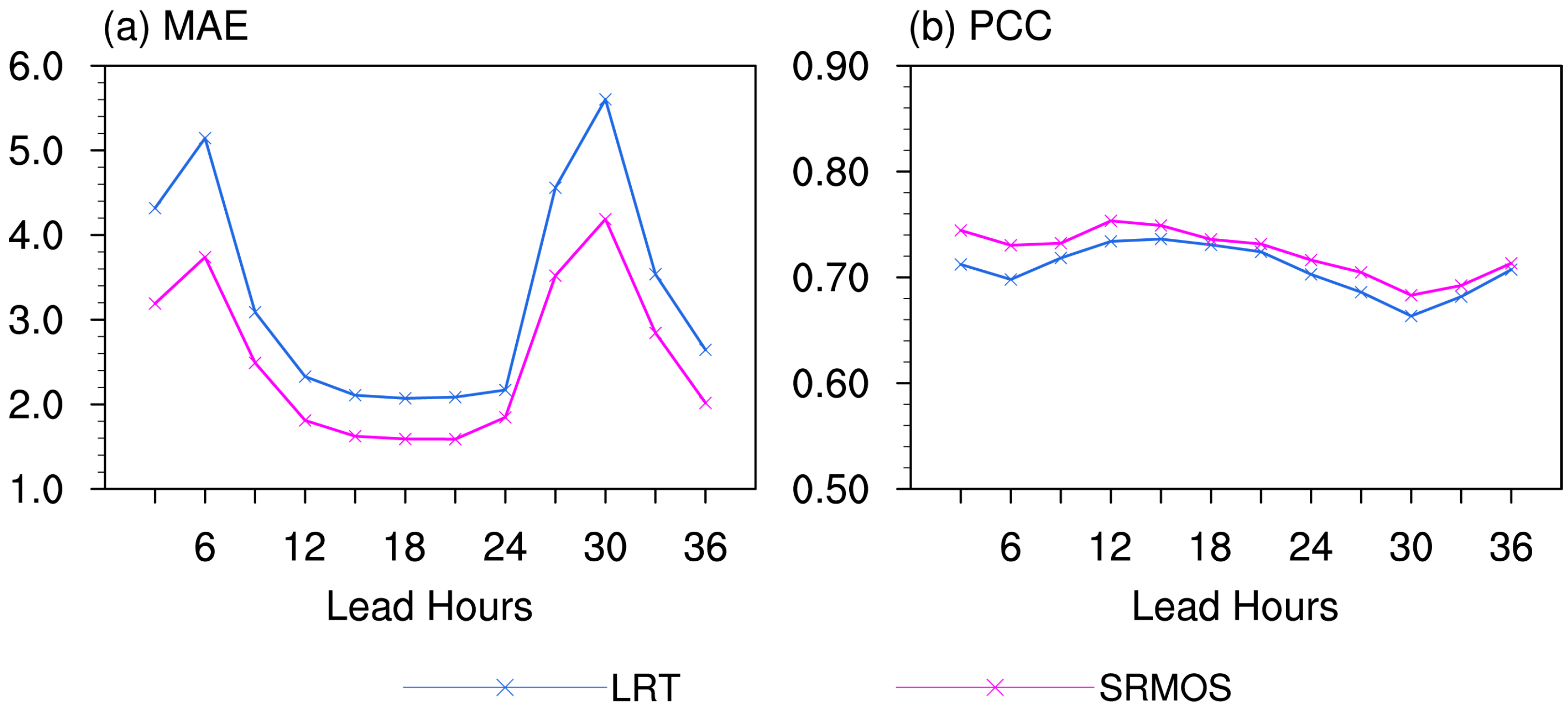
The overall assessments of the multi-variate SRMOS model and the benchmark of the univariate LRT are presented in Figure 3, including the MAE and PCC variations of pavement temperature forecasts at lead times of 3–36 h averaged over the transportation meteorological observation stations along the Jiangsu highways in 2020.
The MAE trends are generally consistent between the two forecast models of pavement temperatures, which show increasing (decreasing) MAE for lead times of 3–6 h and 21–30 h (6–15 h and 30–36 h). At the 3-h lead time, the LRT model has a MAE of 4.3 °C, which then rises to 5.1 °C at the 6-h lead time. It then decreases to a great extent until the lead time of 15 h reaches 2.2 °C and thereafter stabilizes gradually for 9 h. From the lead time of 24 h, the MAE further increases rapidly to the lead time of 30 h, reaches up to 5.6 °C, and afterwards decreases to 2.6 °C at the lead time of 36 h. By contrast, the SRMOS evidently reduces the MAE for all lead times by 0.7–1.6 °C. It is noted that among the lead times of 3–36 h, towards the pavement temperature forecasts with larger biases in LRT, the SRMOS model shows greater magnitudes of effective calibrations. It generally shows a stable capability for improving the forecasting skills of pavement temperatures. Consequently, the SRMOS forecasts are characterized by the largest MAE of 4.0 °C at the 30-h lead time and the lowest of 1.5 °C for lead times of 15–21 h, indicating general superiority to the previous models on pavement temperature forecasts [54,58].
From the perspective of forecasts on spatial distributions of pavement temperatures, the two forecast models display generally similar PCCs. At a lead time of 3 h, the LRT and SRMOS have PCCs of 0.71 and 0.74, respectively. With the increasing lead times, although the models feature overall decreasing PCCs, they remain capable of forecasting the pavement temperature distributions, showing PCCs ranging from 0.66 to 0.75. Furthermore, the results imply higher forecast skills for the SRMOS model than the LRT, which further demonstrate the extensive superiority of the proposed SRMOS model in grasping the spatial distribution of pavement temperature forecasts.
It is worth noting that no matter the simple LRT model or the improved SRMOS models, the lead times of 6 h and 30 h are both characterized by higher forecast errors and lower correlation coefficients, indicating less skillful forecasts of the pavement temperatures at the two lead times than the others. In fact, in the forecast experiments examined here in the manuscript, we take the initialization time of 00:00 UTC, and the lead times of 6 h and 30 h both denote 06:00 UTC, i.e., 14:00 CST (UTC+8). That is, the forecasts at these two lead times almost represent the maximum temperatures during the daytime, while the lead time of 18 h denotes the minimum temperatures during the nighttime. These are consistent with the previous studies revealing more skillful forecasts on the minimum temperatures than the maximums [59,60]. On the one hand, the climatology analysis shows the higher inherent uncertainties (represented by the observational variability without forecast impacts) of the maximum temperature than the minimum, which intends to generate higher biases in forecasts of the maximums [61]. On the other hand, compared with the nighttime with zero solar irradiance, the additional solar radiation in the daytime would increase the net radiation and induce higher biases over the planetary boundary layer in the numerical prediction models [62,63,64]. Combined with the non-perfect physical parameterizations, it results in less skillful forecasts of maximum temperatures than minimums [65,66].

3.2. Details of the Forecast Biases

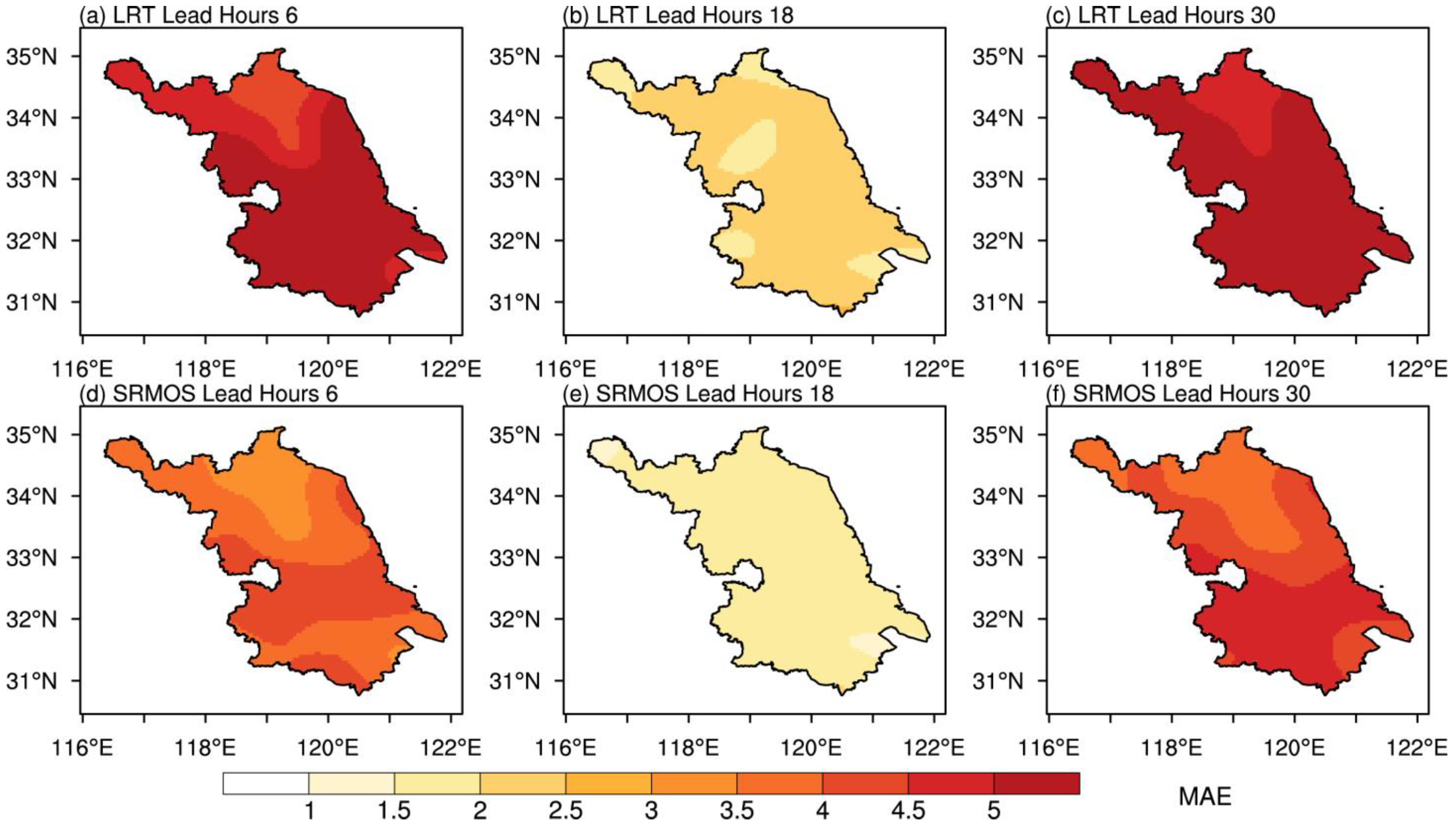
The above section has investigated the general capabilities of the two models of LRT and SRMOS for forecasting pavement temperatures in terms of MAE and PCC. Aiming at more details of the forecast analyses, Figure 4 and Figure 5 present the spatial distributions of pavement temperature forecast MAEs and the corresponding MAESSs, with the lead times of 6 h, 18 h, and 30 h taken as examples. It is noted that to provide more perspicuous and more readable spatial distributions of the forecast assessments, the MAEs and MAESSs at the transportation meteorological observation stations along the highways are interpolated into the whole Jiangsu province.
In terms of the simple LRT model, almost all the areas are characterized by MAEs of greater than 4.0 °C at the lead time of 6 h, and it generally shows an increasing MAE trend from the north to the south. At the lead time of 18 h, the MAEs decrease to ~2.5 °C, distributing evenly across the whole experiment area. When the lead time increases to 30 h, the forecast errors are again increased to a great extent, with the MAEs reaching up to 5.0 °C. By contrast, the multi-factor SRMOS model effectively reduced the errors throughout the whole forecast experiment on the pavement temperature. At the early stage of the 6-h lead time, the MAEs are reduced to less than 4.0 °C, and the temporally averaged MAEs are mainly less than 3.0 °C over the northern part. As for the lead time of 18 h, it shows MAEs ranging from 1.0–2.0 °C over the whole area and generally resembles the evenly distributed features of the LRT model. When the lead time rises to 30 h, the MAE generally shows similar distributions to the lead time of 6 h, i.e., lower MAEs at the north and higher MAEs at the south. However, the magnitudes are definitely higher than the MAEs at the 6-h and 18-h lead times, but still lower than those of the LRT model.
With respect to the forecast improvement features of the SRMOS for LRT, the positive MAESSs denote the consistent and stable calibrations of the SRMOS model. At the lead time of 6 h, the MAESS shows an increasing trend from north to south, indicating that the SRMOS superiority is greater over the southern part of Jiangsu Province. Meanwhile, the MAESSs at the 18-h lead time do not show large spatial differences. Furthermore, for such a lead time with lower forecast biases evenly distributed, the SRMOS remains positive and moderately improving magnitudes to LRT over the whole area, although the MAESSs are generally smaller than those at the 6-h lead time. At the longer lead time of 30 h with larger biases, the MAESSs are predominantly distributed between those of the 6th and 18th lead hours. On the other hand, the spatial distributions indicate that over the areas with larger errors in LRT forecasts, the SRMOS model is characterized by greater improvement magnitudes, while for lower raw errors, it implements relatively fewer improvements based on the LRT results. The considerable calibration capability of the SRMOS model is therefore demonstrated in forecasting pavement temperatures over the Jiangsu highways.
Furthermore, in order to detect the forecast error distributions, Figure 6 exhibits the different proportions of multiple MAE thresholds for the pavement temperature forecasts derived from the LRT and SRMOS models, taking the lead times of 6 h, 12 h, 18 h, 24 h, and 30 h as examples. At the lead time of 6 h, the simple LRT model shows proportions of only ~7% for MAEs of 0–2 °C, and the majority of MAEs are mainly concentrated over 4 °C and even higher than 5 °C. On the other hand, the SRMOS model slightly increases the proportions of 0–2 °C MAEs to ~10% while reducing the larger MAEs to a greater extent and displaying the MAEs concentrating between 3 °C and 5 °C. With the lead times increasing until 18 h, the proportions of smaller (larger) MAEs become larger (smaller). At the 18th lead hour, the LRT shows a ~42% (~54%) proportion of 0–2 °C (2–3 °C) MAE, whereas in the SRMOS model, most MAEs are distributed among 0–2 °C with a proportion of ~91%. Afterwards, the proportions of smaller (larger) MAEs gradually decrease (increase). Moreover, it is notable that for the lead times except 30 h, the MAEs of >5 °C are almost cleared. That is, towards the pavement temperature forecasts, the significant improvements of the SRMOS model are reflected by the notably more concentrated lower biases and the decreasing proportions of larger biases.
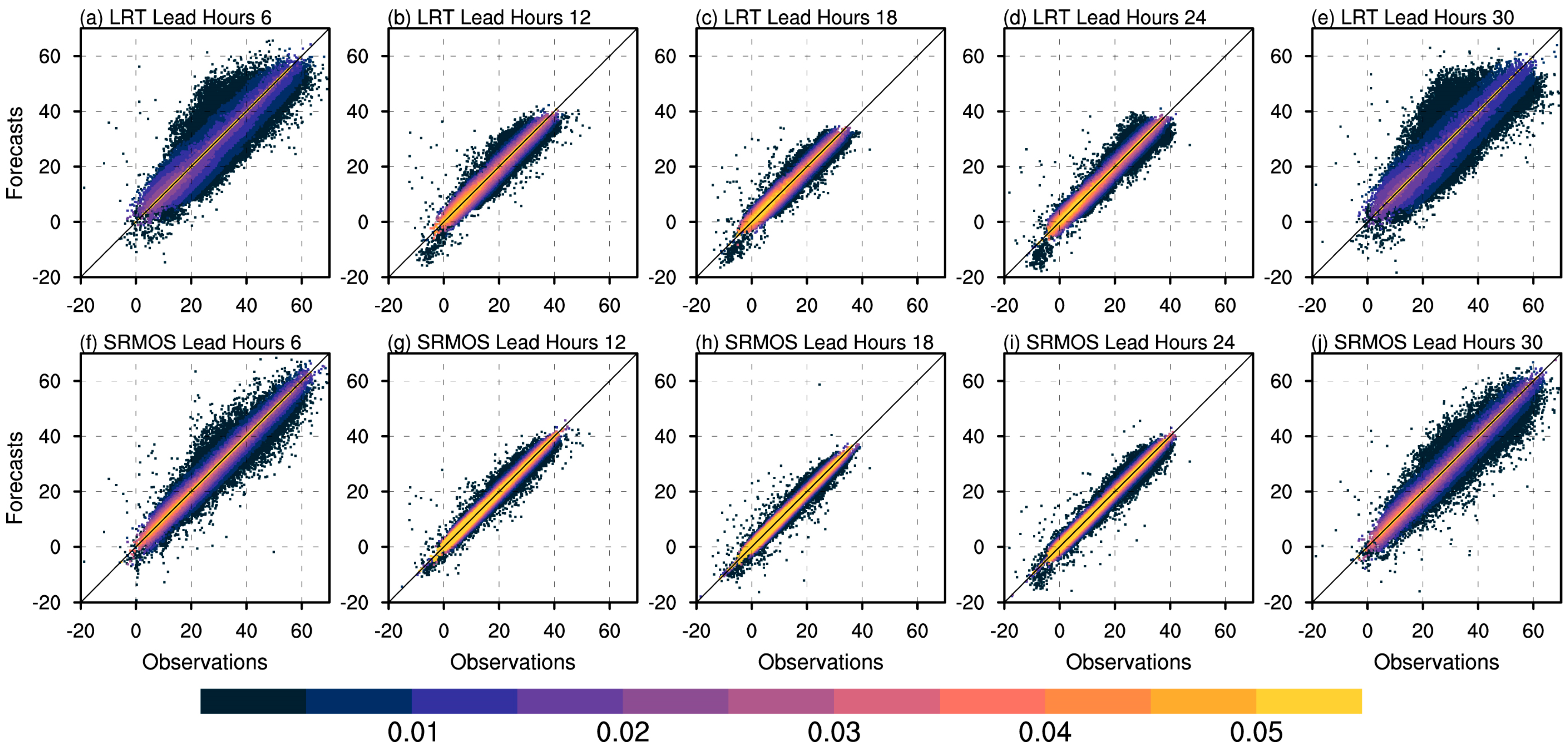
In more detail, Figure 7 displays the corresponding scatter diagram describing the observations (X-axis) and forecasts (Y-axis) of LRT and SRMOS in the forecast experiments of pavement temperatures at multiple lead times. To be noted, the samples from upper left (bottom right) to the diagonal denote warm (cold) biases of the pavement temperature forecasts, and the distance of individual points to the diagonal refers to the deviation of the forecast from observation. In the LRT forecasts, the error distributions are asymmetric, with warm biases occurring more frequently than cold ones. By contrast, the samples become closer and more concentrated around the diagonal in the SRMOS postprocessing output. Even for the extreme cases with samples distributed at the bottom-left and upper-right ends of the sample cluster, the SRMOS is also characterized by considerable improvements over the LRT results. That is, the forecast errors can be sufficiently reduced and become convergent and symmetric to zero after the SRMOS postprocessing, which is particularly evident for the lead times with larger initial biases (e.g., 6 h and 30 h). It further indicates the generally higher skill of the SRMOS model than LRT in predicting pavement temperatures and also implies the potential capability of SRMOS in improving forecast skills for extreme events.

3.3. Predictor Importance Analysis

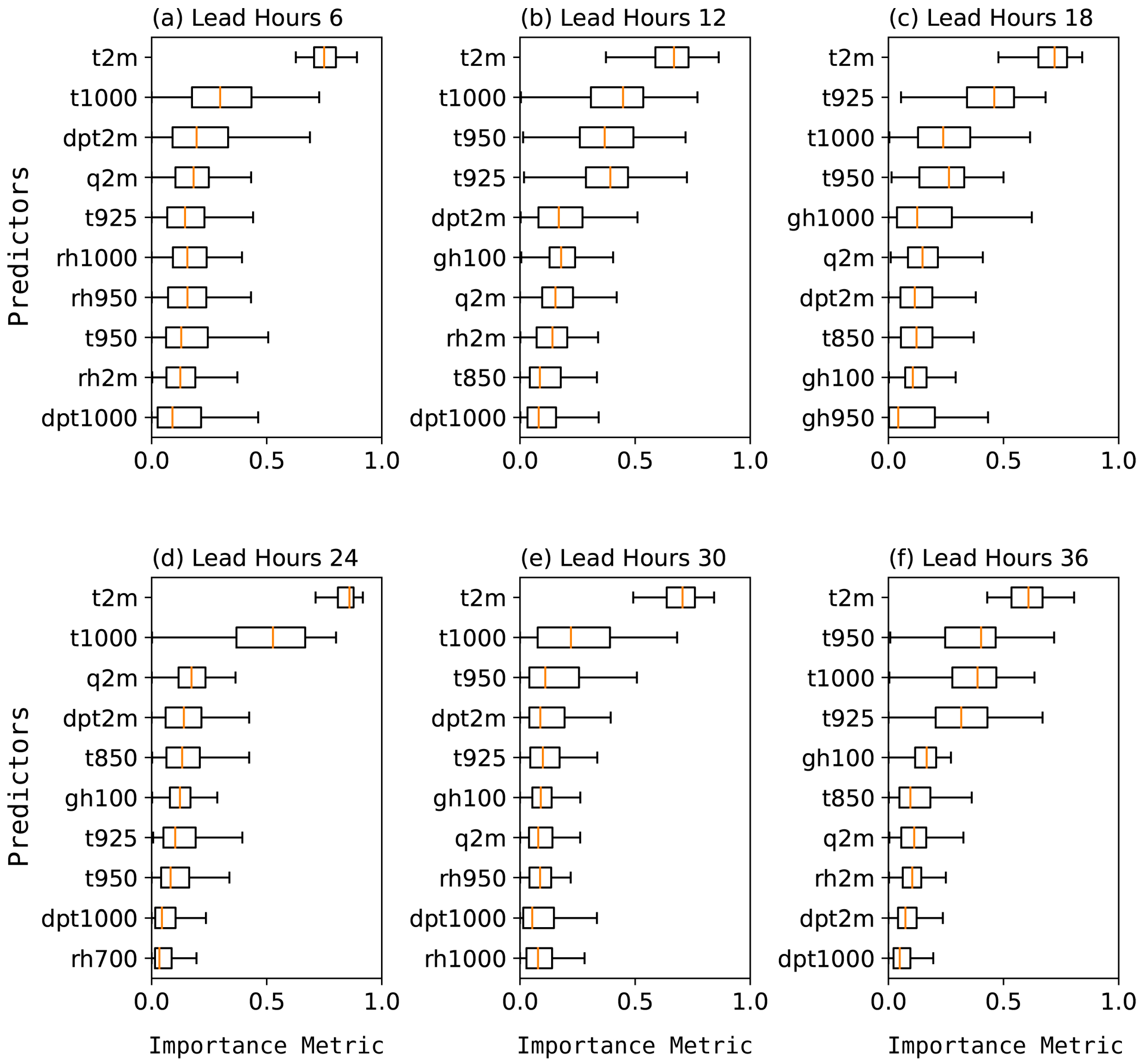
According to the analyzed results on multiple statistics, the SRMOS model has been demonstrated to be effective in pavement temperature forecasts. However, the model has only been a “technical toolbox” until now, and the predictability sources of the model have not yet been revealed. Therefore, to make the model clearer and more explainable, Figure 8 presents the importance metric distributions of the 10 most important predictors employed in the SRMOS model established in the above-analyzed experiments for lead times of 6 h, 12 h, 18 h, 24 h, and 30 h. Associated predictor abbreviations can be referred to in Table 2.
Notably, the predictor’s importance is different for different lead times. According to the boxplot distributions, the importance scores of the individual predictors also maintain a great extent of dispersion among the samples. Detailed analyses show that the key factors could generally be classified into three categories associated with temperature, moisture, and larger-scale background at multiple levels, respectively.
Specifically, the surface air temperature at the 2-m level (t2m) always remains the most critical predictor at all lead times. The importance scores of t2m reach greater than 0.8 at multiple lead times, which is much higher than those of the other predictors. The following several important factors also focus on the temperatures at higher levels, such as 1000 hPa and 925 hPa. That is, the pavement temperature forecast skills of the SRMOS model could preliminarily be attributed to the air temperature forecasts in the numerical prediction model.
Besides, considering that the dew point temperatures are also an effective factor featuring the comprehensive conditions of temperature and moisture and combining the importance distributions of dew point temperature (dpt), specific humidity (q), and relative humidity (rh), the moisture-related predictors, particularly at the lower levels, also play important roles in the pavement temperature forecasts. On average, they count each importance metric at 0.1–0.2, although the scores are slightly decreased with the increasing lead times. These demonstrate that, following air temperatures, moisture factors are the second-most important predictors in the SRMOS model for pavement temperature forecasts.
Moreover, it is also noted that the larger-scale backgrounds, such as geopotential height (gh), also make certain sense in the model construction. At the early stage of the forecast, it has not yet been included in the top 10 predictors at the lead time of 6 h (Figure 8a). Afterwards, the associated predictors are generally characterized by importance scores of ~0.1, accompanied by an overall increasing trend at lead times from 12 h to 36 h. It might be associated with the consistently promising forecasts of larger-scale backgrounds in the numerical prediction models at the short-term timescale, while the specific parameters (e.g., precipitation, wind, etc.) could not always be represented so stably or sufficiently [67,68].
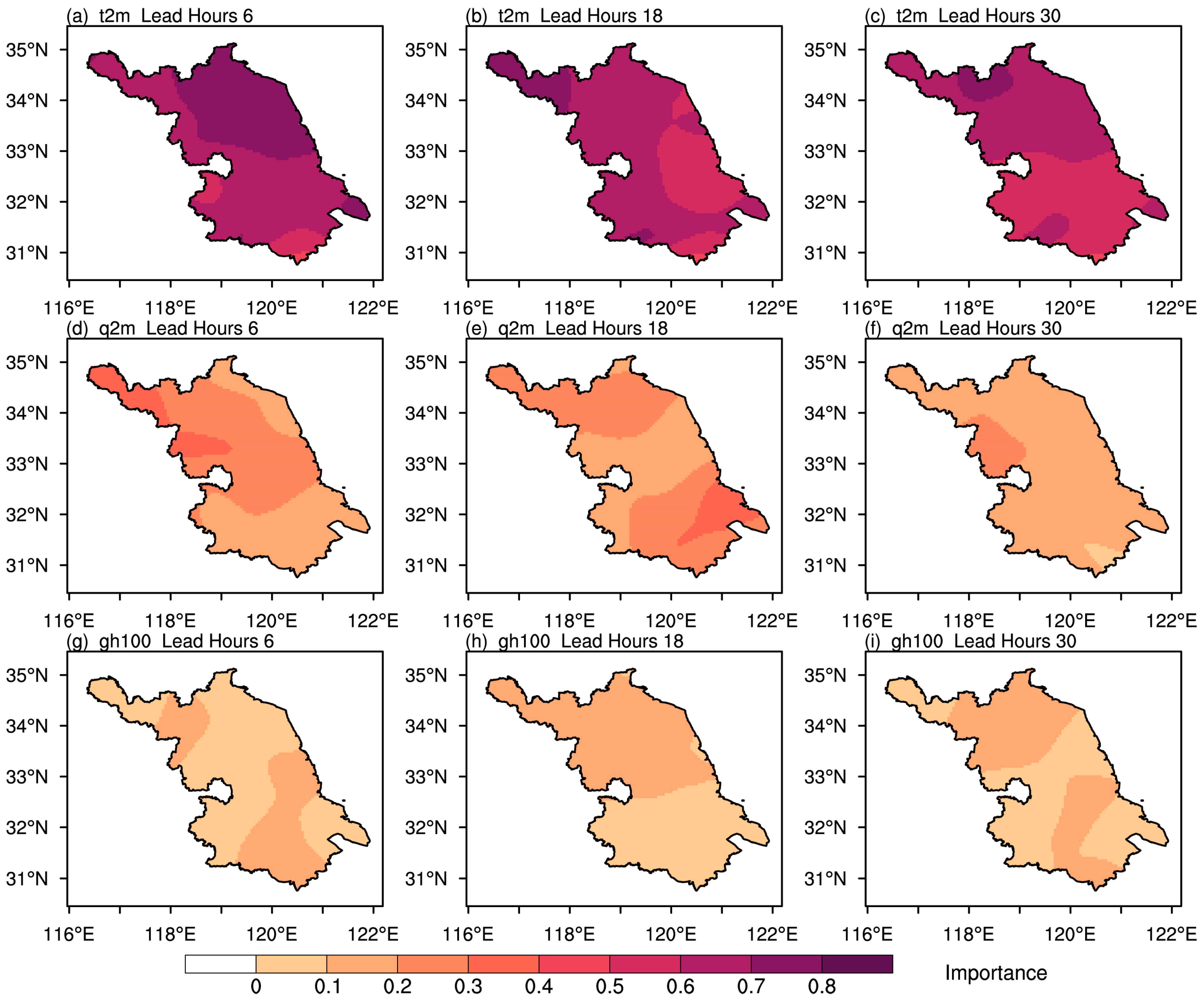
In summary, temperature, moisture, and larger-scale background are basically the key predictors in the SRMOS model of pavement temperature forecasts. Figure 9 further describes the spatial distributions of the typical predictor importance metrics for lead times of 6 h, 18 h, and 30 h. Based on analyses of Figure 8, the predictors of t2m, q2m, and gh100 are determined to express aspects of temperature, moisture, and larger-scale background, respectively.
The importance metric distributions of t2m correspond well to its remarkable and largest contributions to the model forecast skills shown in the boxplots. With the growing lead times, the importance slightly decreases by ~0.1 for every lead time interval of 6 h. From the perspective of spatial distribution, the t2m importance generally shows a decreasing trend from north to south. It indicates strong consistency with the SRMOS forecast skill distributions, which are higher in the north and lower in the south (Figure 4). That is, in the SRMOS model, the higher predictor importance of t2m always corresponds to more skillful pavement temperature forecasts. On the other hand, the forecast skills of pavement temperature are also jointly impacted by forecasts of the air temperature itself and the other predictors. As for the moisture-associated and larger-scale background predictors of q2m and gh100, they both do not show significant regional characteristics or consistently changing distributions. Meanwhile, q2m features greater importance than gh100 throughout the whole lead period in the pavement temperature forecast experiments.

4. Conclusions

In this study, we propose a pavement temperature forecast model based on stepwise regression—model output statistics (SRMOS) at the short-term timescale, using the highways in Jiangsu, China, as examples. The linear regression based on the surface air temperature (LRT) model is also conducted in parallel as a benchmark. The conversions from the numerical prediction model outputs to the pavement temperature forecasts are therefore effectively realized. The conclusions obtained are summarized as follows:
The SRMOS model shows effective calibrations towards the pavement temperature forecasts based on the LRT model. The mean absolute errors are generally reduced by 0.7–1.6 °C, with greater magnitudes for larger biases in the LRT model. At lead times of 15–21 h, the biases are only ~1.5 °C for the proposed SRMOS model. Both the LRT and SRMOS models are capable of well predicting the spatial distributions of the pavement temperatures, although they both exhibit decreasing trends for pattern correlation coefficients. The SRMOS model slightly outperforms the LRT in terms of spatial representation. It is worth noting that the forecast performance for maximum daytime temperatures is inferior to that for minimum nighttime temperatures. The discrepancy could be attributed to the higher inherent uncertainties of maximum temperatures and the imperfect physical parameterizations of additional solar radiation during the daytime.
No matter whether the simple LRT model or the SRMOS model is used, they generally indicate increasing forecast biases from north to south. The SRMOS model exhibits greater superiority in the southern part of Jiangsu Province, where initial LRT biases are larger. That is, the SRMOS model is characterized by notably more concentrated lower biases and decreasing proportions of larger biases. It further demonstrates the overall higher skill of the SRMOS model compared to the LRT model in predicting pavement temperatures and also suggests the potential capability of SRMOS in improving forecast skills for extreme events.
Predictor importance analysis shows that temperature, moisture, and larger-scale background are basically the key predictors in the SRMOS model, of which the air temperatures are the most crucial factors in the model construction of the pavement temperature forecasts. Although the larger-scale circulation backgrounds are generally characterized by lower importance metrics, they are accompanied by an overall increasing trend with increasing lead times, which might be associated with the consistently promising forecasts of larger-scale backgrounds in numerical prediction models at the short-term timescale.

5. Discussion

Accurate pavement temperature forecasts are essential for various applications, such as transportation planning, road maintenance, and weather impact assessments, which help optimize road treatments, prevent accidents, and enhance overall infrastructure safety. The current study presents the stepwise regression—model output statistics (SRMOS) model for pavement temperature forecasts based on the numerical prediction model PWAFS. Although the model itself is still characterized by specific forecast biases according to the examinations conducted in Jiangsu Province, China, it could be considered able to well forecast pavement temperatures and has been demonstrated to be effective in practical applications.
It is important to note that the study only utilizes and tests one numerical prediction model, i.e., the Jiangsu regionally operated forecast model PWAFS. This might introduce certain uncertainties and biases due to the model’s properties. Since the SRMOS model is constructed based on dynamical-model training data and observations, the selected predictors may differ across different models. Therefore, it is necessary to attempt more numerical prediction models to assess their applicability and capability in transportation meteorological forecasts, particularly for pavement temperatures. Meanwhile, given the multi-model outputs, the ensemble techniques, which have been successfully utilized in weather forecast scopes [69], are worth examining in transportation meteorological forecasts to exploit the benefits of multiple models.
Furthermore, advanced statistical postprocessing procedures, including state-of-the-art machine learning methods, should be employed to achieve transportation meteorological early warnings and forecasts and to reduce the biases of numerical prediction models [70,71]. Probability forecast systems can also be developed to provide more detailed information from multi-model ensembles [72]. Moreover, bias decompositions are to be investigated to reveal more comprehensive insights into the behavior of multiple forecast models for pavement temperatures and other factors [73], which would also aid in the intelligent establishment of associated forecast models.
Reliable transportation meteorological observations also play crucial roles in ensuring refined and accurate forecasts of transportation meteorological factors such as pavement temperature. For instance, remote sensing measurements feature the advantages of their high versatility, scalability, sensitivity, reliability, and stability, making them helpful for not only more accurate forecasts but also investigations on associated physical mechanisms [74]. These should never be overlooked in either the business forecasts or operational services of the transportation or meteorology agencies [75]. Furthermore, more reasonable planning and layout of future multi-source transportation meteorological observation networks would also benefit from the integration of remote sensing observations [76].

Author Contributions

Conceptualization, S.Z. and H.W. (Hongbin Wang); methodology, Y.L. and L.Z. (Linyi Zhou); validation, C.Z., D.L. and L.Z. (Ling Zhang); formal analysis, F.D.; investigation, Y.F.; resources, H.W. (Hong Wu); data curation, T.Y. and D.K.; writing—original draft preparation, S.Z.; writing—review and editing, S.Z., H.W. (Hongbin Wang), Y.F. and L.Z. (Ling Zhang). All authors have read and agreed to the published version of the manuscript.

Funding

This research was jointly funded by the Basic Research Fund of CAMS (2022Y027), the Joint Fund for Innovation and Development of the Natural Science Foundation of Hubei Province (2022CFD132), the National Natural Science Foundation of China (42205162), the Innovation and Development Project of China Meteorological Administration (CXFZ2023J022), and the Provincial and Municipal Joint Fund Project of Guizhou Province Meteorological Bureau “Research on AI-based intelligent weather monitoring and dispatching technology”.

Data Availability Statement

The data presented in this study are available on request from the corresponding author.

Acknowledgments

The authors are grateful to Jiangsu Meteorological Bureau, China, and Jintan Field Scientific Experiment Base for Transportation Meteorology of China Meteorological Administration for the data and resources. The constructive comments of the anonymous reviewers are acknowledged. We also thank Weiguang Liu for extensive discussions on the numerical weather prediction model PWAFS.

Conflicts of Interest

The authors declare no conflict of interest.

References

  1. Zhu, S.P.; Ge, F.; Fan, Y.; Zhang, L.; Sielmann, F.; Fraedrich, K.; Zhi, X.F. Conspicuous temperature extremes over Southeast Asia: Seasonal variations under 1.5 degrees C and 2 degrees C global warming. Clim. Change 2020, 160, 343–360. [Google Scholar] [CrossRef]
  2. Yan, Y.; Wang, H.; Li, G.; Xia, J.; Ge, F.; Zeng, Q.; Ren, X.; Tan, L. Projection of Future Extreme Precipitation in China Based on the CMIP6 from a Machine Learning Perspective. Remote Sens. 2022, 14, 4033. [Google Scholar] [CrossRef]
  3. You, Q.L.; Chen, D.L.; Wu, F.Y.; Pepin, N.; Cai, Z.Y.; Ahrens, B.; Jiang, Z.H.; Wu, Z.W.; Kang, S.C.; AghaKouchak, A. Elevation dependent warming over the Tibetan Plateau: Patterns, mechanisms and perspectives. Earth Sci. Rev. 2020, 210, 103349. [Google Scholar] [CrossRef]
  4. Sun, X.R.; Ge, F.; Fan, Y.; Zhu, S.P.; Chen, Q.L. Will population exposure to heat extremes intensify over Southeast Asia in a warmer world? Environ. Res. Lett. 2022, 17, 044006. [Google Scholar] [CrossRef]
  5. Zhu, S.P.; Yang, H.D.; Liu, D.Y.; Wang, H.B.; Zhou, L.Y.; Zhu, C.Y.; Zu, F.; Wu, H.; Lyu, Y.; Xia, Y.; et al. Observations and Forecasts of Urban Transportation Meteorology in China: A Review. Atmosphere 2022, 13, 1823. [Google Scholar] [CrossRef]
  6. Zhu, S.P.; Zhi, X.F.; Ge, F.; Fan, Y.; Zhang, L.; Gao, J.Y. Subseasonal Forecast of Surface Air Temperature Using Superensemble Approaches: Experiments over Northeast Asia for 2018. Weather Forecast. 2021, 36, 39–51. [Google Scholar] [CrossRef]
  7. Pisano, P.; Goodwin, L.; Stern, A. Surface transportation safety and operations: The impacts of weather within the context of climate change. In Proceedings of the Potential Impacts of Climate Change on Transportation Workshop, US Department of Transportation: Centre for Climate Change and Environmental Forecasting, Washington, DC, USA, 1–2 October 2002. [Google Scholar]
  8. Kim, Y.-J.; Kim, B.-J.; Shin, Y.-S.; Kim, H.-W.; Kim, G.-T.; Kim, S.-J. A case study of environmental characteristics on urban road-surface and air temperatures during heat-wave days in Seoul. Atmos. Ocean. Sci. Lett. 2019, 12, 261–269. [Google Scholar] [CrossRef] [Green Version]
  9. Androjić, I.; Marović, I. Analysis of influential factors on heat accumulation in structural elements of road underpasses. Sol. Energy 2017, 155, 25–34. [Google Scholar] [CrossRef]
  10. Dey, K.C.; Mishra, A.; Chowdhury, M. Potential of Intelligent Transportation Systems in Mitigating Adverse Weather Impacts on Road Mobility: A Review. IEEE Trans. Intell. Transp. Syst. 2015, 16, 1107–1119. [Google Scholar] [CrossRef]
  11. Douglas, E.; Jacobs, J.; Hayhoe, K.; Silka, L.; Daniel, J.; Collins, M.; Alipour, A.; Anderson, B.; Hebson, C.; Mecray, E.; et al. Progress and Challenges in Incorporating Climate Change Information into Transportation Research and Design. J. Infrastruct. Syst. 2017, 23, 9. [Google Scholar] [CrossRef] [Green Version]
  12. Crevier, L.-P.; Delage, Y. METRo: A New Model for Road-Condition Forecasting in Canada. J. Appl. Meteorol. 2001, 40, 2026–2037. [Google Scholar] [CrossRef]
  13. Chen, J.; Wang, H.; Xie, P. Pavement temperature prediction: Theoretical models and critical affecting factors. Appl. Therm. Eng. 2019, 158, 113755. [Google Scholar] [CrossRef]
  14. Adwan, I.; Milad, A.; Memon, Z.A.; Widyatmoko, I.; Ahmat Zanuri, N.; Memon, N.A.; Yusoff, N.I.M. Asphalt Pavement Temperature Prediction Models: A Review. Appl. Sci. 2021, 11, 3794. [Google Scholar]
  15. Herb, W.; Velasquez, R.; Stefan, H.; Marasteanu, M.O.; Clyne, T. Simulation and Characterization of Asphalt Pavement Temperatures. Road Mater. Pavement Des. 2009, 10, 233–247. [Google Scholar] [CrossRef] [Green Version]
  16. Chao, J.; Jinxi, Z. Prediction Model for Asphalt Pavement Temperature in High-Temperature Season in Beijing. Adv. Civ. Eng. 2018, 2018, 1837952. [Google Scholar] [CrossRef] [Green Version]
  17. Wang, T.-h.; Su, L.-j.; Zhai, J.-y. A case study on diurnal and seasonal variation in pavement temperature. Int. J. Pavement Eng. 2014, 15, 402–408. [Google Scholar] [CrossRef]
  18. Resler, J.; Krč, P.; Belda, M.; Juruš, P.; Benešová, N.; Lopata, J.; Vlček, O.; Damašková, D.; Eben, K.; Derbek, P.; et al. PALM-USM v1.0: A new urban surface model integrated into the PALM large-eddy simulation model. Geosci. Model Dev. 2017, 10, 3635–3659. [Google Scholar] [CrossRef] [Green Version]
  19. Milad, A.A.; Adwan, I.; Majeed, S.A.; Memon, Z.A.; Bilema, M.; Omar, H.A.; Abdolrasol, M.G.M.; Usman, A.; Yusoff, N.I.M. Development of a Hybrid Machine Learning Model for Asphalt Pavement Temperature Prediction. IEEE Access 2021, 9, 158041–158056. [Google Scholar] [CrossRef]
  20. Tabrizi, S.E.; Xiao, K.; Van Griensven Thé, J.; Saad, M.; Farghaly, H.; Yang, S.X.; Gharabaghi, B. Hourly road pavement surface temperature forecasting using deep learning models. J. Hydrol. 2021, 603, 126877. [Google Scholar] [CrossRef]
  21. Wilks, D.S.; Vannitsem, S. Chapter 1—Uncertain Forecasts From Deterministic Dynamics. In Statistical Postprocessing of Ensemble Forecasts; Vannitsem, S., Wilks, D.S., Messner, J.W., Eds.; Elsevier: Amsterdam, The Netherlands, 2018; pp. 1–13. [Google Scholar] [CrossRef]
  22. Skamarock, C.; Klemp, B.; Dudhia, J.; Gill, O.; Barker, D.M.; Duda, G.; Huang, X.; Wang, W.; Powers, G. A Description of the Advanced Research WRF Version 3. NCAR Tech. Note 2008, 475, 113. [Google Scholar]
  23. Zhang, L.; Song, L.X.; Zhu, S.P.; Guo, Z.; Wang, H.B.; Zhou, L.Y.; Chen, C.H.; Zhi, X.F. Forecasts of the Warm-Sector Heavy Rainfall With a Warm Shear Pattern Over Coastal Areas of the Yangtze-Huaihe River in a Regional Business Forecast Model. Front. Earth Sci. 2022, 10, 938336. [Google Scholar] [CrossRef]
  24. Lorenz, E.N. Deterministic Nonperiodic Flow. J. Atmos. Sci. 1963, 20, 130–141. [Google Scholar] [CrossRef]
  25. LORENZ, E.N. The predictability of a flow which possesses many scales of motion. Tellus 1969, 21, 289–307. [Google Scholar] [CrossRef]
  26. Slingo, J.; Palmer, T. Uncertainty in weather and climate prediction. Philos. Trans. R. Soc. A-Math. Phys. Eng. Sci. 2011, 369, 4751–4767. [Google Scholar] [CrossRef]
  27. Zhu, Y.J.; Zhou, X.Q.; Pena, M.; Li, W.; Melhauser, C.; Hou, D.C. Impact of Sea Surface Temperature Forcing on Weeks 3 and 4 Forecast Skill in the NCEP Global Ensemble Forecasting System. Weather Forecast. 2017, 32, 2159–2174. [Google Scholar] [CrossRef]
  28. Krishnamurti, T.N.; Kishtawal, C.M.; Zhang, Z.; LaRow, T.; Bachiochi, D.; Williford, E.; Gadgil, S.; Surendran, S. Multimodel Ensemble Forecasts for Weather and Seasonal Climate. J. Clim. 2000, 13, 4196–4216. [Google Scholar] [CrossRef]
  29. Vannitsem, S.; Bremnes, J.B.; Demaeyer, J.; Evans, G.R.; Flowerdew, J.; Hemri, S.; Lerch, S.; Roberts, N.; Theis, S.; Atencia, A.; et al. Statistical Postprocessing for Weather Forecasts: Review, Challenges, and Avenues in a Big Data World. Bull. Amer. Meteorol. Soc. 2021, 102, E681–E699. [Google Scholar] [CrossRef]
  30. Hamill, T.M. Chapter 7—Practical Aspects of Statistical Postprocessing. In Statistical Postprocessing of Ensemble Forecasts; Vannitsem, S., Wilks, D.S., Messner, J.W., Eds.; Elsevier: Amsterdam, The Netherlands, 2018; pp. 187–217. [Google Scholar] [CrossRef]
  31. Feng, J.; Zhang, J.; Toth, Z.; Peña, M.; Ravela, S. A New Measure of Ensemble Central Tendency. Weather Forecast. 2020, 35, 879–889. [Google Scholar] [CrossRef]
  32. Klein, W.H.; Lewis, B.M.; Enger, I. Objective prediction of five-day mean temperatures during winter. J. Atmos. Sci. 1959, 16, 672–682. [Google Scholar] [CrossRef]
  33. Glahn, H.R.; Lowry, D.A. The Use of Model Output Statistics (MOS) in Objective Weather Forecasting. J. Appl. Meteorol. Climatol. 1972, 11, 1203–1211. [Google Scholar] [CrossRef]
  34. Vannitsem, S. Dynamical Properties of MOS Forecasts: Analysis of the ECMWF Operational Forecasting System. Weather Forecast. 2008, 23, 1032–1043. [Google Scholar] [CrossRef]
  35. Li, W.T.; Duan, Q.Y.; Wang, Q.J. Factors Influencing the Performance of Regression-Based Statistical Postprocessing Models for Short-Term Precipitation Forecasts. Weather Forecast. 2019, 34, 2067–2084. [Google Scholar] [CrossRef]
  36. Sokol, Z.; Bliznak, V.; Sedlak, P.; Zacharov, P.; Pesice, P.; Skuthan, M. Ensemble forecasts of road surface temperatures. Atmos. Res. 2017, 187, 33–41. [Google Scholar] [CrossRef]
  37. Yang, Y.; Turner, R.; Carey-Smith, T.; Uddstrom, M. A comparison of three model output statistics approaches for the bias correction of simulated soil moisture. Meteorol. Appl. 2020, 27, 15. [Google Scholar] [CrossRef]
  38. Pinson, P.; Messner, J.W. Chapter 9—Application of Postprocessing for Renewable Energy. In Statistical Postprocessing of Ensemble Forecasts; Vannitsem, S., Wilks, D.S., Messner, J.W., Eds.; Elsevier: Amsterdam, The Netherlands, 2018; pp. 241–266. [Google Scholar] [CrossRef]
  39. Li, X.; Zeng, M.; Wang, Y.; Wang, W.; Wu, H.; Mei, H. Evaluation of two momentum control variable schemes and their impact on the variational assimilation of radarwind data: Case study of a squall line. Adv. Atmos. Sci. 2016, 33, 1143–1157. [Google Scholar] [CrossRef]
  40. Li, X.; Zou, X.; Zeng, M. An Alternative Bias Correction Scheme for CrIS Data Assimilation in a Regional Model. Mon. Weather Rev. 2019, 147, 809–839. [Google Scholar] [CrossRef]
  41. Song-You, H.; Jeong-Ock Jade, L. The WRF Single-Moment 6-Class Microphysics Scheme (WSM6). Asia-Pac. J. Atmos. Sci. 2006, 42, 129–151. [Google Scholar]
  42. Monin, A.S.; Obukhov, A.M. Basic laws of turbulent mixing in the surface layer of the atmosphere. Tr. Akad. Nauk SSSR Geophiz. Inst. 1954, 24, 163–187. [Google Scholar]
  43. Chen, F.; Dudhia, J. Coupling an Advanced Land Surface–Hydrology Model with the Penn State–NCAR MM5 Modeling System. Part I: Model Implementation and Sensitivity. Mon. Weather Rev. 2001, 129, 569–585. [Google Scholar] [CrossRef]
  44. Hong, S.-Y.; Noh, Y.; Dudhia, J. A New Vertical Diffusion Package with an Explicit Treatment of Entrainment Processes. Mon. Weather Rev. 2006, 134, 2318–2341. [Google Scholar] [CrossRef] [Green Version]
  45. Mlawer, E.J.; Taubman, S.J.; Brown, P.D.; Iacono, M.J.; Clough, S.A. Radiative transfer for inhomogeneous atmospheres: RRTM, a validated correlated-k model for the longwave. J. Geophys. Res. Atmos. 1997, 102, 16663–16682. [Google Scholar] [CrossRef] [Green Version]
  46. Dudhia, J. Numerical Study of Convection Observed during the Winter Monsoon Experiment Using a Mesoscale Two-Dimensional Model. J. Atmos. Sci. 1989, 46, 3077–3107. [Google Scholar] [CrossRef]
  47. Kain, J.S.; Fritsch, J.M. The role of the convective “trigger function” in numerical forecasts of mesoscale convective systems. Meteorol. Atmos. Phys. 1992, 49, 93–106. [Google Scholar] [CrossRef]
  48. Kain, J.S. The Kain–Fritsch Convective Parameterization: An Update. J. Appl. Meteorol. 2004, 43, 170–181. [Google Scholar] [CrossRef]
  49. Ewan, L.; Al-Kaisy, A.; Veneziano, D. Remote Sensing of Weather and Road Surface Conditions:Is Technology Mature for Reliable Intelligent Transportation Systems Applications? Transp. Res. Rec. 2013, 2329, 8–16. [Google Scholar] [CrossRef] [Green Version]
  50. Navalgund, R.R.; Jayaraman, V.; Roy, P.S. Remote sensing applications: An overview. Curr. Sci. 2007, 93, 1747–1766. [Google Scholar]
  51. Friederichs, P.; Wahl, S.; Buschow, S. Chapter 5—Postprocessing for Extreme Events. In Statistical Postprocessing of Ensemble Forecasts; Vannitsem, S., Wilks, D.S., Messner, J.W., Eds.; Elsevier: Amsterdam, The Netherlands, 2018; pp. 127–154. [Google Scholar] [CrossRef]
  52. Gao, L.; Schulz, K.; Bernhardt, M. Statistical Downscaling of ERA-Interim Forecast Precipitation Data in Complex Terrain Using LASSO Algorithm. Adv. Meteorol. 2014, 2014, 472741. [Google Scholar] [CrossRef] [Green Version]
  53. Hu, X.; Wang, M.; Liu, K.; Gong, D.; Kantz, H. Using Climate Factors to Estimate Flood Economic Loss Risk. Int. J. Disaster Risk Sci. 2021, 12, 731–744. [Google Scholar] [CrossRef]
  54. Feng, L.; Wang, X.; He, X.; Gao, J. Fine forecast of high road temperature along jiangsu highways based on INCA system and METRo model. J. Appl. Meteorol. Sci. 2017, 28, 109–118. [Google Scholar]
  55. Zhang, H.B.; Zhi, X.F.; Chen, J.; Wang, Y.N.; Wang, Y. Study of the modification of multi-model ensemble schemes for tropical cyclone forecasts. J. Trop. Meteorol. 2015, 21, 389–399. [Google Scholar]
  56. Breiman, L. Random Forests. Mach. Learn. 2001, 45, 5–32. [Google Scholar] [CrossRef] [Green Version]
  57. Kuhn, M.; Johnson, K. Measuring Predictor Importance. In Applied Predictive Modeling; Kuhn, M., Johnson, K., Eds.; Springer: New York, NY, USA, 2013; pp. 463–485. [Google Scholar] [CrossRef]
  58. Yan, X.; Wang, X.; Da, X.; Zhao, F.; Niu, X. Variation Characteristics of Expressway Pavement Temperature and Forecast Model in Mountainous Area of Gansu. J. Arid. Meteorol. 2018, 36, 864–872. [Google Scholar]
  59. Lyu, Y.; Zhi, X.F.; Zhu, S.P.; Fan, Y.; Pan, M.T. Statistical Calibrations of Surface Air Temperature Forecasts over East Asia Using Pattern Projection Methods. Weather. Forecast. 2021, 36, 1661–1674. [Google Scholar] [CrossRef]
  60. Zhu, S.; Zhang, L.; Jiang, H.; Lyu, Y.; Fan, Y.; Guo, Z.; Zhi, X. Pattern projection calibrations on subseasonal forecasts of surface air temperature over East Asia. Weather. Forecast. 2023, 38, 865–878. [Google Scholar] [CrossRef]
  61. Najafi, R.; Kermani, M.R.H. Uncertainty Modeling of Statistical Downscaling to Assess Climate Change Impacts on Temperature and Precipitation. Water Resour. Manag. 2017, 31, 1843–1858. [Google Scholar] [CrossRef]
  62. Zamora, R.J.; Dutton, E.G.; Trainer, M.; McKeen, S.A.; Wilczak, J.M.; Hou, Y.T. The accuracy of solar irradiance calculations used in mesoscale numerical weather prediction. Mon. Weather Rev. 2005, 133, 783–792. [Google Scholar] [CrossRef]
  63. Yang, D.Z.; Jirutitijaroen, P.; Walsh, W.M. Hourly solar irradiance time series forecasting using cloud cover index. Sol. Energy 2012, 86, 3531–3543. [Google Scholar] [CrossRef]
  64. Hannak, L.; Knippertz, P.; Fink, A.H.; Kniffka, A.; Pante, G. Why Do Global Climate Models Struggle to Represent Low-Level Clouds in the West African Summer Monsoon? J. Clim. 2017, 30, 1665–1687. [Google Scholar] [CrossRef]
  65. Phakula, S.; Landman, W.A.; Engelbrecht, C.J.; Makgoale, T. Forecast Skill of Minimum and Maximum Temperatures on Subseasonal-to-Seasonal Timescales Over South Africa. Earth Space Sci. 2020, 7, 11. [Google Scholar] [CrossRef] [Green Version]
  66. Srivastava, P.; Sharan, M.; Kumar, M. A note on surface layer parameterizations in the weather research and forecast model. Dyn. Atmos. Oceans 2021, 96, 10. [Google Scholar] [CrossRef]
  67. Hamill, T.M.; Whitaker, J.S. Ensemble Calibration of 500-hPa Geopotential Height and 850-hPa and 2-m Temperatures Using Reforecasts. Mon. Weather Rev. 2007, 135, 3273–3280. [Google Scholar] [CrossRef] [Green Version]
  68. Zhi, X.; Qi, H.; Bai, Y.; Lin, C. A comparison of three kinds of multimodel ensemble forecast techniques based on the TIGGE data. Acta Meteorol. Sin. 2012, 26, 41–51. [Google Scholar] [CrossRef]
  69. Ji, L.; Zhi, X.; Schalge, B.; Stephan, K.; Wu, Z.; Wu, C.; Simmer, C.; Zhu, S. Dynamic downscaling ensemble forecast of an extreme rainstorm event in South China by COSMO EPS. Front. Earth Sci. 2022, 10, 969742. [Google Scholar] [CrossRef]
  70. Zhu, Y.; Zhi, X.; Lyu, Y.; Zhu, S.; Tong, H.; Mamtimin, A.; Zhang, H.; Huo, W. Forecast calibrations of surface air temperature over Xinjiang based on U-net neural network. Front. Environ. Sci. 2022, 10, 11321. [Google Scholar] [CrossRef]
  71. Zhang, J.; Feng, J.; Li, H.; Zhu, Y.; Zhi, X.; Zhang, F. Unified Ensemble Mean Forecasting of Tropical Cyclones Based on the Feature-Oriented Mean Method. Weather. Forecast. 2021, 36, 1945–1959. [Google Scholar] [CrossRef]
  72. Ji, L.; Zhi, X.; Zhu, S.; Fraedrich, K. Probabilistic Precipitation Forecasting over East Asia Using Bayesian Model Averaging. Weather. Forecast. 2019, 34, 377–392. [Google Scholar] [CrossRef]
  73. Lyu, Y.; Zhi, X.; Wu, H.; Zhou, H.; Kong, D.; Zhu, S.; Zhang, Y.; Hao, C. Analyses on the Multimodel Wind Forecasts and Error Decompositions over North China. Atmosphere 2022, 13, 1652. [Google Scholar]
  74. Schnebele, E.; Tanyu, B.F.; Cervone, G.; Waters, N. Review of remote sensing methodologies for pavement management and assessment. Eur. Transp. Res. Rev. 2015, 7, 7. [Google Scholar] [CrossRef] [Green Version]
  75. Capozzi, V.; Mazzarella, V.; Vivo, C.D.; Annella, C.; Greco, A.; Fusco, G.; Budillon, G. A Network of X-Band Meteorological Radars to Support the Motorway System (Campania Region Meteorological Radar Network Project). Remote Sens. 2022, 14, 2221. [Google Scholar] [CrossRef]
  76. Song, Y.; Wright, G.; Wu, P.; Thatcher, D.; McHugh, T.; Li, Q.; Li, S.J.; Wang, X. Segment-Based Spatial Analysis for Assessing Road Infrastructure Performance Using Monitoring Observations and Remote Sensing Data. Remote Sens. 2018, 10, 1696. [Google Scholar]
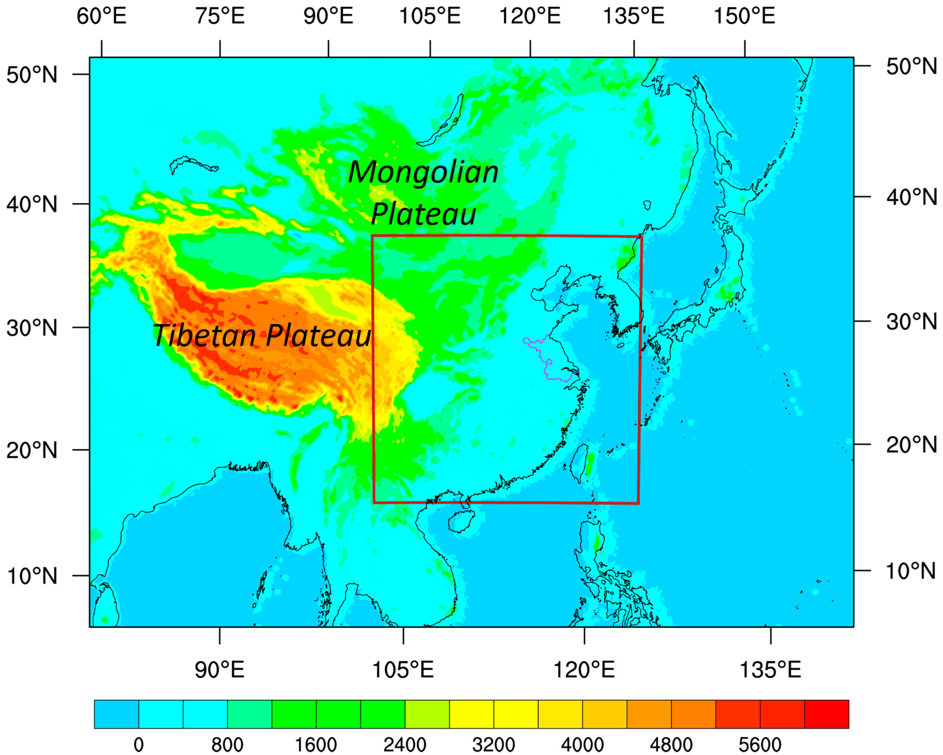
Figure 1. The domains in the PWAFS model and corresponding topography, with the 3 km nested domain marked by the inner brown box. The purple outline denotes Jiangsu Province, China.
Remotesensing 15 03956 g001
Figure 2. Selected transportation meteorological observation stations (marked by the triangles) along the highways (the blue solid lines) in Jiangsu, China. The cities are labeled after the gray lines.
Remotesensing 15 03956 g002
Figure 3. Variations in the MAE ((a) units: °C) and PCC (b) of pavement temperature forecasts at lead times of 3–36 h derived from the LRT and SRMOS models averaged over transportation meteorological observation stations along the Jiangsu highways.
Remotesensing 15 03956 g003
Figure 4. Distributions of the MAE (units: °C) of pavement temperature forecasts at lead times of 6 h (the first column), 18 h (the second column), and 30 h (the third column) derived from the LRT (ac) and SRMOS (df) models along the highways in Jiangsu.
Remotesensing 15 03956 g004
Figure 5. Distributions of the MAESS of the SRMOS pavement temperature forecasts to LRT forecasts at lead times of 6 h (a), 18 h (b), and 30 h (c) along the highways in Jiangsu.
Remotesensing 15 03956 g005
Figure 6. Proportions (Y-axis; units: %) of multiple MAE thresholds (X-axis; units: °C) for pavement temperature forecasts over Jiangsu at lead times of 6 h (a), 12 h (b), 18 h (c), 24 h (d), and 30 h (e) derived from the LRT and SRMOS models.
Remotesensing 15 03956 g006
Figure 7. Scatter plots in pavement temperature for observations (X-axis; units: °C) and forecasts (Y-axis; units: °C) of LRT (ae) and SRMOS (fj), respectively, over Jiangsu at lead times of 6 h (the first column), 12 h (the second column), 18 h (the third column), 24 h (the fourth column), and 30 h (the fifth column). The distance of an individual point to the diagonal refers to the deviation of the forecast from observation. The shading represents the kernel density estimation of the forecast biases. The greater kernel density estimation of a specific point denotes the higher data density of its surroundings, and vice versa.
Remotesensing 15 03956 g007
Figure 8. Boxplot diagrams summarizing the importance distributions (X-axis) of the 10 most important predictors (Y-axis) in the SRMOS model for lead times of 6 h (a), 12 h (b), 18 h (c), 24 h (d), 30 h (e), and 36 h (f). The yellow line across each box and the left and right boundaries of the box refer to the median, lower, and upper quartiles of the importance metrics, respectively. The predictor names can be found in Table 2. The predictors on the Y-axis are sorted in descending order of mean factor importance from top to bottom.
Remotesensing 15 03956 g008
Figure 9. Importance metric distributions of the typical predictors (t2m, q, and gh100) in the SRMOS model for lead times of 6 h (the first column), 18 h (the second column), and 30 h (the third column), respectively.
Remotesensing 15 03956 g009
Table 1. The physical parameterization schemes used in the PWAFS model.
PhysicsScheme
MicrophysicsWRF Single-Moment 6-class scheme [41]
Surface layerMonin-Obukhov [42]
Land surfaceNoah Land Surface Model [43]
Planetary boundary layerYonsei University scheme [44]
Longwave radiationRapid Radiative Transfer Model [45]
Shortwave radiationDudhia scheme [46]
Cumulus parameterizationKain-Fritsch scheme [47,48]
Table 2. Several of the most important predictors in the model and the corresponding abbreviations. p denotes the multiple isobaric levels of 1000 hPa, 950 hPa, 925 hPa, 850 hPa, 700 hPa, 500 hPa, and down to 100 hPa.
Predictor VariablesAbbreviation
Temperature at 2 mt2m
Specific humidityq2m
Dew point temperature at 2 mdpt2m
Relative humidity at 2 mrh2m
Temperature at p hPatp
Geopotential height at p hPaghp
Relative humidity at p hParhp
Dew point temperature at p hPadptp
Disclaimer/Publisher’s Note: The statements, opinions and data contained in all publications are solely those of the individual author(s) and contributor(s) and not of MDPI and/or the editor(s). MDPI and/or the editor(s) disclaim responsibility for any injury to people or property resulting from any ideas, methods, instructions or products referred to in the content.