Cloud Shadow Detection via Ray Casting with Probability Analysis Refinement Using Sentinel-2 Satellite Data

Abstract

Analysis of aerial images provided by satellites enables continuous monitoring and is a central component of many applications, including precision farming. Nonetheless, this analysis is often impeded by the presence of clouds and cloud shadows, which obscure the underlying region of interest and introduce incorrect values that bias analysis. In this paper, we outline a method for cloud shadow detection, and demonstrate our method using Canadian farmland data obtained from the Sentinel-2 satellite. Our approach builds on other object-based cloud and cloud shadow detection methods that generate preliminary shadow candidate masks which are refined by matching clouds to their respective shadows. We improve on these components by using ray-casting and inverse texture mapping methods to quickly identify cloud shadows, allowing for the immediate removal of false positives during image processing. Leveraging our ray-casting-based approach, we further improve our results by implementing a probability analysis based on the cloud probability layer provided by the Sentinel-2 satellite to account for missed shadow pixels. An evaluation of our method using the average producer (82.82%) and user accuracy (75.55%) both show a marked improvement over the performance of other object-based methods. Methodologically, our work demonstrates how incorporating probability analysis as a post-processing step can improve the generation of shadow masks.

1. Introduction

Geographic Information Systems (GISs) are more prevalent today than ever before. The rapid adoption of GIS has been fueled by the increase in the number of satellites orbiting the Earth, which are estimated to be over 4500 [1]. These satellites are important for many purposes, such as communications, navigation, planetary observations, military, radio, and remote sensing. In this work, we focus on remote sensing, the scanning of the Earth by satellite or high-flying aircraft to obtain information, due to being increasingly relied upon in various industries. Remote sensing has many applications such as monitoring ocean temperature, forest fires, weather patterns, growth of urban areas, and vegetation conditions [2]. Due to climate change, monitoring vegetation conditions has become extremely important to ensure the health of forests, wetlands, grasslands, and agricultural sites. Leveraging the data obtained by remote sensing equipment allows us to identify trends and intervene to maximize the health of these ecosystems.

The agriculture industry is a vital aspect of economies and societies around the world. For example, agriculture had a total gross domestic product contribution to the Canadian economy of over 30 billion CAD in 2020 [3]. Smart agriculture employs remote sensing technologies for optimal setting of growing environments to maximize yield (i.e., precision farming). It is unsurprising that remote sensing satellites have become a widely used tool for farming by “increase[ing] production, reducing costs, and providing an effective means of managing land resources” [4] through the means of automated analysis of aggregated farmland satellite data. With this, farmers and farming companies can generate various metrics to estimate crop yield and guide interventions to increase crop production. However, satellite imagery are often fully or partially obscured by clouds and their respective shadows, limiting the effectiveness of such analysis. Directly using data from these obscured regions can produce invalid results. One way to mitigate this issue is to reject images with non-negligible cloud cover. However, if we are able to identify clouds and their shadows within the image data, then partial data could be salvaged and incorporated into analysis. Moreover, the identified shadow regions could be digitally corrected for further use after identification [5,6].

Occlusion by clouds and their shadows impedes any analysis of the underlying regions of interest, and thus, methods identifying clouds and their shadows can improve remote sensing analysis for many other applications (e.g., dark mining locations [7]). Recently, this has led to satellites that provide data that greatly simplify the process of cloud identification. For instance, the Sentinel-2 satellite launched in 2015 takes images of the Earth at a high temporal and spatial resolution (at most 5 day intervals, with a 10 m${}^2$ pixel size for most regions). It also produces several bands that identify cloud-obscured pixels, allowing for their straightforward removal, while bands that can similarly facilitate cloud shadow removal have been investigated, they produce inaccurate results due to the exclusion of cloud shadows from the shadow mask (false negatives) and the inclusion of other structures in the images such as bodies of water or dirt (false positives). See Appendix B, Figure A2c for several example clouds (red) missing cloud shadows (purple) in the scene classification layer (SCL) provided by the Sentinel-2.

There exist many image-based techniques for identifying and removing cloud shadows from satellite images [8,9,10]. However, object-based methods (i.e., constructing a 3D space consisting of the Sun, satellite, clouds, and Earth) are a promising alternative [7,11,12,13]. Object-based methods can infer the position of cloud shadows based on the positions of the clouds in the image. More specifically, if the position of the Sun and the height/geometry of the cloud are known, we can trace the light rays from the Sun through the cloud to determine where the cloud’s shadows are located. This ray-tracing process has been extensively developed for lighting and shading in the rendering of 3D graphics [14]. The results from this technique are impressive, and the base principle for ray casting and ray tracing is utilized in all popular rendering tools, such as Blender and Autodesk 3ds Max, by both amateur and professional rendering production.

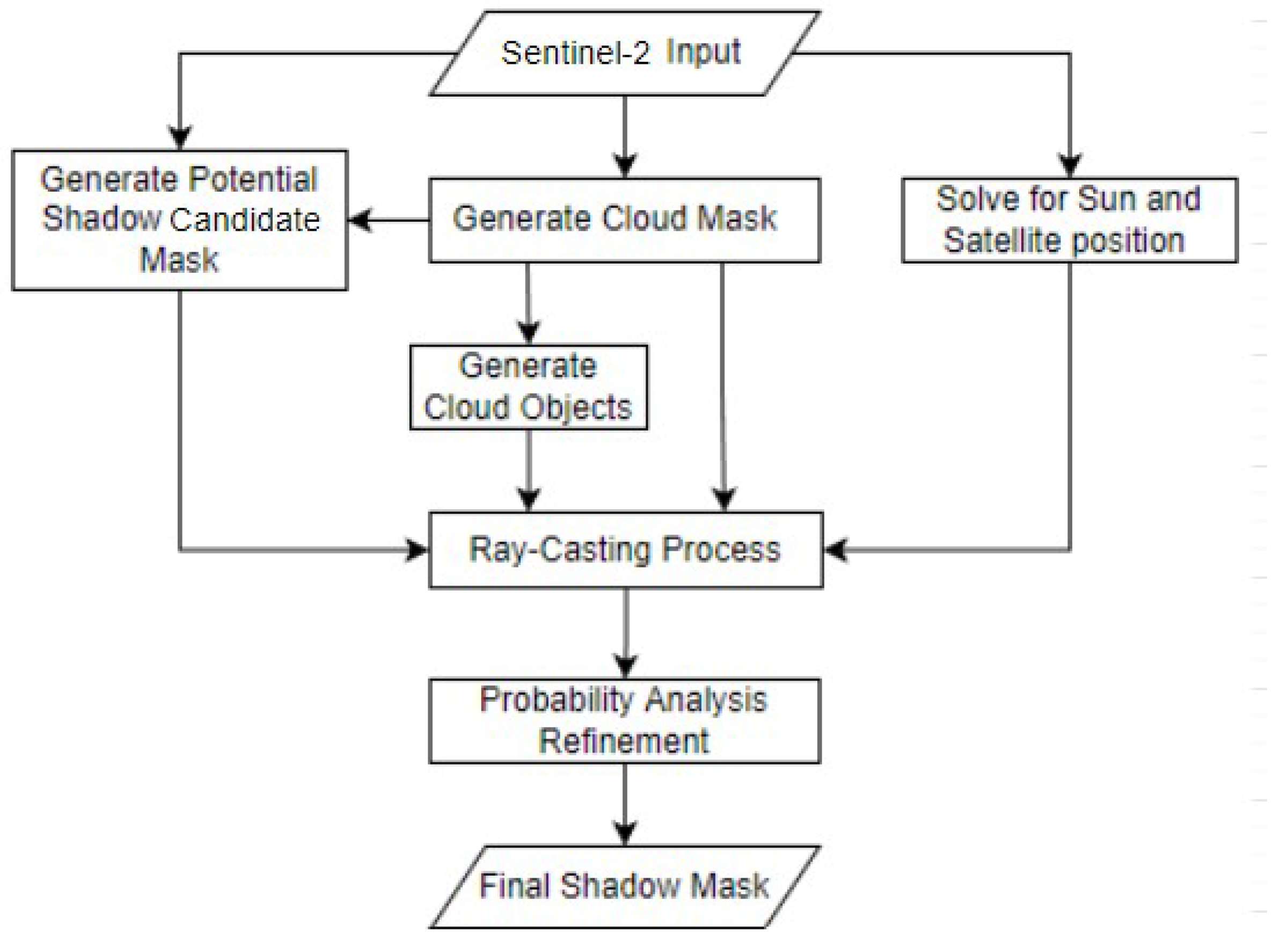
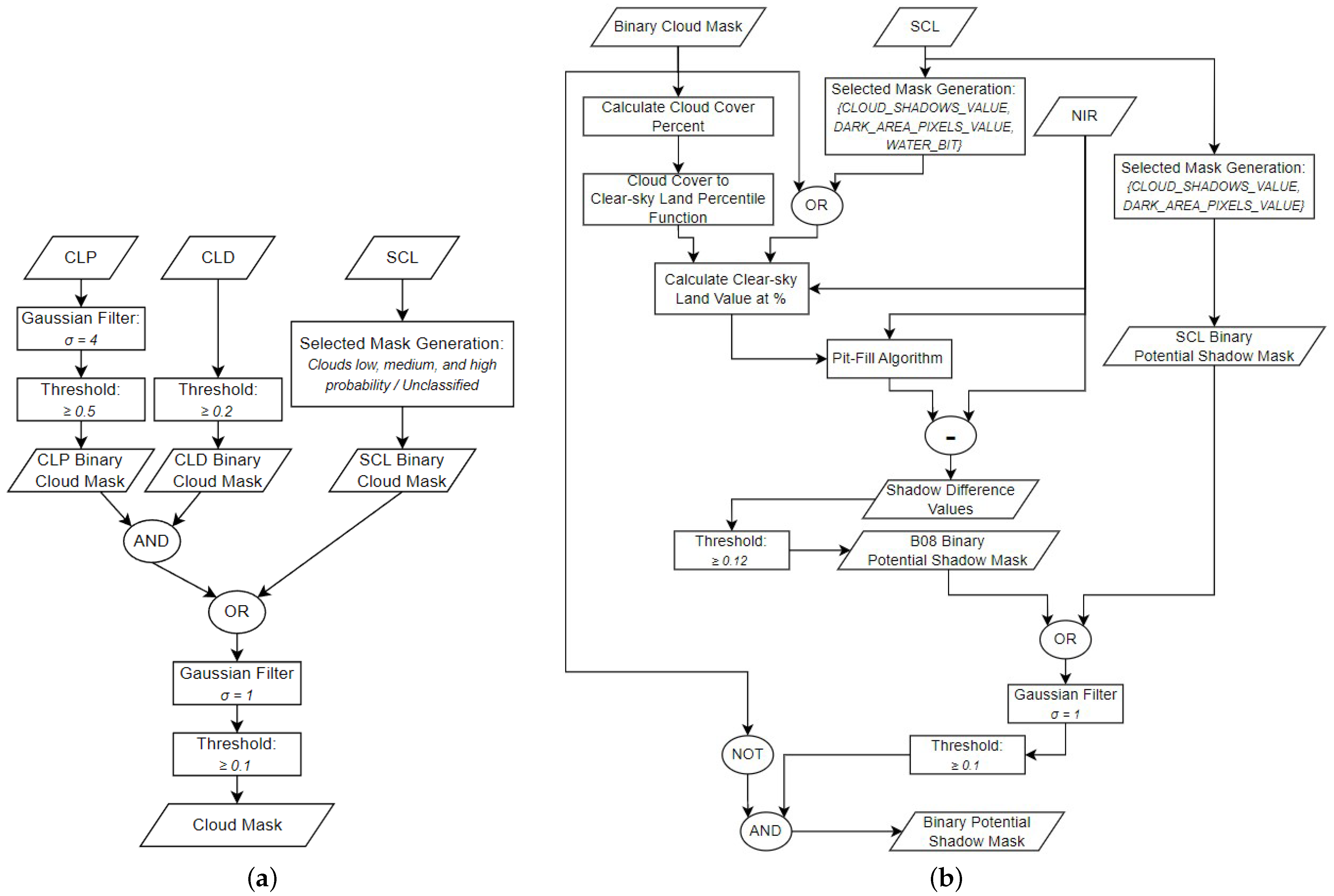
Our method uses ray-casting and probabilistic techniques to improve upon the methods introduced by Zhu and Woodcock [11] and depends on Sentinel-2 GIS imaging. Since Sentinel-2 provides several cloud identification processes, Sen2Cor [15] and s2cloudless [16], we leverage these to generate the cloud mask. The generation of potential cloud shadows builds on the image-based approach described by Zhu and Woodcock [11]. We then use a least squares approach to solve for the optimal global position of the Sun and satellite, relative to the image, utilizing the Sentinel-2 satellite and Sun angle bands. 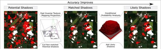Our approach uses a modified version of the object-based method outlined by Zhu and Woodcock [11] for producing a shadow mask by considering various candidate cloud heights for each cloud. Then, using the cloud height and shape and the view/Sun positions, we can produce a shadow mask via efficient ray-casting methods and then shape match these projected shadows against the image-based shadow masks produced in previous steps to find the best match. Finally, we use a novel probabilistic approach to determine the likelihood that each candidate shadow pixel was generated from a cloud shadow and form a final cloud mask by thresholding the probability surface.

To evaluate our method, we selected six datasets from a chosen study area consisting of diverse features (agriculture, villages, bodies of water, barren land, etc.). For each dataset, we manually generated ground-truth shadow masks and compared these masks to those created by successive stages of our method. To compare, we measured the false positive, false negative, and total pixel error percentage normalized to both the number of pixels and the number of shadow pixels in the image. Our analysis showed a clear improvement in the total error percentage for shadow pixels identified in each successive step of the algorithm. The error metrics clearly showed an improvement when adding the novel statistical approach when compared to the ray-casting process output alone. In addition, we used the cloud shadow metrics employed in Zhu and Woodcock’s 2012 paper, the producer and user accuracy [11]. Our method has an average producer accuracy of 82.82% and user accuracy of 75.55%, which is an improvement over the results reported by Zhu and Woodcock [11] (greater than 70% and approximately 50%, respectively). Since our algorithm uses ideas and concepts from computer graphics, an implementation of our algorithm is able to utilize well-established parallelization methods for a computational speedup using commonly available commercial hardware.

Related Work

Due to their importance to problems arising in remote sensing, methods for cloud shadow identification have been extensively studied [17]. We can categorize these techniques into four main types: image processing, temporal analysis, machine learning classification, and geometric relation analysis. It should be noted that many of the processes implemented for cloud shadow detection use more than one of the types listed. Image processing techniques utilize various electromagnetic field (EMF) wavelengths to deduce which pixels are cloud shadows. For example, the US Naval Research Laboratory conducted a study utilizing only the red, green, and blue (RGB) channels of satellites to detect clouds and cloud shadows over ocean water [8]. Next, temporal analysis techniques are closely linked to image processing techniques, but a set of images taken over time are used to compare changes between successive images to determine which pixels are likely cloud or cloud shadows. For example, Jin et al. proposed a method for identifying cloud and cloud shadows by utilizing two-date analysis in Landsat imagery [9]. A limitation of temporal analysis approaches is they require a sufficiently dense temporal sampling data and, thus, if data is sparse, the quality of the result degrades. The next approach is machine learning classification. Leveraging the power of neural networks, algorithms have been produced to identify cloud and cloud shadow data by training a network on previous remote sensing imagery [10]. A recent paper details a method to detect cloud and cloud shadows over mining areas to minimize the misidentification of cloud shadows as mining locations, or vice versa [7]. This approach utilizes a “supervised support-vector-machine classification to identify clouds, cloud shadows, and clear pixels” in the initial identification step [7]. Using the classification results, the last technique of geometric relation analysis, is used to refine the identification data [7]. More specifically, the algorithm projects the centroid of clouds to identify which cloud shadows identified previously are true or false positives. Machine learning can result in very accurate results; however, the system must be trained with a large dataset, requiring substantial temporal data, and is often difficult to fine-tune due to the weak interpretability of machine learning systems [18]. In addition to this, training requires ground-truth data, which is currently being generated manually for our evaluation of our method and is a time-intensive task. This limitation makes it difficult to identify potential improvements, as opposed to geometric analysis methods, where improving the representation of clouds and the rendering of their shadows offer a clear path for improvement.

Zhu and Woodcock propose a series of methods that utilizes image processing and geometric relation analysis [11,12,13]. Their initial method identified candidate clouds and candidate cloud shadows via image processing techniques, then employed a cloud shadow projection technique to eliminate false positive shadows [11].

Our method is similar but distinct from their method. We use a different process to identify clouds, as they use various visual data metrics, such as normalized difference vegetation index, normalized difference snow index, whiteness tests, water tests, and temperature metrics, while our method leverages various cloud data/probability bands provided by Sentinel-2, which is not available in the Landsat satellites, bypassing the issue of Sentinel-2 not having temperature bands. Likewise, the geometric relation analysis of the clouds to their shadows are different. Their algorithm “treats each cloud as a 3D object with a base height retrieved by matching clouds and cloud shadows, and a top height estimated by a constant lapse rate and its corresponding base height” [11] while our method treats each cloud as a 2D object and leverages inverse texture mapping for matching cloud and cloud shadows. This allows our algorithm to project cloud shadows in an effective and efficient manner by only projecting the four corners of a quadrilateral containing the cloud. Our algorithm introduces an additional innovation by adding the probability analysis of the geometric relation analysis output to improve the shadow mask result. Their algorithm has a cloud shadow accuracy of >70% and  50% for producer’s accuracy, related to false negatives, and user accuracy, related to false positives, respectively, (see Section 3 for the definitions of these metrics). Various refinements in their initial method were outlined in subsequent papers, including adding a multi-temporal solution for land cover, a prototype algorithm for the Sentinel-2 satellite [13]. However, the prototype algorithm for the Sentinel-2 satellite was not used directly for our algorithm, though similarities exist since their method is also based on their original method proposed for Landsats 4–7. Both methods treat the cloud as a flat planar object and both utilize cloud probability metrics to generate the cloud mask. Our algorithm surpasses the prototype algorithm by implementing the novel probabilistic method to further refine the results after the ray-casting method.

2. Materials and Methods

2.1. Study Area, Conditions, and Data Sources

The chosen area of study is farmland located in the WGS84 region $(51.256758,$$-113.639145)$ to $(51.449300,-113.329468)$, and was chosen due to the various types of terrain features it contains, as highlighted in Figure 1. By using this plot of land for every test, we can directly compare the results between different cloud cover conditions and control errors introduced by variation in the underlying terrain. Using this area of study, six datasets were chosen during the summer of 2020, as listed in

Table 1. The six chosen dates to be analyzed reside in the same 22.3 km by 20.7 km patch of land located in the region $(51.256758,-113.639145)$ to $(51.449300,-113.329468)$, as seen in Figure 1. Each date reports the percentage of cloud cover, whether thin stratus or “wispy clouds” are present and whether cirrus clouds were detected by the s2cloudless process.

Date	Cloud Cover %	Thin Stratus or “Wispy” Clouds	Cirrus Clouds
15 June 2020	6%	No	No
25 June 2020	1%	No	Yes, light haze over the image
27 June 2020	20%	Yes	Yes
5 July 2020	10%	No	No
20 July 2020	7%	No	No
22 July 2020	15%	No	No

.

As the application for this paper is farmland satellite image analysis during the growth season, the months used for the study range from May to August, with a focus on June and July, where maximum crop growth is likely to occur. As such, images with snow and ice were not considered. However, to facilitate discussion around the effectiveness outside the intended seasons, additional datasets were used as examples in Section 4. Furthermore, with farmland being the focus, any bodies of water in the scene are assumed to be small relative to the study area size. Lastly, since the application is designed to use partial images for additional data, cases where there were negligible usable data due to almost total cloud cover were discarded.

Since the resulting cloud shadow mask is used to obscure corrupted data, incorrectly identifying valid pixels as clouds (false positives) are preferred to false negative cloud shadows, as it is better to omit correct data compared to including incorrect data as this will bias the analysis, potentially invalidating the results.

All data used for the algorithm are sourced from the Sentinel-2 satellite, located on Sentinel Hub’s servers [19]. The bands used were the near-infrared (NIR) band, the scene classification layer (SCL), the cloud probability layers (CLP and CLD), and the four angle layers (two azimuth and two zenith layers) to determine the direction of the Sun and satellite relative to the pixel. For clarity, we will be referring to the cloud probability layers CLP and CLD as CLP₁ and CLP₂, respectively. More information on the bands can be found in Sentinel Hub’s documentation [19].

2.2. Methodology

Our approach first generates a broad set of potential cloud shadows, stored in a shadow mask, and then geometrically prunes the set of false positive shadows until only the correct cloud shadows remain in the mask, after which we apply post-processing methods to further refine the result. Our method can be broken down into several steps, as detailed in Figure 2. First, we generate our cloud mask and partition it into individual cloud objects (Section 2.2.1). Second, we generate our potential shadow candidate mask, which identifies which pixels are likely to be clouds (Section 2.2.2). Third, we form a 3D scene by solving for the global positions of the satellite and Sun with respect to the images (Section 2.2.3). Fourth, each cloud is tested to find its respective shadow, if visible, by using ray-cast projection onto the Earth’s surface for shape matching between projected shadows and shadows in the candidate mask (Section 2.2.4). The final step is to generate a statistical model that improves the final generated cloud shadow mask (Section 2.2.5).

2.2.1. Cloud Detection

To utilize the geometric relation between clouds and cloud shadows, the clouds in the scene must be first identified and partitioned into separate cloud objects. Sentinel-2 has two processes to detect clouds. One process is the s2cloudless system [16] that generates two bands: the cloud probability (CLP₁), which is a grayscale image with larger values indicating a higher probability of a cloud being present, and the cloud mask (CLM), which is a binary mask indicating if the pixel in question should be considered to be obscured by a cloud [20]. These bands have a resolution of 160 m and are far too coarse to be directly utilized for high-precision analysis, particularly the CLM. Furthermore, the CLM generated by the s2cloudless system [16] can have a high degree of error due to the exclusion of small clouds or severely overestimate the size of clouds and, thus, is not used. The second process for detecting clouds in the Sentinel-2 system utilizes the Sen2Cor processor [15]. The Sen2Cor processor [15] generates two relevant bands: the scene classification mask (SCL), which categorizes the pixels into various categories including clouds, and the cloud probability (CLP₂), which is different from the CLP₁ mask discussed before. These bands have a resolution of 20 m, which is much better than the resolution of 160 m; however, these bands tend to underestimate the amount of cloud in the scene, particularly for semi-transparent clouds. As such, we developed an alternate method specifically for Sentinel-2 utilizing both processes’ outputs to generate the cloud mask.

Our method uses the CLP₁, CLP₂, and SCL bands generated by Sentinel-2, which we further process and combine to generate the cloud mask, as seen in Figure 3a. The idea is to generate a cloud mask from the two probabilities where they agree. More specifically, if both are above a certain threshold, then the likelihood of a cloud in the region is high, thereby producing a higher confidence cloud mask. Since the CLP₁ has a 160 m resolution, it is first passed through a Gaussian filter. Next, the CLP₂ and smoothed CLP₁ are passed through a threshold filter to produce two binary cloud masks and subsequently combined by taking the conjunction between the results. This combined result indicates where the two processes agree; thus, the confidence of the mask is increased. Since the SCL mask appears to be more conservative with respect to cloud detection and, thus, more reliable when they are indicated as clouds, the cloud pixels in the SCL mask are added to the previous result. To finalize the cloud mask, the previous result is passed through a Gaussian filter and threshold filter to smooth any harsh edges resulting from combining the three bands, producing the final cloud mask.

Since the clouds captured in the scene are likely to be at varying altitudes, each cloud is projected and tested separately to identify its shadow. Individual clouds are defined by separating cloud pixels into connected components. We apply a flood-fill algorithm [21] using the eight neighbors of each valid cloud pixel to identify all the clouds in an image. Any cloud that is extremely small (only a few pixels) is removed from the individual cloud list used to identify cloud shadows, as clouds of these sizes are typically errors or are too small to generate visible shadows at the resolution captured by satellites.

2.2.2. Candidate Shadows

Sentinel-2 does not provide ready-to-use data on cloud shadows as it does for clouds, while there is a pixel value reserved for cloud shadows in the SCL mask, most shadows in the scene are missing or poorly identified, as seen in Appendix B, Figure A2c. As noted by Zhu and Woodcock, the near-infrared band (NIR) is related to cloud shadows via longer wavelengths in cloud shadow regions [11]. Therefore, areas with low NIR intensities with a high contrast compared to their surroundings are more likely to be cloud shadows. Treating the NIR band as a height map, local minima or pits relative to their surroundings correspond to potential cloud shadows [11]. Following this intuition, Zhu and Woodcock [11] leveraged the morphological pit-filling algorithm [22], also known as the morphological flood-fill transformation, to deduce the relative pit depths to identify potential shadows by comparing the pit-filled result to the original. Our method uses a modified version of this approach.

Our modified method utilizes the NIR band, the cloud mask generated previously, and the SCL mask (see Figure 3b). To perform the pit-filling algorithm, a boundary value surrounding the NIR band must be defined to propagate the morphological drainage simulated by the algorithm. When pits intersect with the boundary of the NIR-band image, the boundary value replaces the edge of the cloud that was cutoff by the image boundaries. Therefore, the fill level for boundary intersecting pits is heavily influenced by the boundary value chosen, as this essentially defines the depth of these pits. This value should represent standard NIR values not obscured by cloud shadows in any given NIR band. The effect the boundary value has on the resulting pit-fill can be seen in Figure 4, in the first row. Due to the variation in the unobscured (by cloud or shadow) NIR values between datasets, the boundary value must be determined per dataset. A fixed boundary value will either miss smaller impact cloud shadows near the border or many false positive shadows will be included and reduce the accuracy of the subsequent shape-matching procedure, depending on if the fixed value is too low or too high, respectively. This can be seen in Figure 4. By assuming most of the unclouded portions are not covered in water, we can compile a list of NIR values from pixels in the image not obscured by a cloud in the derived cloud mask or labeled as cloud shadows, dark areas, or water in the SCL mask and take a value as a percentile directly. As we do not know which pixels are cloud shadows, we obtain an appropriate clear-sky NIR value by leveraging the fact that the clear-sky NIR percentile depends on the amount of cloud shadow, which, in turn, is roughly proportional to the amount of clouds. Using the cloud cover percentage from the generated cloud mask, we apply a sigmoid function to these values to obtain a smooth transition from cloud cover to clear-sky NIR percentile. Consequently, as cloud cover increases, the clear-sky NIR percentile likewise increases to compensate for the increase in cloud shadows present. Unlike Zhu and Woodcock [12], our algorithm does not require or utilize temperature information (as Sentinel-2 does not provide this information). As such, this method for determining cloud shadows would work for other satellites that do not include temperature data.

Using the calculated boundary value, the pit-filling algorithm [22] can be performed, and the difference between the filled and original NIR band is passed through a threshold filter to produce an intermediate result. In Figure 4, the effect of the boundary value on the pit-filled, difference, and threshold result can be seen. With the intermediate result and a shadow mask generated from pixels labeled as shadow and dark areas in the SCL, we perform a disjunction between the intermediate result and the generated shadow mask and pass it through a Gaussian filter and threshold filter to smooth the result. Lastly, to clean up the result, any pixel labeled as a potential shadow in the smoothed result and a cloud in the cloud mask is cleared of its shadow status to generate the candidate mask. An example candidate mask result, along with the cloud mask generated before, can be seen in Figure 5. As seen in Figure 5, there are many potential shadows identified, many of which are not cloud shadows, such as lakes and dark areas. These false positives are removed in later steps.

2.2.3. Satellite View Point and Sun Position

In order to correctly project shadows from clouds onto the candidate mask, we first need to find the view (satellite) position and Sun position relative to the image data. These points define two perspective projections of the cloud, relative to the satellite and Sun, respectively, and are vital to correctly identify the correlation of clouds with their respective shadows (Section Ray-Casting Scene). Sentinel-2 provides four angle bands to determine these relative locations: the Sun zenith angle, the Sun azimuth angle, the view zenith angle mean, and the view azimuth angle mean. For each pixel, two direction vectors can be calculated, one for each projection. Using the pixel locations as the origin of the vectors, two grids of direction vectors, each pointing to the Sun and satellite, can be generated. However, as depicted in Figure 6, due to the 5000 m resolution of the angle bands, the resulting direction grids do not converge at a single point and, thus, do not represent a global perspective projection. Surveying the existing literature, this problem does not appear to have been addressed in previous works. As such, we introduce a method to approximate the Sun and satellite as global points determined by using the least squares method. More specifically, the global point X minimizes the squared distance to all the lines defined by the direction vector and position pairs. Through experimentation with the data, it was found that the direction vectors generated were too coarse to consistently generate a reasonable height for our optimal position. Consequently, a height constraint was added to restrict the height (z component of X) based on measured values of 150,000,000 km for the Sun and 785 km for the satellite. We used the Lagrange multiplier method to form the corresponding constrained least squares problem [23] (Equation (1)), from which we derived, and the linear system of equations that is solved to obtain X (Equation (2)).

Proceeding more formally, we will use the notation “$\widehat{·}$” to denote a unit vector, “$\overrightarrow{·}$” to denote a vector, capitalized non-bold letters to denote points, and capitalized bold letters to denote matrices. Given a set of 3D direction vector and position pairs, each denoted as $({\widehat{d}}_i,P_i)$, on the plane, $z=0$, and the specified height constraint of value, h, we need to solve the minimization problem:

$$\begin{array}{c}\hfill \begin{array}{c}\hfill f\left(X\right)=\underset{X}{min}\sum _i{\parallel (X-P_i)-\left({(X-P_i)}^T{\widehat{d}}_i\right){\widehat{d}}_i\parallel }^2,\end{array}\\ \hfill \mathrm{subject} \mathrm{to}\begin{array}{c}\hfill g\left(X\right)=X^T\left[\begin{array}{c}0\\ 0\\ 1\end{array}\right]-h=0.\end{array}\end{array}$$

(1)

Equivalently, we solve ${\nabla }_{X}f\left(X\right)-\lambda {\nabla }_{X}g\left(X\right)=0$, subject to the preceding height constraint. This yields the following augmented linear system of equations: $\mathbf{A}{X}^{*}=\overrightarrow{b}$, where

$$X^{*}=\left[\begin{array}{c}X\\ \lambda \end{array}\right], \mathbf{A}=\left[\begin{array}{cc}2{\displaystyle \sum _i}[\mathbf{I}-{\widehat{d}}_i{\widehat{d}}_i^T]& \begin{array}{c}0\\ 0\\ 1\end{array}\\ \begin{array}{ccc}0& 0& 1\end{array}& 0\end{array}\right], \overrightarrow{b}=\left[\begin{array}{c}2{\displaystyle \sum _i}[P_i-\left(P_i{\widehat{d}}_i^T\right){\widehat{d}}_i]\\ h\end{array}\right].$$

(2)

To verify that the Sun and satellite position were correctly determined, we tested the results from the six datasets from Table 1. For each scene, the mean dot product between the direction vector at each pixel and the direction pointing from each pixel to the calculated positions was calculated. The results of this analysis can be seen in

Table 2. Results determining the accuracy of the Sun and satellite position in the six datasets described in Table 1 using the mean dot product.

Date	Sun	Satellite
15 June 2020	0.99999994	0.99999785
25 June 2020	0.99999994	0.99999809
27 June 2020	0.99999994	0.99999231
5 July 2020	0.99999994	0.99999851
20 July 2020	0.99999994	0.99999791
22 July 2020	0.99999994	0.99999321
Average	0.99999994	0.99999631
Angle 1	0.02${}^{\circ }$	0.16${}^{\circ }$

¹ Obtained using the inverse cosine function.

, and it showed the Sun’s mean dot product was 0.99999994 and the satellite’s mean dot product was at least 0.99999 in all tested cases. Through testing, it was found that increasing the height of the satellite had a negligible effect on the mean dot product. However, decreasing the height of the satellite had a non-negligible effect on the mean dot product only when decreased below 100 km. Above 100 km, the mean is within 0.1% of 1. As such, the alternate method of orthogonal projection used in other methods [7] could be used instead.

2.2.4. Ray-Casting Scene

Geometrically, determining the location of a cloud’s shadow requires knowledge of the cloud’s height from the surface. However, this information is lost when the satellite’s bands are projected on the satellite’s camera lens. We determine the cloud’s height by iterating over a range of heights and computing the resulting 2D shadow using ray casting [13]. We then use the height that maximizes the similarity between the projected shadow and the candidate mask [13].

Repeatedly ray casting for each cloud pixel to identify the optimal height, h, is computationally expensive. We simplify this computation by representing each cloud as a planar quadrilateral (the 2D bounding box of the cloud), $Q_c$, and assume the surface below is relatively flat. Under these simplifications, for a given h, the projected shadow can be determined by two perspective projections, as seen in Figure 7. The corners of $Q_c$ are projected from the Earth’s surface to the plane situated at h, with the view (satellite) position being the focal point producing the quadrilateral, $Q_i$. Next, the quadrilateral is projected back onto the Earth’s surface using the Sun as the focal point producing the quadrilateral, $Q_s$. Using these projections, we find the transformation mapping $Q_c$ to $Q_s$, $M=P_{i\to s}{P}_{c\to i}$, where $P_{c\to i}$ and $P_{i\to s}$ are the first and second perspective transformations, respectively.

Using $Q_s$, we can iterate through the pixels in the shadow map that are contained within $Q_s$ to compare the similarity between the candidate mask to $Q_s$, the shadow. The projected shadow, $Q_s$, may not be exactly pixel-aligned with the candidate mask. Inverse texture mapping using $M^{-1}$ is applied to transform the pixel coordinates in the candidate mask to pixel coordinates in the cloud mask, the source of the projected shadow. To determine the similarity, a series of tests are applied to each pixel in the shadow mask that are contained within $Q_s$. First, if a pixel in the shadow mask (before applying inverse texture mapping) is labeled as a cloud in the cloud mask, the pixel is ignored since it cannot be both a cloud and a cloud shadow. Next, $M^{-1}$ is applied, and the following tests are performed:

1.

If the transformed pixel indexed into the cloud mask does not belong to the desired cloud, then it is ignored. If so, then increment the total projected shadow pixel count, T, and move to the next test.

2.

If the transformed pixel indexed into the shadow mask is labeled as a potential shadow, then increment the total number of correctly identified shadow pixels, C.

Once complete, the similarity can be determined by the ratio $S=\frac{C}{T}$. The metric S ranges from zero to one, with zero being no similarity and one being perfect similarity. It should be noted that the similarity comparison omits any pixels that fall outside the image boundaries, and as mentioned before, pixels that are labeled as cloud pixels before applying $M^{-1}$ are not included in C or T, thereby removing biases related to shadows being obscured by clouds.

By applying this process, we can apply the iterative method presented by Zhu and Woodcock [13]. That is, we iterate h starting at 200 m, and ending at 12 km. Progressing through the iterations, the result that maximizes the similarity is saved. After completion, if the max similarity found is below the minimum threshold similarity of $0.3$ [11], the result will be discarded, as it is assumed that the cloud shadow is not visible in the image data. This often occurs when the angle between the Sun and the satellite is small, another cloud is obscuring the shadow, or the cloud is thin enough to not produce a detectable shadow. Once the iteration process has been completed for all clouds, the object-based shadow mask (shadow mask resulting from the ray-casting process) is generated by all the pixels that are both in the potential shadow mask and under one or more cloud shadows, resulting in the exclusion of pixels determined to be false positive shadows in the potential shadow mask. Figure 8 is the resulting object-based shadow mask from the results depicted in Figure 5.

2.2.5. Statistical Improvements

While the method in Section 2.2.4 correctly identifies many cloud shadow pixels, it tends to introduce false negatives at the edge of cloud shadows. By leveraging the cloud probability bands provided, we can correlate the cloud probability to the cloud’s shadow to construct a shadow probability for improving the shadow detection accuracy. To do this, we analyze non-cloud shadow pixels and determine if they should be added to the shadow mask based on their probability values. In this technique, we model a conditional probability surface, $P\left(\alpha \right|\beta ):$ the probability that a pixel with a shadow value of $\alpha$ is classified as shadow given that it has a shadow projected probability of $\beta$. This probability surface is constructed and utilized for the entire image, taking the surrounding regions unaffected by clouds or cloud shadows into account.

The shadow value, $\alpha$, is derived from our potential shadow candidate mask generation process. More specifically, using the difference between the pit-filled and original NIR band, we can derive the shadow value, $\alpha$, while the direct difference provides an indicator of the shadow’s probability, the data are heavily biased toward 0, rather than being evenly distributed between 0 and 1, resulting in a poor probability surface quality as most of the data will be concentrated in a subsection of the surface. To correct this, the shadow value used is derived by passing the difference through a normalized sigmoid function (Equation (3)) to redistribute the values more evenly.

$$S\left(\alpha \right)=\frac{f(\alpha -0.5)-f(-0.5)}{f\left(0.5\right)-f(-0.5)}, \mathrm{where} f\left(x\right)=\frac{1}{1+0.007e^{-17x}}.$$

(3)

The shadow projected probability, $\beta$, is derived from the provided cloud probability and the ray-casting process. Using the same optimal M transformation used to project each cloud to their respective shadows (defined in Section 2.2.4), we project the smoothed CLP₁ layer (from Section 2.2.1) for each M to generate the shadow projected probability map. However, simply projecting and writing the probability values to our new probability map using $Q_s$ (only pixels contained in $Q_s$) is not sufficient, as this will introduce edge artifacts. Furthermore, since the cloud mask inherently contains some error, some cloud probability values in the smoothed CLP₁ are not contained in $Q_s$, which are mostly distributed around the edge of the cloud, thereby limiting the improvement in the shadow mask. If we project the entire smoothed CLP₁ layer, however, cloud probability artifacts from other clouds will be projected along with the desired cloud for each M, introducing errors into the shadow projected probability map.

To solve this, we implemented a method where the entire smoothed CLP₁ is projected, but the probabilities are weighted by distance to the projected shadows determined in Section 2.2.4. More formally, a maximum influence distance, D, for each cloud is defined, where every probability outside this distance has a 0 weight. Correctly selecting D allows the surrounding probabilities for a cloud to be considered but will exclude other clouds for the given M. Through experimentation, it was determined that as the area of a cloud, A, increases, D should increase as well to adequately recover missed pixels. After testing a $D\propto A$ relationship, it was determined that the increase in D was too large for larger cloud sizes. As such, a $D\propto \sqrt{A}$ relationship was considered and produced much better results, particularly when we clamped D to an appropriate interval. Any pixel inside the projected shadow from Section 2.2.4 will have a weight of 1. Between the edge of the projected shadow and the distance equals the D boundary, and the weights will be calculated by a quadratic radial basis function that decreases as the distance increases. Note that this function is continuous, so adjacent pixels will have similar weights.

Using the above process, we project the smoothed CLP₁ using every M and write the projected cloud probability (multiplied by the appropriate weight) to our shadow projected probability map. In some cases, projected probabilities will overlap. As such, the value in the map will retain the maximum value. An example output of the shadow projected probability map can be seen in Figure 9.

Now that we have the shadow value and projected shadow probability for every pixel, we construct the conditional probability surface of the form $f(\alpha ,\beta ):[0,1]\times [0,1]\stackrel{}{\to }[0,1]$. For more detail, the following algorithm is outlined in Appendix A. The surface is modeled as a bi-linearly interpolated surface with the height, $f(\alpha ,\beta )$, defining $P\left(\alpha \right|\beta )$ for a given $\alpha$ and $\beta$. Using the object-based shadow mask generated from Section 2.2.4, we assign a binary value indicating if a pixel is in a shadow or not. This value represents a collapsed state of $f(\alpha ,\beta )$ for the pixel sample and will be 0 and 1 for non-shadow and shadow pixels, respectively, (see Figure 10a). We can generate the probability surface by approximating the value of $f(\alpha ,\beta )$ at any given $\alpha$ and $\beta$ value (see Figure 10b). To do this, $\alpha$ and $\beta$ values are partitioned into regular grids with each grid cell storing the average of all the pixels located in the cell boundary. These average values are used to generate a piece-wise linear probability surface. However, if the grid partition is too coarse, many fine details will be missed. On the other hand, if the grid partition is too fine, then the quality of the resulting surface could suffer by the degradation of the cell averages as a result of having little or no samples contained in cells. To address this, we construct multiple surfaces at various levels of partition resolution and aggregate them to produce a single probability surface. Through experimentation, the chosen partition resolutions are $8,16,32,64,$ and 128. Finally, to construct our final surface, we regularly sample (we chose 256 by 256 samples) each surface and take the weighted sum of the results. To preserve the overall shape of the surface while including fine details, the chosen weights are biased towards the coarse surfaces. More specifically, the values are the normalized weights of $\frac{16}{31},\frac{8}{31},\frac{4}{31},\frac{2}{31},$ and $\frac{1}{31}$. To resolve cells on the intermediate surfaces with no pixels contributing to the cell’s average, a $3\times 3$ average kernel is applied over the missing pixels until a value is determined. The final surface is dominated by low-resolution surfaces, which rarely has missing cells, so the approximation of the averages at higher resolutions is sufficient to generate a high-quality probability surface. For a visualization of an example of the resulting probability surface, see Figure 11.

Using this surface, we can test every pixel in the data and use their $\alpha$ and $\beta$ values to obtain the probability of a cloud shadow being present. A minimum threshold is set, 0.15 (Figure 11), and every pixel with a sufficiently high probability according to the minimum threshold will be added to the cloud shadow mask to produce the final shadow mask, as seen in Figure 12.

Considering false negatives and false positives in more detail, the ray-casting algorithm that generates the object-based shadow mask removes many false positives at the expense of increasing the number of false negatives. This is an expected result, as eliminating potential shadow pixels will inevitably remove true shadow pixels in error as well, and may be a consequence of errors in the cloud mask or shape-matching algorithm. Applying the probability analysis, the false negatives are decreased by adding the missed pixels back into the image; however, some false positives are likely to be generated.

3. Results

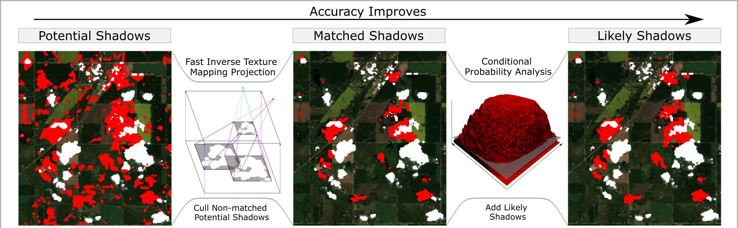
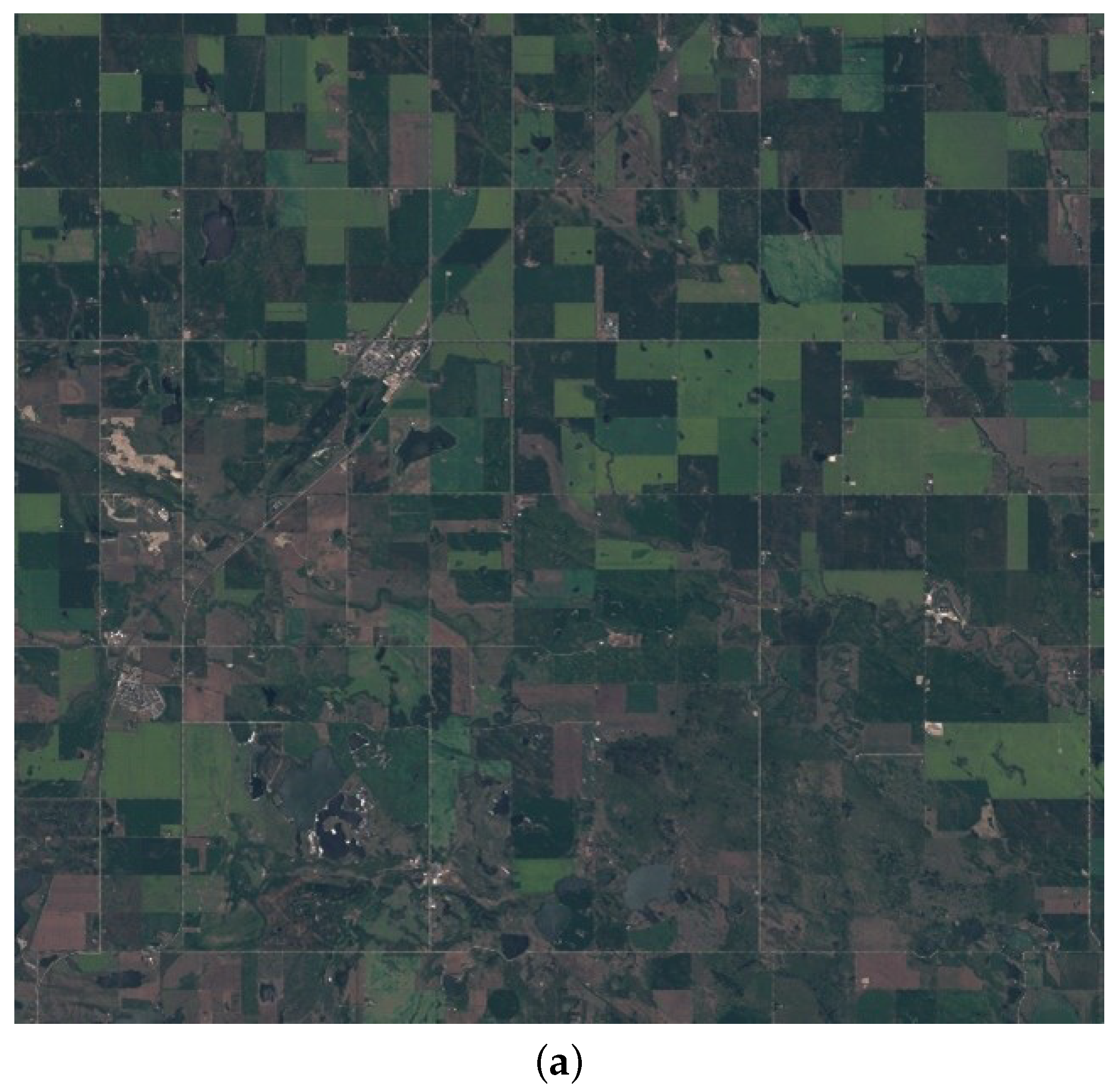
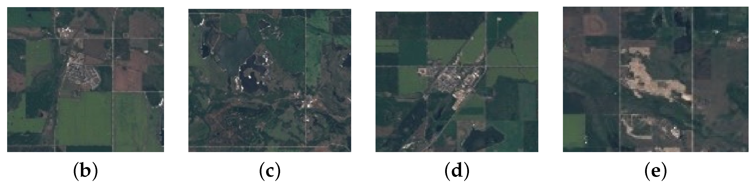
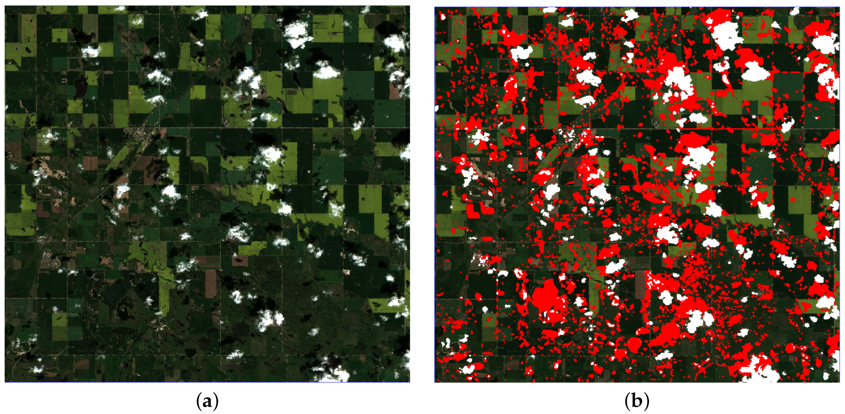
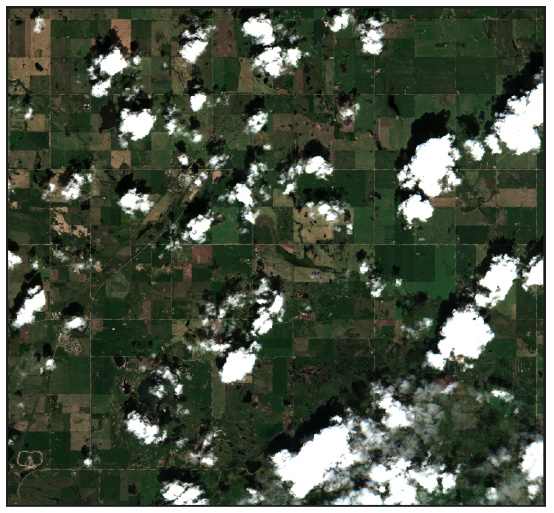
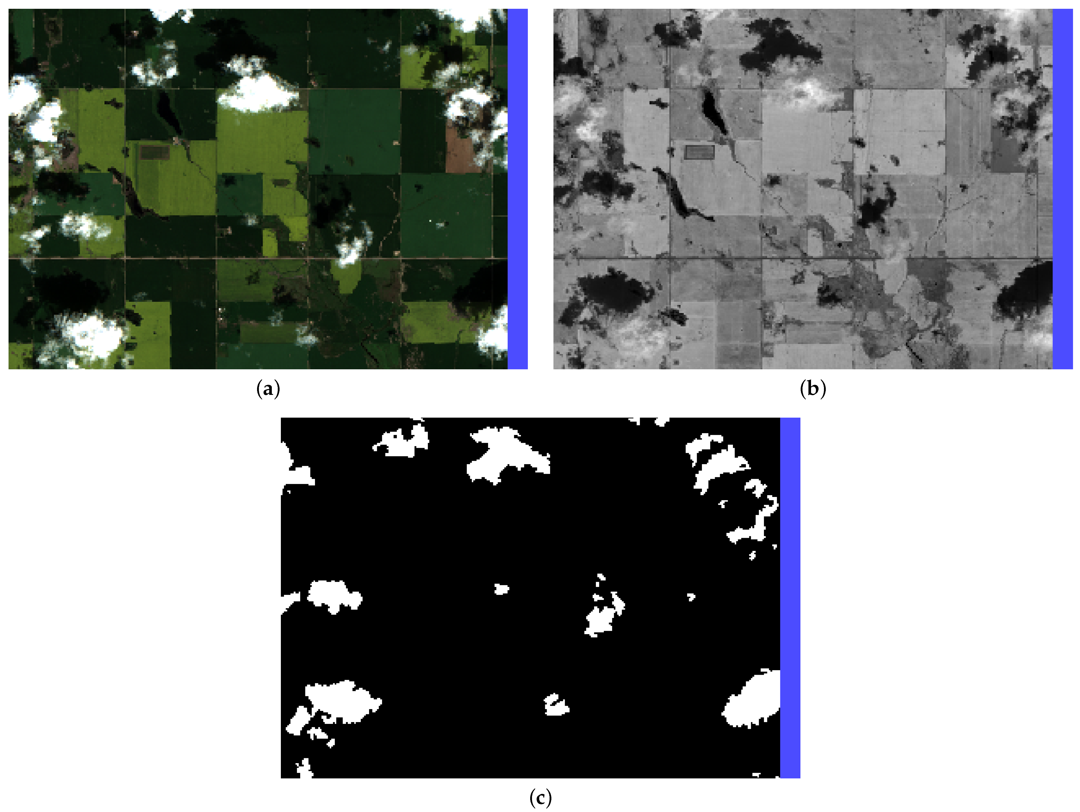
For evaluating our method, we chose a study area with diverse features (Figure 1), ensuring we have variation in the underlying surface in a controlled manner for comparisons between datasets. Using the test datasets described in Table 1, we evaluated the shadow masks generated by our method to determine their suitability. Our method produces three different shadow masks, and in order to understand how well each phase of the method was affected our results, we evaluated the shadow masks produced at each stage, including the candidate shadow mask, object-based shadow mask, and final shadow mask. For each mask, we compared it to a baseline ground-truth image manually generated by the authors. Figure 13b shows one of these manually generated images. When creating the baseline, there is inherent ambiguity regarding the state of each pixel (shadow or not shadow), leading to some human error. This ambiguity was particularly notable around areas where cloud edges intersected underlying shadows, resulting in increased uncertainty. In this situation, pixels that could not be definitively classified as either shadow or cloud were assigned as shadow pixels. We did this without effecting the error metric calculations because either the pixel is truly a shadow pixel or is a cloud pixel and removed from the metric calculations.

Using this ground-truth shadow baseline, we evaluated the predictive accuracy error of the three shadow masks, for each of the six datasets, based on the six metrics in

Table 3. Error metric calculations used to compare various stages of our shadow detection algorithm. False positive pixels are classified as shadow pixels according to the mask, but not in the shadow baseline. Likewise, false negative pixels are classified as shadow pixels in the baseline image, but not according to the mask. False pixels are identified as either false negative or false positive. AllPixels is the number of pixels in the evaluation region and ShadowPixels is the number of pixels that are labeled as shadows in either the shadow mask or shadow baseline in the evaluation region.

Metric Name	Function
False Positive Error Relative to Image Size	$E_{FP,I}={\displaystyle \frac{\sum FalsePositives}{\sum AllPixels}}$
False Negative Error Relative to Image Size	$E_{FN,I}={\displaystyle \frac{\sum FalseNegatives}{\sum AllPixels}}$
False Pixels Relative to Image Size	$E_{F,I}={\displaystyle \frac{\sum FalsePixels}{\sum AllPixels}}$
False Positive Error Relative to Shadow Pixels	$E_{FP,SP}={\displaystyle \frac{\sum FalsePositives}{\sum ShadowPixels}}$
False Negative Error Relative to Shadow Pixels	$E_{FN,SP}={\displaystyle \frac{\sum FalseNegatives}{\sum ShadowPixels}}$
False Pixels Error Relative to Shadow Pixels	$E_{F,SP}={\displaystyle \frac{\sum FalsePixels}{\sum ShadowPixels}}$

. Each metric was normalized to yield a pixel percentage, with $0\%$ indicating that no errors were found and the shadow mask perfectly reproduces the ground-truth shadow baseline. Finally, to facilitate a direct comparison between our results and those reported by Zhu and Woodcock [11], we also report the cloud shadow producer accuracy and cloud shadow user accuracy (Equations (4) and (5)). These metrics represent the predictive accuracy of our masks with regard to missed shadow pixels (false negatives) and the inclusion of non-shadow pixels (false positives). 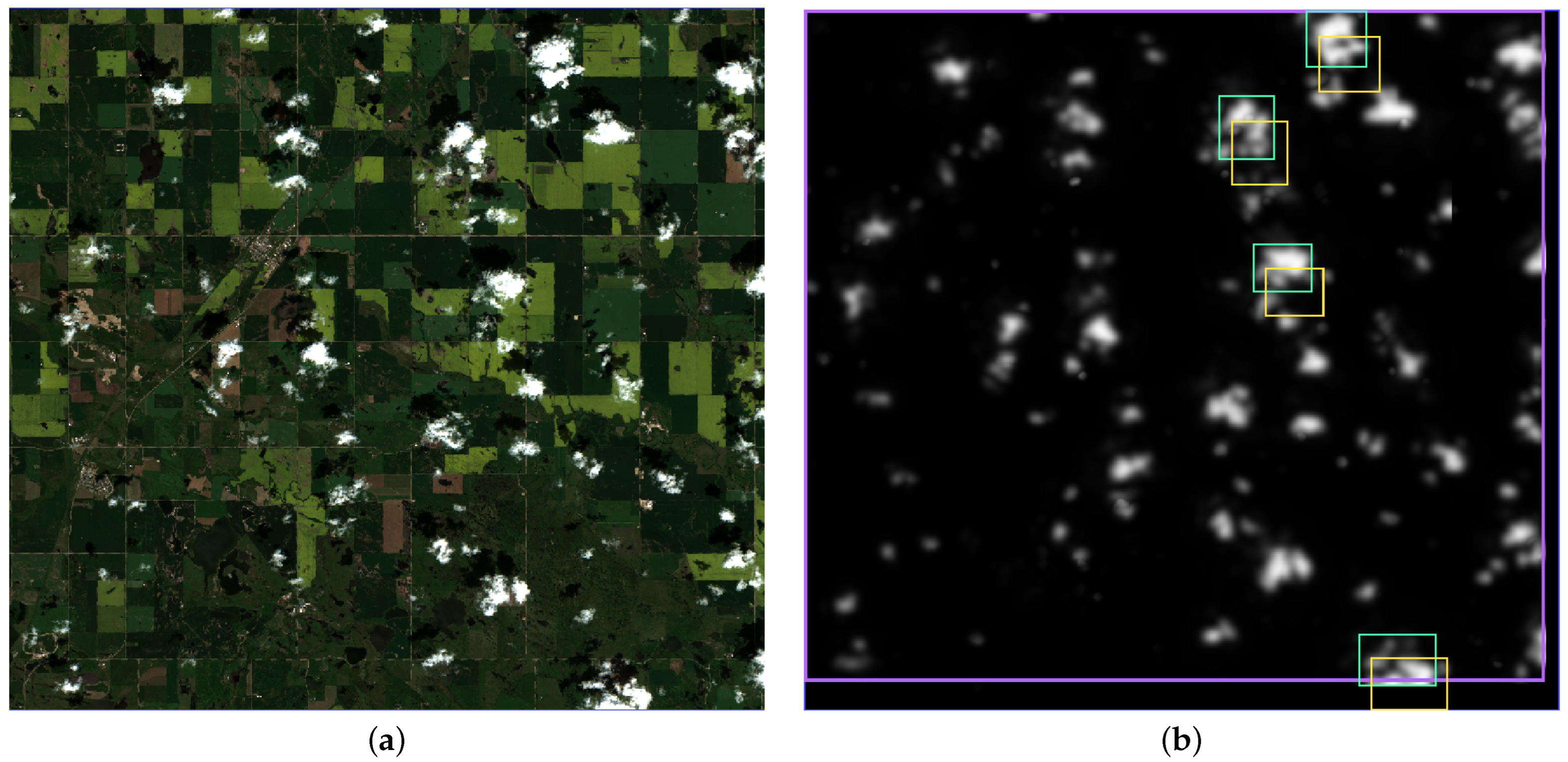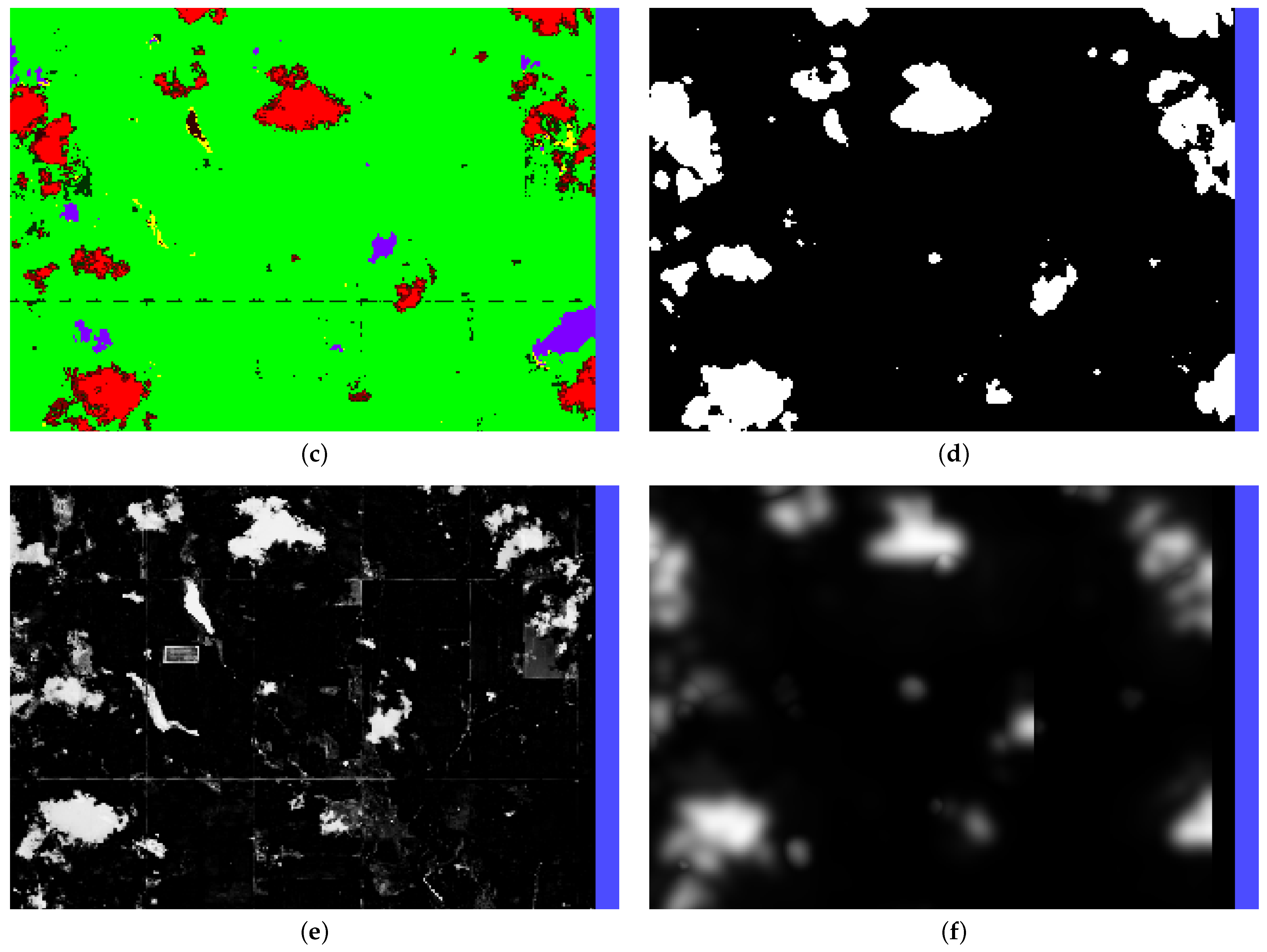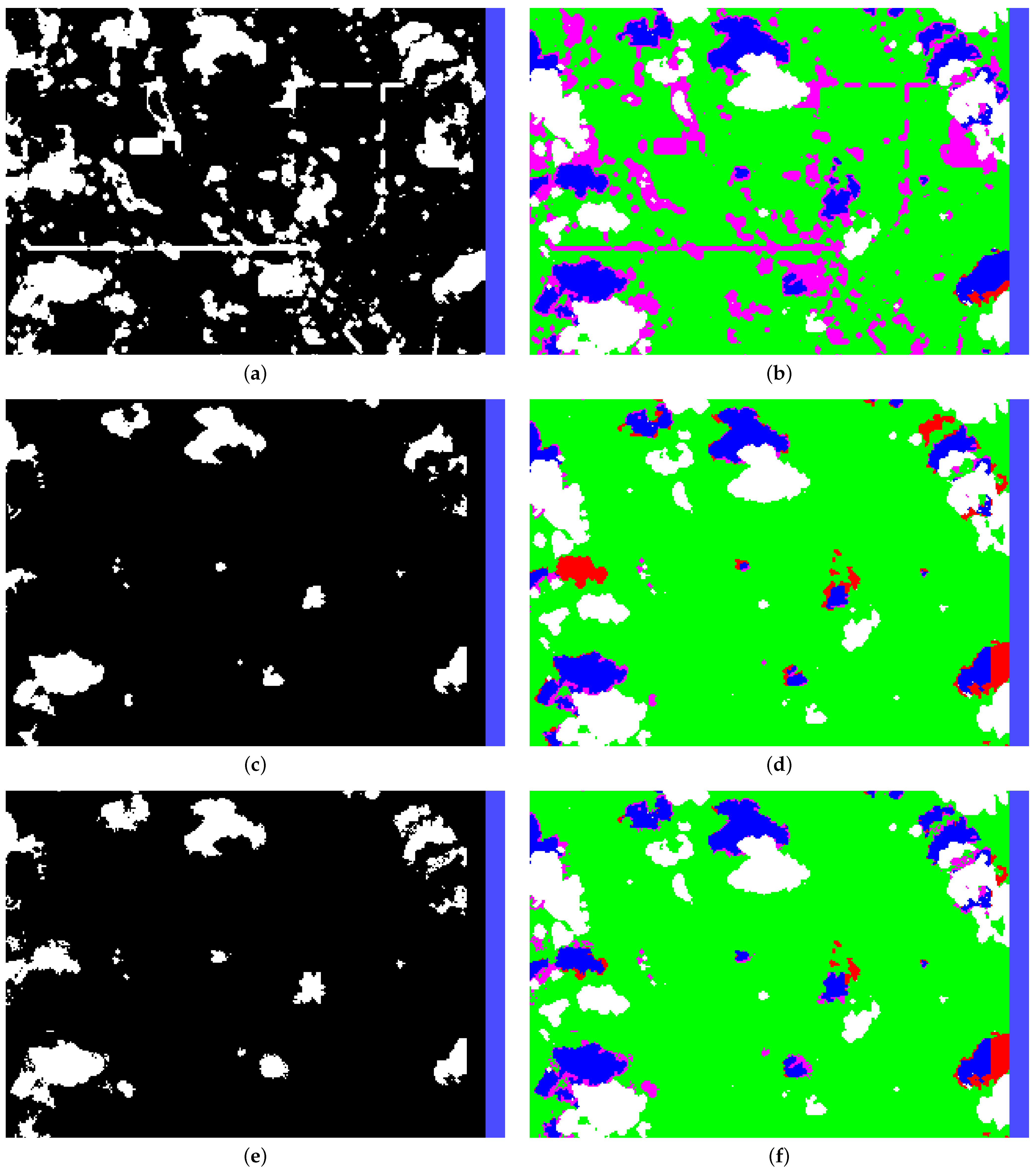For both, a percentage of $100\%$ means no false negatives exist or no false positives to exist. Lastly, since some cloud shadows in the data are a result of clouds outside the image bounds, we added a restriction to the evaluation region. An example of this can be see as a purple line in Figure 9b, which indicates that the bottom and right edges of the image were not included. Without this restriction, the false negative number would increase, reducing the quality of our quantitative error metrics. This can be observed in Appendix B, Figure A3c–f, where the cloud clipping the lower right side is projected properly but with a harsh edge bisecting it due to the harsh edge in the corresponding projected shadow probability ($\beta$) values (Figure A2f). The restricted region is determined by averaging the middle 80% of cloud heights in the scene determined in Section 2.2.4 and performing the ray-casting process on the image boundaries. Any pixel outside this transformed image boundary will be ignored.

$$A_{Producers}={\displaystyle \frac{\sum CorrectShadow}{\sum CorrectShadow+\sum FalseNegative}}={\displaystyle \frac{1-E_{F,SP}}{1-E_{FP,SP}}},$$

(4)

$$A_{Users}={\displaystyle \frac{\sum CorrectShadow}{\sum CorrectShadow+\sum FalsePositive}}={\displaystyle \frac{1-E_{F,SP}}{1-E_{FN,SP}}}.$$

(5)

The results for our metrics are detailed in

Table 4. The candidate shadow mask results of the six datasets for the error metrics outlined in Table 3, Equations (4) and (5). The table is split into three sections, one for each normalization factor is used (number of pixels in the entire image or number of shadow pixels in the baseline) and the producer/user accuracy. Under each normalization factor, we have three types of errors used in the metrics, false positives, false negatives, and false pixels.

Date	${\mathit{A}}_{\mathbf{User}}$	${\mathit{A}}_{\mathbf{Producers}}$	${\mathit{E}}_{\mathbf{FP},\mathit{I}}$	${\mathit{E}}_{\mathbf{FN},\mathit{I}}$	${\mathit{E}}_{\mathit{F},\mathit{I}}$	${\mathit{E}}_{\mathbf{FP},\mathbf{SP}}$	${\mathit{E}}_{\mathbf{FN},\mathbf{SP}}$	${\mathit{E}}_{\mathit{F},\mathbf{SP}}$
15 June	21.53%	89.87%	10.09%	0.31%	10.40%	76.61%	2.37%	78.98%
25 June	4.24%	99.75%	9.88%	0.00%	9.88%	95.75%	0.01%	95.76%
27 June	37.55%	96.32%	19.04%	0.44%	19.48%	61.57%	1.41%	62.98%
5 July	31.31%	91.72%	16.34%	0.67%	17.02%	66.80%	2.75%	69.55%
20 July	25.34%	96.47%	15.94%	0.20%	16.14%	73.98%	0.92%	74.90%
22 July	26.14%	98.78%	21.92%	0.10%	22.01%	73.62%	0.32%	73.94%

,

Table 5. The object-based shadow mask results of the six datasets for the error metrics outlined in Table 3, Equations (4) and (5). Format of this table is the same as Table 4.

Date	${\mathit{A}}_{\mathbf{User}}$	${\mathit{A}}_{\mathbf{Producers}}$	${\mathit{E}}_{\mathbf{FP},\mathit{I}}$	${\mathit{E}}_{\mathbf{FN},\mathit{I}}$	${\mathit{E}}_{\mathit{F},\mathit{I}}$	${\mathit{E}}_{\mathbf{FP},\mathbf{SP}}$	${\mathit{E}}_{\mathbf{FN},\mathbf{SP}}$	${\mathit{E}}_{\mathit{F},\mathbf{SP}}$
15 June	68.57%	63.12%	0.89%	1.14%	2.03%	22.44%	28.60%	51.04%
25 June	75.68%	85.92%	0.12%	0.06%	0.18%	21.64%	11.03%	32.67%
27 June	87.46%	57.14%	0.97%	5.09%	6.07%	7.57%	39.61%	47.18%
5 July	83.42%	62.15%	1.00%	3.07%	4.08%	11.00%	33.69%	44.69%
20 July	80.17%	73.41%	1.02%	1.49%	2.51%	15.37%	22.50%	37.87%
22 July	81.69%	65.80%	1.16%	2.69%	3.84%	12.85%	29.81%	42.66%

and

Table 6. The final shadow mask results of the six datasets for the error metrics outlined in Table 3, Equations (4) and (5). Format of this table is the same as Table 4.

Date	${\mathit{A}}_{\mathbf{User}}$	${\mathit{A}}_{\mathbf{Producers}}$	${\mathit{E}}_{\mathbf{FP},\mathit{I}}$	${\mathit{E}}_{\mathbf{FN},\mathit{I}}$	${\mathit{E}}_{\mathit{F},\mathit{I}}$	${\mathit{E}}_{\mathbf{FP},\mathbf{SP}}$	${\mathit{E}}_{\mathbf{FN},\mathbf{SP}}$	${\mathit{E}}_{\mathit{F},\mathbf{SP}}$
15 June	69.69%	80.15%	1.07%	0.61%	1.68%	25.85%	14.72%	40.57%
25 June	67.30%	93.88%	0.20%	0.03%	0.23%	31.33%	4.20%	35.53%
27 June	84.41%	74.50%	1.64%	3.03%	4.67%	12.09%	22.42%	34.51%
5 July	80.41%	78.71%	1.56%	1.73%	3.29%	16.09%	17.87%	33.96%
20 July	74.48%	86.81%	1.67%	0.74%	2.41%	22.93%	10.17%	33.10%
22 July	77.02%	82.88%	1.94%	1.34%	3.29%	19.83%	13.73%	33.55%

. To assist in comparison and discussion,

Table 7. The mean absolute accuracy and mean percentage change in accuracy of each mask for our six datasets. The first three rows represents the mean absolute accuracy for each mask. Per-dataset results can be found in Table 4, Table 5 and Table 6. The last three rows represents the percentage change in the mean accuracy between two shadow masks (specified in the left column) for the data in the first three columns. For conciseness in the table, the mask names of Candidate Shadow Mask, Object-based Shadow Mask, and Final Shadow Mask are shortened to Candidate, Object, and Final, respectively.

Mask(s)	${\mathit{A}}_{\mathbf{User}}$	${\mathit{A}}_{\mathbf{Producers}}$	${\mathit{E}}_{\mathbf{FP},\mathit{I}}$	${\mathit{E}}_{\mathbf{FN},\mathit{I}}$	${\mathit{E}}_{\mathit{F},\mathit{I}}$	${\mathit{E}}_{\mathbf{FP},\mathbf{SP}}$	${\mathit{E}}_{\mathbf{FN},\mathbf{SP}}$	${\mathit{E}}_{\mathit{F},\mathbf{SP}}$
Mean Absolute Accuracy (Table 4, Table 5 and Table 6)
Candidate	24.35%	95.48%	15.54%	0.29%	15.82%	74.72%	1.30%	76.02%
Object	79.50%	67.92%	0.86%	2.26%	3.12%	15.14%	27.54%	42.68%
Final	75.55%	82.82%	1.35%	1.25%	2.59%	21.35%	13.85%	35.20%
Percentage Change in the Mean Accuracy
Candidate to Object	226%	−29%	−94%	679%	−80%	−80%	2018%	−44%
Object to Final	−5%	22%	60%	−45%	−17%	41%	−50%	−18%
Candidate to Final	210%	−13%	−91%	331%	−84%	−71%	965%	−54%

details the mean of each metric per shadow mask stage and the percentage changes in these mean values between stages. As discussed before, while ideally all metrics should be low, false negatives are more problematic in the case of shadow pixel identification, and their respective metrics should be slightly prioritized for minimization.

4. Discussion

As shown by the results reported in Table 7, the overall accuracy of the masks improves through the three stages. The percentage change relative to the total number of pixels and to the shadow pixels in the baseline both decrease. On average, the object-based shadow mask offers an 80% improvement over the candidate mask. The final shadow mask provides a further improvement of 17% compared to the object-based shadow mask. Overall, from the candidate mask to the final mask, there was an improvement of 84%. The total error improvement when metrics were normalized by the number of shadow pixels was similar, being 44%, 18%, and 54%. According to either metric, the total error of the overall image decreases, and thus, the resulting shadow mask quality is increased at every stage.

Comparing the candidate and the object-based results in Table 7, the false positives are significantly lower with a percent change of false positives of 94% and 80% for the total number of pixels and shadow pixels, respectively. These numbers align with expectations, as the candidate mask is deliberately designed to significantly overestimate the number of shadow pixels. During the ray-casting process, we remove shadow pixels from the candidate mask, leading to the elimination of many false positives. However, this action inadvertently results in the removal of some true positives as well. Consequently, there is a modest increase in the absolute number of false negatives (~2%). However, their relative values increase drastically by 679% and 2018% for the total and shadow normalized metrics, respectively. This is primarily due to the over-representation of false positives in the candidate mask. These errors can come from several sources including errors in the cloud mask, incorrectly matching cloud shadows, or a byproduct of our assumptions in the ray casting process, mainly clouds being restricted to a 2D object.

When comparing the object-based and the final results in Table 7, the false negatives in the final results are much lower than in the object-based shadow mask with a drop of 27.54% to only 13.85% on average, a 50% decrease, which is expected. Even though our preference is to minimize the false negatives, this should be obtained without unduly increasing the number of false positives, striking a balance between the two. The total false positives in the final shadow mask are much lower than the original candidate mask with a drop of 74.72% to 21.35% on average, a 71% decrease, as expected. This is slightly worse than the object-based result of 15.14%, an 80% decrease, but given the false negative error of 27.54% at this stage, the result did not fit our criteria of prioritizing false negatives over false positives, and thus, the post-probability mask offers the best result out of the three masks analyzed.

We compared our results to those reported by Zhu and Woodcock in their 2012 paper, where the producer and user accuracy metrics were used [11]. Their method achieved an average producer accuracy of over 70% and an average user accuracy of approximately 50%. Their algorithm is designed for a much larger set of potential scenes with snow and water detection integrated in the algorithm; however, our post-probability shadow mask significantly improves upon their method. This is demonstrated by our algorithm having an average producer and user accuracy of 82.82% and 75.55% respectively. To evaluate the improvement due to the probability analysis, we evaluated the progression of pixels that were added to the final shadow mask and shadow pixels that were not added to the final shadow mask (Figure 14). We found that the probability analysis correctly added 1.13% of the image’s pixels to the final shadow mask, whereas 0.53% of the image’s pixels were incorrectly added, resulting in a net increase in shadow mask accuracy. However, 1.71% of the image’s pixels were shadow pixel and were not added to the final shadow mask (~60% of possible shadow pixels to add). Looking at the these pixels in Figure 14, 0.34% of the image pixels were incorrectly skipped by the probability analysis were also not present in the potential shadow mask. Since the potential shadow mask overestimates the shadow pixels, these 0.34% pixels are likely to contain pixels that were incorrectly labeled as shadows in the baseline due to human error. Additionally, if we compare our object-based shadow mask to Zhu and Woodcock’s results, we notice that our producer accuracy is similar, being only 67.92%. However, our object-based shadow mask user accuracy is much better at 79.50% already and only reduces about 5% in the final shadow mask. The disparity between the user accuracy may be a result of their algorithm buffering their Fmask, which includes their resulting shadow mask, “by 3 pixels in 8 interconnected directions for each of the matched cloud shadow pixels to fill those small holes” [11]. This results in a low user accuracy due to all the extra pixels added to the edges of detected cloud shadows. Due to the improvement in both the producer and user accuracy of our final result, we conclude that replacing Zhu and Woodcock’s shadow pixel buffer with our proposed statistical model improves the accuracy of the shadow mask output.

Examining the output of our algorithm, it is evident that thin stratus or “wispy” clouds are a conspicuous source of error, as they often produce faint shadows that are difficult to detect for our algorithm. An example of missing cloud shadows for these types of clouds can be seen in Figure 15. The metrics for this scene contains the lowest producer accuracy in Table 5 and Table 6 compared to the other test scenes. Zhu and Woodcock encountered similar issues with their method and noted that their algorithm “may fail to identify a cloud if it is both thin and warm” [11]. Fortunately, often the shadows of these clouds tend to have a smaller impact on the data when missed when compared to thicker and less “wispy” clouds.

Since we use a wide range of heights to test each cloud, clouds will sometimes incorrectly identify the optimal shadow projection and attribute them to other cloud shadows, particularly when the incorrect shadow is larger than the correct shadow. However, as a consequence of the influence distance, the probability analysis often corrects such issues since nearby clouds being correctly projected will inadvertently project the incorrect cloud’s projected shadow probability ($\beta$) values. An example of this is included in Appendix B, Figure A3d, on the left side, where a cloud was missed (seen in red), and Figure A3f, where the cloud was recognized (seen in mostly blue).

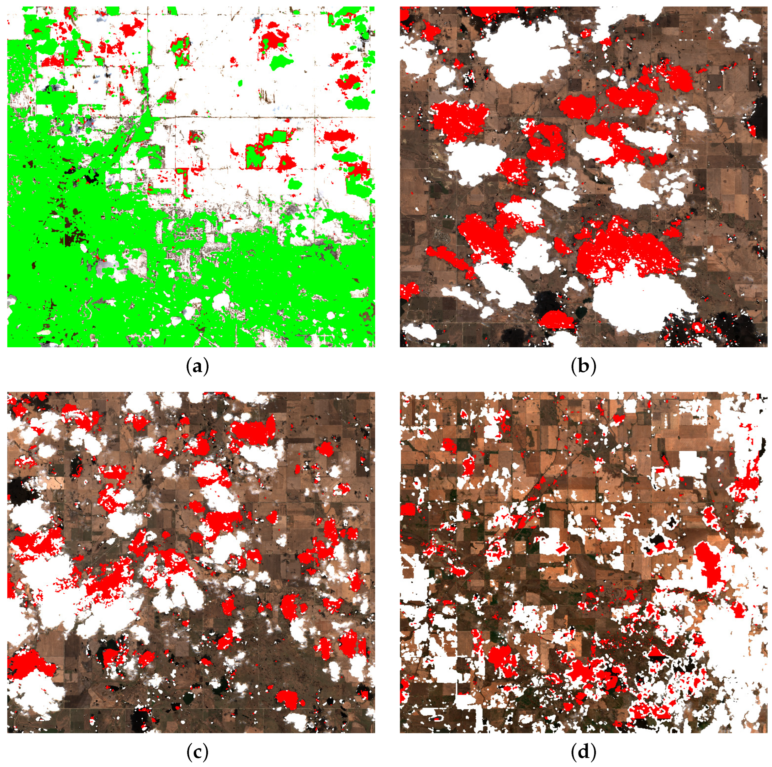
Our method works well in the time periods critical for farmland analysis, the focus of our research; however, evaluating our method outside these times helps to determine the viability or our method for year round analysis, particularly when snow is present, and highlight possible directions for future work. As such, several alternate sets outside the growth season were chosen to qualitatively assess the method’s effectiveness in other seasons. It was found that in the spring/fall season with no snow and dominated by brown vegetation, the result sometimes yields satisfactory results. Specifically, the sets that effectively generated a cloud and shadow mask were 16 April 2020 (Figure 16b) and 1 May 2020 (Figure 16c). 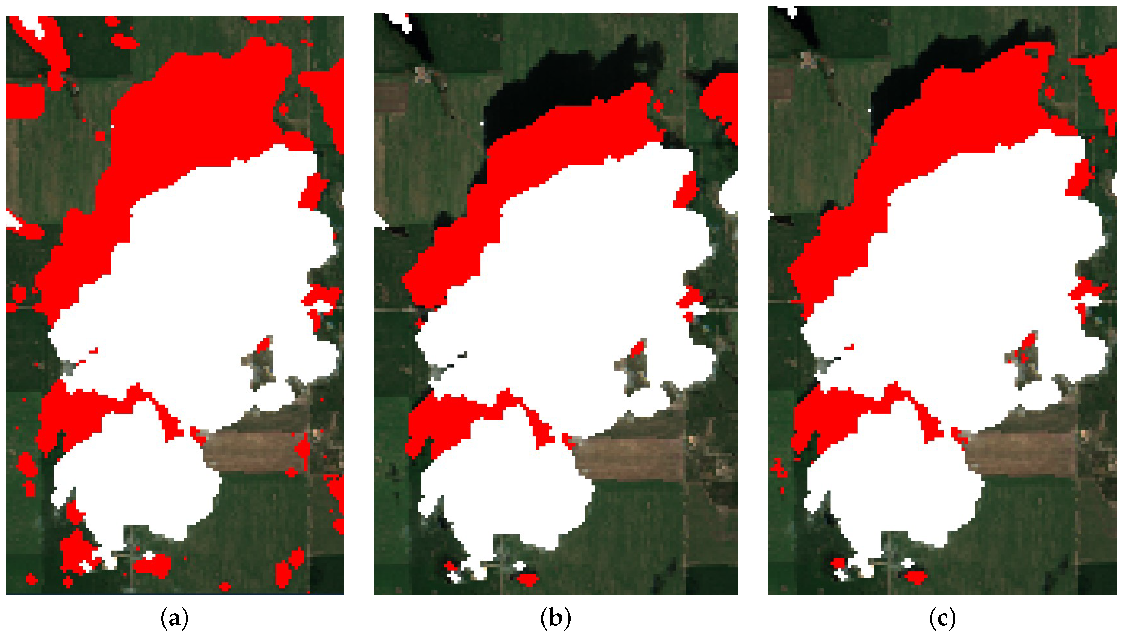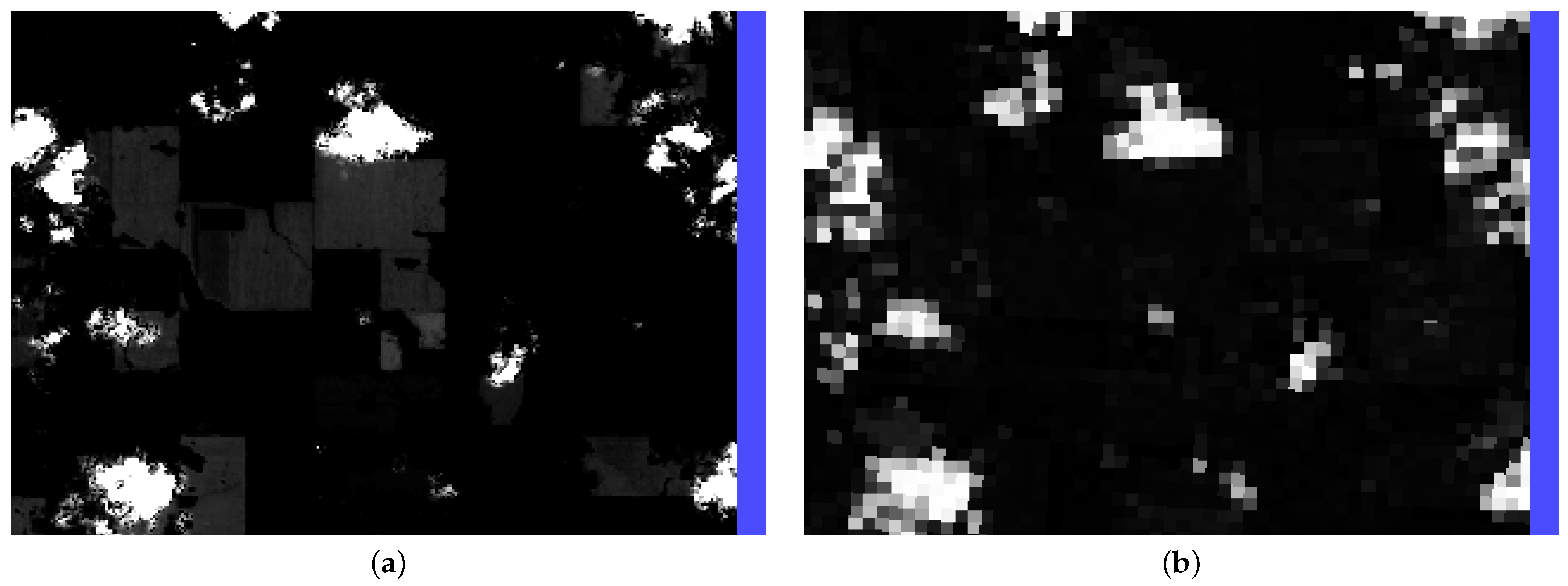However, the proposed method is less successful for datasets 11 April 2020 (Figure 16a) and 15 October 2020 (Figure 16d). In these two examples, the generated cloud mask is poor with excessive false positive cloud pixels, and thus, further processing generates poor shadow masks. In analyzing the snow dataset (11 April 2020), we found that errors in the cloud mask are likely due to poor cloud probability values (too high) generated by Sentinel-2 in CLP₂ (Figure 17b) in the bottom half of the image. However, CLP₁ (Figure 17a) seems correct. The same issue persisted in the 15 October 2020 dataset, though to a lower degree. There may also be a slight problem with CLP₁ (Figure 17c) by inspection. As such, errors in out-of-season data processing are mainly attributed to cloud mask generation.

One assumption made in the methodology similar to Zhu and Woodcock’s method [13] was that clouds are considered as 2D objects. However, for larger cumulus and cumulonimbus clouds, this representation could be less accurate due to the vertical profile of the clouds. Therefore, when the 2D representation is projected, it is missing the elongated portion of the shadow corresponding to the vertical profile. This is evident in Figure 18 from the 27 June 2020 dataset. Through visual inspection, it becomes evident that the subject cloud exhibits a non-negligible vertical component, as observed from the fact that the shadow profile extends beyond the cloud profile. In the potential shadow mask, this extended portion is appropriately identified, which is consistent with expectations. However, in the object-based shadow mask, this extended section is absent due to the lack of overlapping pixels within the projected shadow from the 2D representation, which is absent of a vertical contribution. Although the final shadow mask partially addresses this concern, it remains insufficient in fully rectifying the issue. The other simplifications of zero Earth curvature (flat surface), single view/Sun position, and fixed height of the view/Sun position had no noticeable effects at the given scale.

Limitations and Future Work

The results reported in the previous section illustrate the potential of our method for cloud shadow detection. Nonetheless, manually generating baselines is time-consuming, limiting the number of tests performed. A further study using larger sample size would increase the confidence of the result and possibly allow for further algorithmic optimizations, in particular, the choice of method parameters. We also note that manually generating baselines is a potential source of error.

As discussed previously, this method was developed for a subset of the total possible images Sentinel-2 produces and excludes scenes containing large amounts of water, snow, ice, and dense urban areas. Since water has a low NIR reflectivity, water is included in the potential shadow mask during the pit-filling process, thereby introducing false positives into the candidate mask. As a result, the ray-casting process may select the wrong region as a cloud’s shadow, introducing false negatives by missing the correct shadow. As for snow, ice, and dense urban areas, further testing is required to identify the efficacy of the algorithm for these conditions. Directly incorporating the snow/ice band provided by Sentinel-2 would provide a means to account for images containing snow and ice in our method. For more persistent features, such as bodies of water and urban areas, modifying the method to utilize prior knowledge has the potential to improve the results for data containing such features. Our qualitative analysis suggests that one problem is generating an accurate cloud mask from the cloud probability bands in out-of-season contexts. It appears that improving the cloud mask generation process may substantially reduce the current errors in these contexts. Such extensions are appealing, as they would allow this method to be applied in other contexts aside from farmland analysis.

An extension of the probability analysis could be to use the final shadow mask as input to the ray-casting process for further improvement. This would facilitate an iterative approach, where repeating the ray casting could be used to further improve the results. Similarly, a more complex design of the shadow probability distance factor function, such as utilizing eigenanalysis of the cloud contour (shape), could improve the quality of the generated shadow probability. A further study on the sampling process for the conditional probability function to generate a more accurate statistical model may also be beneficial.

One simplification made by our method was the assumption that clouds can be represented as a planar object to integrate the inverse texture mapping technique for speeding up the ray-casting process. However, clouds with larger vertical components produce a shadow that extend past the shape of the cloud captured from the satellite’s perspective and are often missed. Improving the accuracy of the geometric representation of the cloud, by introducing a 3D representation of the cloud, would increase the accuracy of the results from the improved projected shadows in the ray-casting process. Representing clouds as 3D objects using voxel data has the added benefit of allowing the ray-casting process to consider the density of the cloud to determine its optical transparency. Such a representation would better capture the projected shadow of clouds, especially those that are thin and produce faint shadows. One method to generate 3D clouds by utilizing a “deep learning-based method [that] was developed to address the problem of modelling 3D cumulus clouds from a single image” [24]. Alternative methods have been developed for generating 3D cloud shapes by generating opacity and intensity image to generate volumetric density data for a voxel representation [25]. Other methods using sketch-based techniques for generating volumetric clouds could be automated to generate our cloud objects [26].

Finally, our algorithm depends heavily on the processes developed by Sentinel Hub to produce the CLP₁, CLP₂, and SCL bands. As such, alternative methods for identifying clouds and the cloud probability map are required to apply the proposed method to data originating from other satellites without equivalent data bands. One possible method is to use Sentinel-2’s data to train a neural network to automatically estimate the CLP₁, CLP₂, and SCL bands given data from a different source.

5. Conclusions

In this paper, we proposed a method for determining cloud shadows via geometric refinement using a fast inverse texture mapping ray-casting process with an additional step using a statistical model to refine the shadow result. Evaluating our results in Table 7, it clearly shows an improvement in pixel classification due to the proposed geometric refinement and the statistical model process. When comparing our producer and user accuracy values with those of Zhu and Woodcock’s related method, we can clearly see an improvement. As such, we can conclude our process successfully refines and produces a higher accuracy cloud shadow mask and improves upon Zhu and Woodcock’s method. With the advancement of our algorithm, agriculture companies in Canada and worldwide can leverage our approach to better recover GIS data from partially cloud- and cloud-shadow-obscured images to increase crop yield. Similarly, our algorithm can be used to identify cloud and cloud shadows in many other applications. With the additional processes described in future work to broaden the effective scenes, our algorithm could be used widely for improving business profits, ecological concerns, and more in many other monitored environments.

References

1. Hedengren, J.D. Lagrange Multipliers and their Applications. 2020. Available online: http://sces.phys.utk.edu/~moreo/mm08/method_HLi.pdf (accessed on 19 September 2022).
2. What Is Remote Sensing and What Is It Used for? Available online: https://www.usgs.gov/faqs/what-remote-sensing-and-what-it-used (accessed on 8 August 2022).
3. Shahbandeh, M. Provincial Crop Production GDP Canada 2020. 2020. Available online: https://www.statista.com/statistics/858240/provincial-crop-production-gdp-canada/ (accessed on 20 September 2021).
4. Ravensberg, S. GIS in Agriculture. 2018. Available online: https://www.integratesustainability.com.au/2018/11/23/gis-in-agriculture/ (accessed on 16 August 2022).
5. Lenhardt, J.; Xu, H. Clean up Your Landsat Imagery: Removing Cloud and Cloud Shadow. Available online: https://www.esri.com/arcgis-blog/products/arcgis-pro/imagery/clean-up-your-landsat-imagery-removing-cloud-and-cloud-shadow/ (accessed on 17 December 2022).
6. Wang, T.; Shi, J.; Letu, H.; Ma, Y.; Li, X.; Zheng, Y. Detection and Removal of Clouds and Associated Shadows in Satellite Imagery Based on Simulated Radiance Fields. J. Geophys. Res. Atmos. 2019, 124, 7207–7225. [Google Scholar] [CrossRef] [Green Version]
7. Ibrahim, E.; Jiang, J.; Lema Vélez, L.; Barnabé, P.; Giuliani, G.; Lacroix, P.; Pirard, E. Cloud and Cloud-Shadow Detection for Applications in Mapping Small-Scale Mining in Colombia Using Sentinel-2 Imagery. Remote Sens. 2021, 13, 736. [Google Scholar] [CrossRef]
8. Gould, R.; Hou, W.; Lee, Z.; Arnone, R. Automated Detection and Removal of Cloud Shadows on HICO Images. Proc. SPIE 2011, 8030, 803004. [Google Scholar] [CrossRef]
9. Jin, S.; Homer, C.; Yang, L.; Xian, G.; Fry, J.; Danielson, P.; Townsend, P. Automated cloud and shadow detection and filling using two-date Landsat imagery in the USA. Int. J. Remote Sens. 2013, 34, 1540–1560. [Google Scholar] [CrossRef]
10. Chai, D.; Newsam, S.; Zhang, H.K.; Qiu, Y.; Huang, J. Cloud and cloud shadow detection in Landsat imagery based on deep convolutional neural networks. Remote Sens. Environ. 2019, 225, 307–316. [Google Scholar] [CrossRef]
11. Zhu, Z.; Woodcock, C.E. Object-based cloud and cloud shadow detection in Landsat imagery. Remote Sens. Environ. 2012, 118, 83–94. [Google Scholar] [CrossRef]
12. Zhu, Z.; Woodcock, C.E. Automated cloud, cloud shadow, and snow detection in multitemporal Landsat data: An algorithm designed specifically for monitoring land cover change. Remote Sens. Environ. 2014, 152, 217–234. [Google Scholar] [CrossRef]
13. Zhu, Z.; Wang, S.; Woodcock, C.E. Improvement and expansion of the Fmask algorithm: Cloud, cloud shadow, and snow detection for Landsats 4–7, 8, and Sentinel 2 images. Remote Sens. Environ. 2015, 159, 269–277. [Google Scholar] [CrossRef]
14. Haines, E. An Introduction to Ray Tracing; Academic Press Ltd.: London, UK, 1989. [Google Scholar]
15. Main-Knorn, M.; Pflug, B.; Louis, J.; Debaecker, V.; Müller-Wilm, U.; Gascon, F. Sen2Cor for Sentinel-2. Proc. SPIE 2017, 3, 10427. [Google Scholar] [CrossRef] [Green Version]
16. Zupanc, A. Improving Cloud Detection with Machine Learning. 2017. Available online: https://medium.com/sentinel-hub/improving-cloud-detection-with-machine-learning-c09dc5d7cf13 (accessed on 26 July 2023).
17. Li, Z.; Shen, H.; Weng, Q.; Zhang, Y.; Dou, P.; Zhang, L. Cloud and cloud shadow detection for optical satellite imagery: Features, algorithms, validation, and prospects. ISPRS J. Photogramm. Remote Sens. 2022, 188, 89–108. [Google Scholar] [CrossRef]
18. Stewart, M. The Limitations of Machine Learning. 2019. Available online: https://towardsdatascience.com/the-limitations-of-machine-learning-a00e0c3040c6 (accessed on 12 September 2021).
19. Sentinel-2 L2A. Available online: https://docs.sentinel-hub.com/api/latest/data/sentinel-2-l2a/ (accessed on 24 July 2023).
20. Sentinal 2 Cloud Masks. Available online: https://docs.sentinel-hub.com/api/latest/user-guides/cloud-masks/ (accessed on 24 August 2021).
21. Erickson, J. Algorithms; Independently Published: Urbana, IL, USA, 2019; pp. 205–207. [Google Scholar]
22. Soille, P.; Vogt, J.; Colombo, R. Carving and Adaptive Drainage Enforcement of Grid Digital Elevation Models. Water Resour. Res. 2003, 39. [Google Scholar] [CrossRef]
23. Li, H. How Many Satellites Are Orbiting the Earth in 2021? 2008. Available online: https://www.geospatialworld.net/blogs/how-many-satellites-are-orbiting-the-earth-in-2021/ (accessed on 28 September 2021).
24. Zhang, Z.; Cen, Y.; Zhang, F.; Liang, X. Cumulus cloud modeling from images based on VAE-GAN. Virtual Real. Intell. Hardw. 2021, 3, 171–181. [Google Scholar] [CrossRef]
25. Dobashi, Y.; Shinzo, Y.; Yamamoto, T. Modeling of Clouds from a Single Photograph. Comput. Graph. Forum 2010, 29, 2083–2090. [Google Scholar] [CrossRef] [Green Version]
26. Stiver, M.; Baker, A.; Runions, A.; Samavati, F. Sketch Based Volumetric Clouds. In Proceedings of the Smart Graphics, 10th International Symposium on Smart Graphics, Banff, AL, Canada, 24–26 June 2010; Krüger, A., Olivier, P., Eds.; Springer: Berlin/Heidelberg, Germany, 2010; pp. 1–12. [Google Scholar]
Figure 1. Image (a) is the chosen study area, detailed in Section 2.1, with clear sky captured on 21 July 2018 [19]. The following insets highlight the diverse features in this Albertan region. (b) The town of Irricana in the upper half, with farmland in the bottom half. (c) The village of Craigdhu in the bottom right, with a large body of water in the center. (d) The village of Beiseker. (e) Some dirt or barren land.
Remotesensing 15 03955 g001aRemotesensing 15 03955 g001b
Figure 2. Overall process for our cloud shadow detection algorithm. Using Sentinel-2 data, we can generate the potential shadow candidate mask, cloud mask, and solve for the best fit Sun and satellite positions. Since the generation of potential shadows depends on detected clouds in the image, the cloud mask is generated first. Before the ray-casting process, we need to partition the cloud mask into distinct cloud objects to individually ray-cast. The ray-casting process is applied to each cloud in the scene to prune the shadow mask of false positives, which is then processed in a statistical model to refine the final shadow mask.
Remotesensing 15 03955 g002
Figure 3. Process flow for generating the cloud mask (a) and the potential shadow candidate mask (b). In the diagrams, the slanted parallelograms indicate image data, the rectangles represent processes applied to the inputs, and the ellipses represent a logical or mathematical operation indicated by the symbol (-) or word (OR, AND, NOT) they contain. The selected mask generation processes applied to the SCL mask indicate which pixel values (IDs indicating a certain pixel type; see Sentinel-2’s documentation [19] for further details) are considered to be true, while all others are considered to be false.
Remotesensing 15 03955 g003
Figure 4. Example demonstrating the impact of boundary conditions on the potential shadow mask. To the left is a manually created example of a grayscale NIR-band image. Inside the image, there are 4 cloud shadows at various strengths. Three cloud shadows intersect with the border, and the last one does not. Each pixel level is indicated by the numbers in the white squares and are in the range [ 0 , 1 ] . Neighboring cells with the same grayscale intensity share the same value. To the right of the image are three rows containing results at various stages, depending on the chosen boundary value, as seen along the top. In the first row, we have the pit-filled NIR result. Note that to illustrate the boundary level better, an additional column to the right of the images is inserted with the intensity of the boundary value. In the middle is the difference between the pit-filled NIR and original. At the bottom is the result of applying a threshold of 0.12 to the difference band. As the boundary value is increased, more pixels are added to the threshold result. If the threshold is too low, many non-shadow pixels of clouds intersecting with the boundary are missed; however, note that the cloud in the middle of the image is identified correctly, even with a boundary value of 0. If the boundary value is too high, many pixels will be added to the shadow mask, highlighted when the boundary value is 0.95. Comparing the original NIR to the shadow mask, a boundary value of 0.7 produces the best result as it is closest to the clear-sky value of the NIR band, 0.8.
Remotesensing 15 03955 g004
Figure 5. Example output for the cloud and potential candidate shadow. (a) The original RGB band. (b) Combined cloud and candidate mask overlaying RBG band. Candidate shadows are shown in red, clouds are shown in white, and all other pixels retain their original RGB values. The dataset is from 20 July 2020.
Remotesensing 15 03955 g005
Figure 6. An example least squares problem (Equations (1) and (2)) on a 4 by 3 grid (image). Each cell, with P i at the center, has a direction vector, d ^ i , that defines a line connecting the convergence point and P i defining a perspective projection. The optimal convergence point, X, that minimizes the distance to all perspective lines at a given height, h.
Remotesensing 15 03955 g006
Figure 7. Visual depiction of the ray-casting process in a single iteration. The lower plane represents the ground. The upper plane is parallel to the ground, situated at height h. The Sun and Sentinel-2 satellite are seen at the top in green and red, respectively. Following the projection lines to Sentinel-2, Q c is projected onto the height plane to produce Q i . Following the projection lines from the Sun, Q i is projected to the ground to produce Q s .
Remotesensing 15 03955 g007
Figure 8. Example output for the object-based shadow mask. (a) The original RGB band. (b) The object-based shadow mask overlaid into the RGB band. Red pixels represent cloud shadows and white pixels represent clouds. Around several selected example clouds and their respective shadows are boxes representing Q c (yellow) and Q s (turquoise), respectively. The dataset is from 20 July 2020.
Remotesensing 15 03955 g008
Figure 9. Example output for the shadow projected probability map: (a) The original RGB band; (b) The projected shadow probability mask generated for the 20 July 2020 dataset. Like in Figure 8, we can see several Q c (yellow) and Q s (turquoise). In addition to this, there is a purple box indicating the valid evaluation zone as a result of the boundary clouds identified during the ray-casting process ( Section 3). The whiter the pixels are, the higher β is. As seen in the figure around each cloud, there is a smooth falloff due to the distance scaling and the probabilities do extend past the Q s bounding boxes.
Remotesensing 15 03955 g009
Figure 10. Construction of the probability surface f ( α , β ) . Image (a) is a 3D view of the probability surface construction problem. We have α and β along the horizontal axes, with f ( α , β ) along the vertical axis. The red and blue data points correspond to pixels with their α and β values from the shadow value map and the shadow probability projection map, respectively. Red data points correspond to pixels not in shadow in the object-based shadow ( f ( α , β ) = 0 ), while blue data points correspond to pixels in shadow ( f ( α , β ) = 1 ). Image (b) is a cross section of the desired probability surface. Note that the surface is approximating and not interpolating the given data points.
Remotesensing 15 03955 g010
Figure 11. The probability surface visualized as a triangular mesh from the 20 July 2020 dataset. Along the bottom are the α and β axes ranging from 0 to 1. Along the left side is the f ( α , β ) axis, again ranging from 0 to 1. At the f ( α , β ) = 0.15 height, we have a semitransparent plane that indicates the probability cutoff to determine if a pixel should ( f ( α , β ) 0.15 ) or should not ( f ( α , β ) < 0.15 ) be added to the final shadow mask.
Remotesensing 15 03955 g011
Figure 12. Example output for the final shadow mask. (a) The original RGB band. (b) The final shadow mask generated for the 20 July 2020 dataset. The color scheme is the same as Figure 8. Note that the shadows are extending past the original Q s bounding boxes.
Remotesensing 15 03955 g012
Figure 13. Example shadow baseline used for method evaluation (a) with the RBG image (b) for comparison. The baseline is displayed on the NIR band provided by Sentinel-2 with green pixels indicating shadows. The dataset is from 20 July 2020.
Remotesensing 15 03955 g013
Figure 14. Bar graph illustrating the impact of the probability analysis on shadow pixel classification. Pixels used for the plot fall in three categories: shadow pixels that were missed by the object-based shadow mask, but added to final the shadow mask (left); shadow pixels that were missed by the object-based shadow mask and are also absent from the final shadow mask (middle); and non-shadow pixels that were omitted from the object-based shadow mask but were added to the final shadow mask (right). Each bar is divided into two groups depending on whether the object-based shadow mask changed the pixel’s classification. Percentages indicate the average percent of all pixels. Labels of the form B-XYZ use 4 binary labels (T/F) to indicate the classification of each pixel in the shadow baseline (B), potential shadow mask (X), object-based shadow mask (Y), and final shadow mask (Z, following probability analysis). For example, a shadow pixel that was incorrectly classified in the potential and object shadow masks and corrected by our probability analysis would be labeled T-FFT.
Remotesensing 15 03955 g014
Figure 15. Image of scene depicted in the 27 June 2020 dataset. See the bottom right side of the image for the high volume of thin stratus or “wispy” clouds, causing a decrease in the producer accuracy as seen in Table 5 and Table 6.
Remotesensing 15 03955 g015
Figure 16. Off-season examples of the method’s performance. Each panel depicts an RGB image for a different date, overlaid with the final shadow mask (red) and cloud mask (green for (a) and white for others). The data for each panel are as follows: (a) 11 April 2020, a landscape with significant snow cover (especially top right region); (b) 26 April 2020, an early spring season conditions with mostly brown vegetation; (c) 1 May 2020, which has similar characteristics to (b); and (d) 15 October 2020, fall season conditions with mostly brown vegetation.
Remotesensing 15 03955 g016
Figure 17. In images (a,b), we have CLP1 and CLP2 from 11 April 2020 dataset (Figure 16a). Similarly, (c,d) are from the 15 October 2020 dataset (Figure 16b). For all images, the brighter the pixel is, the larger probability of a cloud being present is.
Remotesensing 15 03955 g017
Figure 18. A set of images demonstrating the effect of representing clouds as 2D objects. Each of these images are taken from a subset of the 27 June 2020 dataset, focusing on a particular cloud in white and its corresponding shadow in red. Each image is from a shadow mask: (a) the potential shadow mask, (b) the object-based shadow mask, and (c) the final shadow mask.
Remotesensing 15 03955 g018