Multi-Objective Multi-Satellite Imaging Mission Planning Algorithm for Regional Mapping Based on Deep Reinforcement Learning

Abstract

Satellite imaging mission planning is used to optimize satellites to obtain target images efficiently. Many evolutionary algorithms (EAs) have been proposed for satellite mission planning. EAs typically require evolutionary parameters, such as the crossover and mutation rates. The performance of EAs is considerably affected by parameter setting. However, most parameter configuration methods of the current EAs are artificially set and lack the overall consideration of multiple parameters. Thus, parameter configuration becomes suboptimal and EAs cannot be effectively utilized. To obtain satisfactory optimization results, the EA comp ensates by extending the evolutionary generation or improving the evolutionary strategy, but it significantly increases the computational consumption. In this study, a multi-objective learning evolutionary algorithm (MOLEA) was proposed to solve the optimal configuration problem of multiple evolutionary parameters and used to solve effective imaging satellite task planning for region mapping. In the MOLEA, population state encoding provided comprehensive population information on the configuration of evolutionary parameters. The evolutionary parameters of each generation were configured autonomously through deep reinforcement learning (DRL), enabling each generation of parameters to gain the best evolutionary benefits for future evolution. Furthermore, the HV of the multi-objective evolutionary algorithm (MOEA) was used to guide reinforcement learning. The superiority of the proposed MOLEA was verified by comparing the optimization performance, stability, and running time of the MOLEA with existing multi-objective optimization algorithms by using four satellites to image two regions of Hubei and Congo (K). The experimental results showed that the optimization performance of the MOLEA was significantly improved, and better imaging satellite task planning solutions were obtained.

1. Introduction

The regional image products obtained through satellite remote sensing are essential spatial data in the digital development of the region [1,2,3]. However, although remote sensing image processing has been widely researched for region mapping [4,5,6], limited studies have focused on satellite image acquisition technology. Therefore, the acquisition times of regional images have remained long, and periodic production remains difficult because precious satellite resources cannot be efficiently utilized. Imaging satellite mission planning is a crucial technology for improving the efficiency of satellite image acquisition [7]. Imaging benefits are maximized by appropriately adjusting satellite observation targets at suitable times according to user requirements, satellite attribute information, and relevant constraints, such as energy, mobility, and storage constraints. However, numerous contradictions exist between user requirements and imaging satellite performance. Therefore, trade-offs exist in imaging satellite mission planning, which is a complex multi-objective optimization problem [8].

Numerous multi-objective evolutionary algorithms [9] have been proposed to achieve valuable results, such as many-objective optimization [10], large-scale multi-objective optimization [11], and parameter configuration [12]. With the development of evolutionary algorithms, parameter configuration has become critical in evolutionary computing because the performance of EAs depends considerably on their parameters [13]. However, it was often ignored because the sub-optimal parameter configuration can be compensated by prolonging the evolutionary generation and improving the evolutionary strategy. The parameter configuration methods are categorized into parameter tuning and parameter control. Parameter tuning refers to determining fixed parameter values for EAs before it runs. Manual adjustment is the most common method for parameter tuning [14,15]. Parameter tuning is mature and widely used in industry and academia. However, regardless of optimizing the parameter tuning method, a common shortcoming is as follows: the static parameter setting contradicts EAs, which is a dynamic process. Thus, the optimization performance of the EAs is limited.

Parameter control is a parameter configuration method in which the parameters change with the evolution process to improve algorithm performance. According to various parameter control methods, parameter control can be categorized into deterministic and adaptive parameter control.

Deterministic methods [16] are uninformed, i.e., population feedback information is not considered during the parameter selection. A time-varying function controls parameter selection in a deterministic method, such as the sigmoid [17] and piecewise functions [18]. Aiming at the parameter sensitivity problem of MOEA, Dai [19] proposed a deterministic MOEA framework based on collaborative granular sieving. The proposed method automatically selected evolutionary parameters guided by mathematical principles to guarantee convergence to the global optimal solution.

In adaptive parameter control [20,21], the magnitude and direction of evolution parameters are determined based on the partial feedback information. For example, in [22], instead of reference vectors, the optical solutions and normal-boundary directions were used to guide the population to adapt to the shape of the Pareto front automatically. In [23], an MOEA was proposed based on a self-adaptive crossover operator and interval initialization. Instead of the adaptive crossover rate, the proposed MOEA-ISa can dynamically determine the number of non-zero genes in offspring based on the similarity degree of parents. In [24], selection pressure was adapted by encoding the size of the tournament in the genome.

In recent years, some scholars used reinforcement learning (RL) [25] for parameter control. In this method, evolutionary parameters were selected through the feedback information of the population state, which is not affected by evolutionary strategies. Therefore, this method is a general parameter control method. In [26], the time difference algorithm was used to map the fitness value to evolutionary parameters (population size, competitive selection ratio, crossover rate, and mutation rate) by a Q table. However, because of the limitations of RL, only discrete small-scale optimization problems can be solved, and this method cannot be adapted to the continuous changes in evolutionary parameters. Therefore, the parameter control based on RL is not feasible. Deep reinforcement learning (DRL) [27] has been developed as a novel approach to overcome this problem. For example, Schuchardt uses DRL to solve the problem of single-parameter configuration for single objective functions [28]. Kaiwen transformed the multi-objective discrete problem into multiple single-objective discrete problems and then optimized these single-objective functions by DRL [29]. To solve the problem of sensitive parameter configuration of EAs, Song [30] proposed a genetic algorithm based on RL (RL-GA). In RL-GA, Q-learning was used for selecting crossover and mutation operations. Similarly, Tian [31] proposed a multi-objective optimization algorithm MOEA-DQN based on a deep Q network to solve the adaptive operator selection problem. In MOEA-DQN, four different mutation operators were used as candidate operators for different population states. Reijnen [32] proposed a differential evolutionary (DE) algorithm based on DRL and parameter adaptive control, called DRL-APC-DE. The mutation parameters of the DE are adaptively controlled through DRL. To solve the scheduling problem of continuous annealing operations in the steel industry, Li [33] proposed an adaptive multi-objective differential evolutionary algorithm based on DRL, called AMODE-DRL. The AMODE-DRL can adaptively select mutation operators and parameters according to different search domains.

Although adaptive parameter configuration has been studied extensively, the following problems persist: first, the existing parameter control is based on a single parameter or a combination of multiple single parameters, which lacks the consideration of multiple parameters simultaneously. Furthermore, complex interactions exist among various parameters, and these influences are difficult to describe with mathematical expressions [13]. Second, evolutionary parameter configuration typically obeys the artificially set change rules or uses part of the population information. It results in the population information not accurately guiding the setting of evolutionary parameters, i.e., the parameter setting is sub-optimal. Third, the generality and robustness of the algorithm are unsatisfactory. The parameters of the same algorithm should be reconfigured for various application problems. Limited studies have focused on evolutionary parameter configuration methods based on DRL, configuring multiple evolutionary parameters simultaneously, adapting to continuous and discrete problems simultaneously, and general applicability to most MOEAs.

This study proposed a novel multi-objective learning evolutionary algorithm (MOLEA) based on DRL for satellite imaging task planning for regional mapping. The MOLEA maximizes the evolutionary benefits through DRL, thereby maximizing the optimization efficiency of the proposed algorithm. Specifically, the contribution of this study is summarized as follows:

(1)

The scene data for fast training were constructed. For imaging satellite mission planning, the calculation is complex, and its efficiency is low, which results in a slow training speed for directly using the mission planning model as the training scene data. The easy-to-calculate public test functions were constructed as the same structure as the task planning model and then used as training scene data to improve the efficiency of algorithm training.

(2)

Hypervolume (HV) was first proposed as a multi-objective evolutionary reward to guide the evolution of MOEA. As a scalar, HV makes it possible to apply DRL to MOEAs and enables the convergence and distribution of MOEAs to guide evolution simultaneously.

(3)

The MOLEA was proposed. The MOLEA obtains all the population state information of each generation of the population through population state coding, which is used to guide the setting of evolutionary parameters. A simple neural network was used to map the relationship between population state information and multiple evolutionary parameters without determining its influence relationship. Through training, the parameter setting of each generation exhibits the maximum evolutionary benefit for improving the optimization performance of the algorithm.

(4)

The effectiveness of the proposed MOLEA in imaging satellite mission planning was verified by comparing the MOLEA with four classical MOEAs. Experimental results revealed that the MOLEA considerably improves optimization efficiency and affects imaging satellite mission planning.

The rest of this paper is organized as follows. Section 2 briefly introduces the multi-satellite imaging task planning model for region mapping. Section 3 details the procedure of the proposed MOLEA. Section 4 presents the experimental results and analysis of the MOLEA and comparison algorithms. Finally, the discussion and conclusion are presented in Section 5 and Section 6, respectively.

2. Multi-Satellite Mission Planning Model for Regional Mapping

We used the model in [34] for the multi-satellite imaging mission planning for area mapping as follows:

(1)

Decision variables:

$$y_{ki}=\left\{\begin{array}{l}1, \mathrm{if} \mathrm{the} \mathrm{strip} x_{ki}\mathrm{participates} \mathrm{in} \mathrm{imaging}\\ 0, \mathrm{otherwise}\end{array}\right.$$

(1)

$$x=(x_{11},x_{12},\cdots x_{ki}\cdots ,x_{Kn})$$

(2)

where $y_{ki}$ indicates whether the strip with satellite swing angle $x_{ki}$ participates in regional imaging. If so, $y_{ki}=1$; otherwise, $y_{ki}=0$. And $x$ represents the set of swing angles for each imaging of the satellites, and its length is $M$. Furthermore, $x_{ki}$ represents the imaging swing angle when satellite $k$ passes the target area for the $i$-th time.

(2)

Objective functions:

$$\min f\left(x\right)=1-\frac{S_{\mathrm{cov}}\left(x\right)}{S_{obj}}$$

(3)

$$\min g\left(y_{ki}\right)={\displaystyle \sum _{i=1}^M{y}_{ki}}/M$$

(4)

where (3) ensures the maximum coverage of the imaging area. $S_{\mathrm{cov}}\left(x\right)$ is the effective coverage area of all imaging strips, and $S_{obj}$ is the target area. Equation (4) ensures the least number of satellite imaging, i.e., the least consumption of satellite resources.

(3)

Constraint conditions:

$$06:00\le T_{\mathrm{local}}\le 18:00$$

(5)

$$x_{\min }\le x_{ki}\le x_{\max }$$

(6)

where (5) indicates that the optical satellite satisfies the daytime imaging constraints, and (6) indicates the maneuverability of satellite $k$. $x_{\min }$ and $x_{\max }$ are the minimum and maximum swing angles of the satellite, respectively.

The multi-satellite imaging mission planning model used in this study is a real binary mixed coding multi-objective optimization problem.

3. Proposed MOLEA

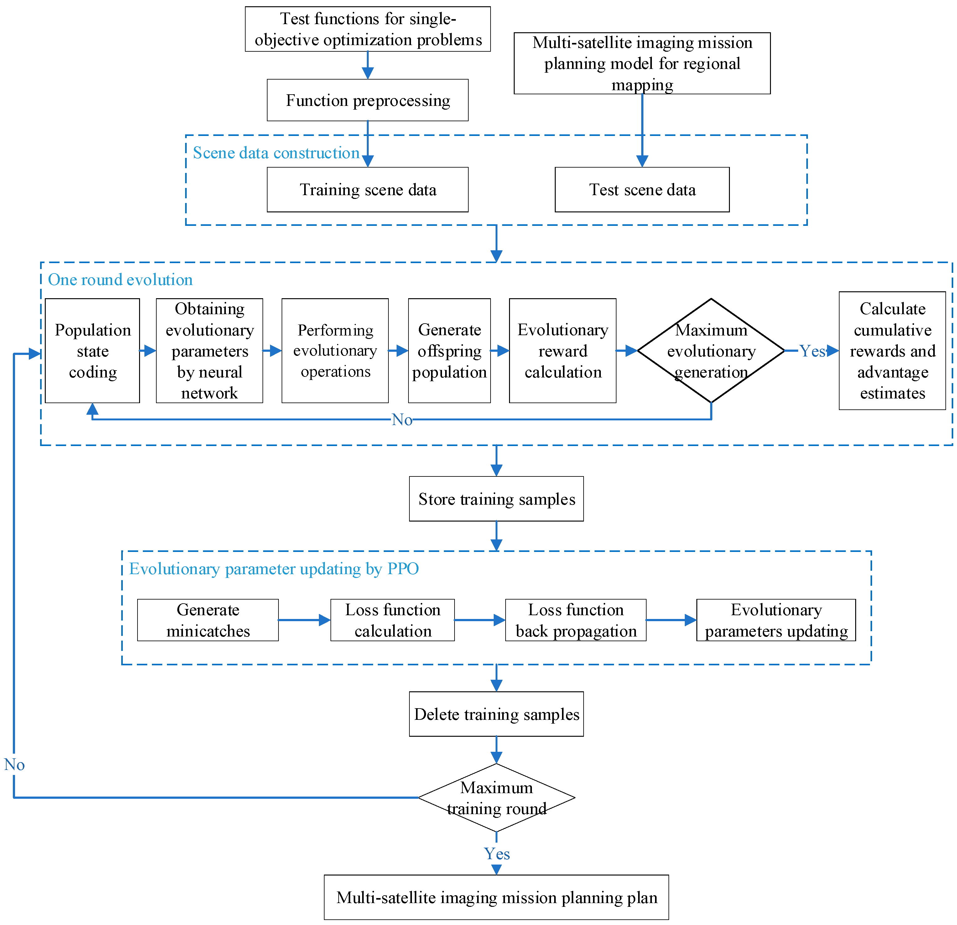
3.1. MOLEA Framework

The MOLEA framework is displayed in Figure 1. The framework includes three core parts. First, scene data are constructed for fast training based on the public single-objective test function. Second, N-generation evolution is performed. This step is similar to the conventional evolution process. The difference is that evolutionary parameters are obtained by population state coding and neural network, and the evolutionary parameters need to be evaluated by calculating evolutionary reward, cumulative reward, and advantage estimation. Third, the evolutionary parameters are updated by proximal policy optimization (PPO) [35] based on the obtained training samples until the evolutionary parameter configuration with the greatest benefit is obtained.

3.2. Scene Data Construction for Fast Training

As we all know, the agent and the environment need to interact many times for DRL to generate sufficient training samples. Therefore, the mission planning model needs to be calculated numerous times. However, the mission planning model calculation involves region information, satellite orbit information, and complex imaging geometric operations. It is complex and inefficient. Therefore, there is a slow training speed by directly using the task planning model as the training scene data.

A novel method is proposed to construct scene data based on the task planning model in Section 2 to improve the training speed. In this method, seven single-objective test functions with multi-dimensional decision variables are selected. Then, these functions are reconstructed through normalization and multi-objective transformation to have the same structure as the task planning model. The redeveloped functions are used as training scene data. The seven single-objective test functions are as follows: Griewank, rotated hyper-ellipsoid, quartic, Rastrigin, Rosenbrock, sphere, and Styblinski–Tang functions [36,37]. The multi-dimensional decision variables correspond to multiple imaging strips in the mission planning model. Normalization makes the value of $obj1$ changes within [0, 1], which corresponds to the first objective function of the task planning model. The multi-objective transformation adds a function $obj2$ to $obj1$, which corresponds to the second objective function of the task planning model. $obj2$ determines the decision variables involved in calculating $obj1$. The scene data constructed are as follows:

• Improved Griewank function:

$$\left\{\begin{array}{l}obj1=\frac{1}{\max }\left({\displaystyle \sum _{i=1}^d\frac{x_i^2}{4000}-{\displaystyle \prod _{\mathrm{i}=1}^d\cos \left(\frac{x_i}{\sqrt{i}}\right)+1}}\right)\\ obj2=\frac{{\displaystyle \sum _{i=1}^d{y}_i}}{d}\end{array}\right.$$

(7)

• Improved rotated hyper-ellipsoid function:

$$\left\{\begin{array}{l}obj1=\frac{1}{\max }\left({\displaystyle \sum _{i=1}^d{\displaystyle \sum _j^i{x}_j^2}}\right)\\ obj2=\frac{{\displaystyle \sum _{i=1}^d{y}_i}}{d}\end{array}\right.$$

(8)

• Improved quartic function:

$$\left\{\begin{array}{l}obj1=\frac{1}{\max }\left({\displaystyle \sum _{i=1}^{n}i{x}_i^4+random[0,1)}\right)\\ obj2=\frac{{\displaystyle \sum _{i=1}^d{y}_i}}{d}\end{array}\right.$$

(9)

• Improved Rastrigin function:

$$\left\{\begin{array}{l}obj1=\frac{1}{\max }\left(10d+{\displaystyle \sum _{i=1}^d[x_i^2-10\cos (2\pi x_i)]}\right)\\ obj2=\frac{{\displaystyle \sum _{i=1}^d{y}_i}}{d}\end{array}\right.$$

(10)

• Improved Rosenbrock function:

$$\left\{\begin{array}{l}obj1=\frac{1}{\max }\left({\displaystyle \sum _{i=1}^{d-1}[100{(x_{i+1}-x_i^2)}^2+{(x_i-1)}^2]}\right)\\ obj2=\frac{{\displaystyle \sum _{i=1}^d{y}_i}}{d}\end{array}\right.$$

(11)

• Improved sphere function:

$$\left\{\begin{array}{l}obj1=\frac{1}{\max }\left({\displaystyle \sum _{i=1}^d{x}_i^2}\right)\\ obj2=\frac{{\displaystyle \sum _{i=1}^d{y}_i}}{d}\end{array}\right.$$

(12)

• Improved Styblinski–Tang function:

$$\left\{\begin{array}{l}obj1=\frac{1}{\max }\left(\frac{1}{2}{\displaystyle \sum _{i=1}^d(x_i^4-16x_i^2+5x_i)}\right)\\ obj2=\frac{{\displaystyle \sum _{i=1}^d{y}_i}}{d}\end{array}\right.$$

(13)

The constructed scene data exhibit the same structure as the task planning model and the same value range of decision variables and objective functions. Compared to the task planning model, the proposed constructed scene data calculation is simple and efficient. It effectively improves the training efficiency when the objective function requires many calculations.

3.3. Evolutionary Operations Based on DRL

The primary purpose of this section is to generate training samples for updating evolutionary parameters by performing evolutionary operations repeatedly. The training samples include the population state $s_t$ of the $t$-th generation, evolutionary parameters of the $t$-th generation, new population state $s_{t+1}$ reached, evolutionary reward $R_t$, cumulative reward $V(s_t)$, and advantage estimate $\widehat{A}(t)$. In our research, the number of obtained training samples is the number of training scenes (7) × the number of optimizations for each training scene (4) × the evolutionary generation for each optimization (100) × the total number of training iterations (500). The samples are obtained through the following steps.

3.3.1. Population State Coding

In order for the population information to fully influence the evolutionary parameters, the population state is encoded before the evolution. The selection of population states should consider all factors affecting evolutionary parameters and distinguish the differences between various populations. In this study, the following four features were used to code the population state:

• Feature 1: the real number solution of each individual in each generation of the population;
• Feature 2: the binary solution of each individual in each generation of the population;
• Feature 3: evolutionary reward for each generation of the population;
• Feature 4: the percentage of remaining generations $(T-t)/T$, where $T$ is the total evolutionary generation, and $t$ is the current generation.

Among them, Features 1 and 2 jointly describe each solution vector in the population. Feature 3 describes the reward value after the evolution is performed according to the current evolution parameters. Feature 4 describes the position of the current population in the evolution process and distinguishes various populations.

The data structure of the encoded population state information is displayed in Figure 2. In Figure 2, different colors represent different numerical values. To facilitate subsequent calculations, we extended Features 3 and 4 for consistency with the data dimensions of Features 1 and 2.

3.3.2. Evolutionary Parameters Acquisition

The neural network in [28] was used to describe the relationship between the population state and multiple evolutionary parameters. However, in the neural network of this paper, multiple evolutionary parameters can be output simultaneously, whereas the neural network only output one evolutionary parameter in [28]. The neural network used in this study is displayed in Figure 3. The population state is the input, and the probability distribution parameters of evolution parameters are the output. The evolutionary parameters can then be obtained by sampling the probability distribution. The evolutionary parameters in this study include parent selection, real crossover, binary crossover, real mutation, and binary mutation parameters.

For the parent selection parameter, the Bernoulli distribution is used:

$$X\sim B\left(n,p\right)$$

(14)

where $p$ is the output parameter of the neural network, $n=1$, and the sampling value of the Bernoulli distribution is 0 or 1 for determining whether the individual in the population is selected as the parent.

For other parameters, beta distribution is adopted:

$$X\sim Be\left(\alpha ,\beta \right)$$

(15)

For each evolutionary parameter, α and β are the outputs of the neural network, and the value range of beta distribution is [0, 1].

The output of the neural network includes nine elements:

$$actor=\{p,{\alpha }_{real\_c},{\beta }_{real\_c},{\alpha }_{bin\_c},{\beta }_{bin\_c},{\alpha }_{real\_m},{\beta }_{real\_m},{\alpha }_{bin\_m},{\beta }_{bin\_m}\}$$

(16)

As shown in Figure 3, another output of the neural network, critic, is used to evaluate how good an actor is in DRL. Critic and actor operate in the same environment and exhibit similar features. Therefore, the actor and critic share low-level features and then output actor and critic, respectively.

3.3.3. Evolutionary Reward, Cumulative Reward, and Advantage Estimation

The evolutionary reward can be calculated after performing one-generation evolution according to the obtained evolutionary parameters. For a single-objective function, the difference between the maximum fitness values in the two generations of populations can be used as the evolutionary reward. However, it is difficult to calculate the fitness and the evolutionary reward for the two-dimensional multi-objective function because multiple Pareto solutions do not dominate each other. This paper innovatively uses the difference between the HV of the two generations of populations as the evolutionary reward.

HV represents the volume of the space surrounded by Pareto individuals and the reference point. The schematic of the HV calculation is shown in Figure 4. Because the HV calculation does not require a true Pareto solution, it is suitable for evaluating practical application problems, e.g., imaging satellite mission planning.

The calculation formula of evolutionary reward based on HV is as follows:

$$R_t=H{V}_t-H{V}_{t-1}$$

(17)

where $H{V}_t$ and $H{V}_{t-1}$ represent the HV value of generations $t$ and $t-1$, respectively, and $R_t$ represents the evolutionary reward of the $t$-th generation.

The larger the HV, the better the convergence and distribution of the solution, i.e., the better the quality of the solution.

The evolutionary reward is used to evaluate the evolutionary gain of one-generation evolution. In this study, we should not only make the evolutionary parameters output by the neural network produce the maximum benefit in contemporary evolution but also in future generations. The cumulative reward is the sum of the benefits generated by the current evolutionary parameters in future generations. This value indicates that the evolutionary parameters have foresight.

$$V(s_t)={\displaystyle \sum _{i=0}^{T-t+1}{\gamma }^i{R}_{t+i}}$$

(18)

where $\gamma$ is the discount factor. It represents the loss of the current evolutionary parameters to generate a reward in the future, and $\gamma \in \left[\mathrm{0,1}\right]$.

To evaluate the rationality of selecting evolutionary parameter $actor$ in the state $s_t$, we used the advantage estimate [38]. It is calculated as follows:

$${\widehat{A}}_t=\widehat{Q}(s_t,a_t)-\widehat{V}(s_t)={\displaystyle \sum _{i=0}^{T-t+1}{(\gamma \lambda )}^i{\delta }_{t+i}}$$

(19)

$${\delta }_t=\gamma \widehat{V}(s_{t+1})+R_t-\widehat{V}(s_t)$$

(20)

where $\widehat{Q}(s_t,a_t)$ represents the reward of taking the actor $a_t$ under the state $s_t$. $\widehat{V}(s_t)$ represents the average reward of all actions under state $s_t$. $\widehat{V}(s_t)$ is the critic obtained by the neural network. The parameter $\lambda \in [0,1]$ controls the trade-off between variance and bias of the advantage estimate; ${\delta }_t$ represents the difference between the calculated value by (18) and the estimated value of the cumulative reward of the $t$-th generation by the neural network.

Furthermore, ${\widehat{A}}_t>0$ denotes that the current action is superior to the average action. The higher the probability of action is, the better; otherwise, ${\widehat{A}}_t<0$, the smaller the probability of action is, the better. By increasing the probability of good actions, the evolutionary algorithm can improve evolutionary gains.

3.4. Evolutionary Parameters Updates Using PPO

In the MOLEA, the PPO is used to update the evolutionary parameters for two reasons: first, the PPO introduces importance sampling, so that the sampled data obtained by the interaction can be used for policy updates many times. Thus, data sampling efficiency is improved. Second, in PPO, first-order optimization is used to constrain the changed extent of the difference between the policy interacting with the environment and the policy to be updated. It makes the difference change within a specific range to ensure the stability of the DRL. PPO achieved an excellent balance between data sampling efficiency, algorithm performance, and debugging complexity.

The loss function of the PPO is expressed as follows:

$$L_t^{CLIP+VF+S}(\theta )={\widehat{\mathbb{E}}}_t\left[L_t^{CLIP}(\theta )-c_1{L}_t^{VF}(\theta )+c_{2}S[{\pi }_{\theta }](s_t)\right]$$

(21)

In (21), $L_t^{CLIP}(\theta )$ is the first-order optimization clipping loss function and calculated as follows:

$$L_t^{CLIP}\left(\theta \right)={\widehat{\mathbb{E}}}_t\left[\min \left(r_t\left(\theta \right){\widehat{A}}_t,clip\left(r_t\left(\theta \right),1-\epsilon ,1+\epsilon \right){\widehat{A}}_t\right)\right]$$

(22)

In (22), ${\widehat{\mathbb{E}}}_t\left[\cdots \right]$ represents the expected value of the sample. $r_t\left(\theta \right)$ represents the ratio between the strategy interacting with the environment ${\pi }_{{\theta }_{old}}\left(a_t\left|s_t\right.\right)$ and the strategy to be updated ${\pi }_{\theta }\left(a_t\left|s_t\right.\right)$. The numerical meanings of ${\pi }_{\theta }\left(a_t\left|s_t\right.\right)$ and ${\pi }_{{\theta }_{old}}\left(a_t\left|s_t\right.\right)$ are the probability of taking action $a_t$ in the state $s_t$ under the probability distribution described by strategies ${\pi }_{\theta }$ and ${\pi }_{{\theta }_{old}}$, respectively.

$$r_t\left(\theta \right)=\frac{{\pi }_{\theta }\left(a_t\left|s_t\right.\right)}{{\pi }_{{\theta }_{old}}\left(a_t\left|s_t\right.\right)}$$

(23)

The clipping function $clip(·)$ renders $r_t\left(\theta \right)$ change within $(1-\epsilon ,1+\epsilon )$ to ensure that the policies ${\pi }_{\theta }\left(a_t\left|s_t\right.\right)$ and ${\pi }_{{\theta }_{old}}\left(a_t\left|s_t\right.\right)$ do not differ considerably.

In (21), $L_t^{VF}(\theta )$ represents the mean squared error (MSE) between the neural network estimate $\widehat{V}(s_t)$ and the value function $V(s_t)$:

$$L_t^{VF}(\theta )=\mathbb{E}\left[{‖{\widehat{V}}_{\theta }(s_t)-V(s_t)‖}^2\right]$$

(24)

In (21), $S[{\pi }_{\theta }](s_t)$ represents the exploration based on maximum information entropy, which is used to prevent the algorithm from falling into the local optimum.

After multiple rounds of repeated training, the evolutionary parameters are continuously updated in the direction with more excellent benefits until the parameters’ configuration policy for the maximum benefit is obtained, i.e., the algorithm optimization efficiency reaches the highest point.

4. Experimental Results and Analysis

4.1. Experimental Settings

(1)

Training Function

The training function is the set of seven scene data introduced in Section 3.2.

(2)

Test Function

The test functions are the imaging satellite mission planning models introduced in Section 2 for Hubei and Congo (K). Imaging satellites include four optical satellites, namely GF1, GF6, ZY1-02C, and ZY3, carrying the 2-m load. The parameters of each satellite are presented in

Table 1. Experimental Satellites and Corresponding Sensor Parameters.

Satellite	GF1	GF6	ZY1-02C	ZY3
Launch time	26 Apr. 2013	2 Jun. 2018	22 Dec. 2011	9 Jan. 2012
Orbit type	Sun-synchronous return orbit
Orbital altitude (km)	645	645	780	506
Regression cycle (day)	41	41	55	59
Swing ability (°)	±35	±35	±25	±32
Imaging width (km)	60	90	54	51
Half field of view (°)	2.67	3.99	1.98	2.88

. The imaging completion time was from September 8 to 20, 2019, i.e., 13 days. Within the imaging completion time, four satellites passed through Hubei and Congo (K) 14 and 40 times, respectively. Therefore, the number of decision variables of imaging satellite mission planning models in Hubei and Congo (K) were 14 and 40, respectively.

(3)

Parameter setting

Two types of parameters were used: one is the set of EA-related parameters, and the other is the set of DRL super parameters.

For the EA-related parameters, there are evolutionary generation and population size besides the parameters that need to be learned in MOLEA. The population size and evolutionary generation were set to 12 and 100 during the training. During the test, the evolutionary generation and population size settings differed according to experimental requirements. The EA-related parameters are presented in

Table 2. Population Size and Evolutionary Generation Settings.

Process	Population Size	Evolutionary Generation	Number of Decision Variables
Training	12	100	14
Test	12/20/40	100/200	14/40

, and the super parameters of the PPO are detailed in

Table 3. Hyperparameter Settings for PPO.

Hyperparameter	Value	Hyperparameter	Value
Learning rate	10−4	λ	0.99
Batch size	400	Clipping parameters ε	0.2
Epochs	4	Ratio factor $c_1$	0.5
Optimizer	Adam	Ratio factor $c_2$	10−4
Discount factor	0.99	-	-

.

4.2. Comparison of Results of Various MOEAs

In this experiment, the training results obtained from seven scene data were applied to mission planning for Hubei and compared with four classic algorithms, NSGA-II [39], MOEA/D [40], MOPSO [41], and SPEA2 [42]. The population size, evolutionary generation, and the number of decision variables in MOLEA testing were 12, 100, and 14, respectively. These parameters of comparison algorithms were the same. The distributions of non-dominated solutions obtained by various algorithms are displayed in Figure 5, and the specific solution values are listed in

Table 4. Values of Non-dominated Solutions of Various Algorithms of Mission Planning in Hubei.

Non-Dominated Solution	NSGA-II		MOEA/D		MOPSO		SPEA2		MOLEA
	obj 1	obj 2	obj 1	obj 2	obj 1	obj 2	obj 1	obj 2	obj 1	obj 2
1	0.28699	0.35714	1.00000	0.00000	0.94767	0.07143	0.33694	0.35714	1.00000	0.00000
2	1.00000	0.00000	0.85721	0.07143	0.39328	0.35714	0.13741	0.57143	0.00132	0.78571
3	0.38934	0.28571	0.76516	0.14286	0.35726	0.42857	0.24065	0.42857	1.00000	0.00000
4	0.20402	0.42857	0.67111	0.21429	0.76134	0.14286	0.54970	0.21429	0.53714	0.14286
5	0.10277	0.57143	0.47102	0.28571	0.29695	0.50000	0.79007	0.07143	0.07386	0.57143
6	0.14116	0.50000	0.34808	0.35714	0.23636	0.57143	0.65933	0.14286	0.40033	0.21429
7	0.80333	0.07143	0.23057	0.42857	0.16650	0.71429	1.00000	0.00000	0.12276	0.42857
8	0.05223	0.71429	0.19044	0.5	0.65756	0.21429	1.00000	0.00000	0.26877	0.28571
9	0.51186	0.21429	0.12749	0.57143	0.51871	0.28571	0.22989	0.50000	0.02606	0.71429
10	0.05223	0.71429	-	-	-	-	0.79007	0.07143	0.77720	0.07143
11	1.00000	0.00000	-	-	-	-	0.44456	0.28571	0.19321	0.35714
12	0.65126	0.14286	-	-	-	-	0.65933	0.14286	0.77720	0.07143

Note: The gray shadows mark the solution with maximum coverage for each MOEA.

.

In Figure 5, the abscissa is the value of objective function 2, which denotes the percentage of the participating imaging strips in all strips. The smaller the value is, the lesser the number of strips required to cover the area, i.e., the higher the utilization rate of satellite resources. The ordinate is the value of objective function 1, which denotes the difference between 1 and the imaging coverage rate. The smaller the value is, the higher the coverage rate of the target area is. The gray shading in Table 4 indicates the solution with the largest coverage.

Figure 5 reveals that the distribution and convergence of the planning solutions obtained by the MOLEA are superior to the comparison algorithms. Under the same population size and evolutionary generation, the MOLEA obtains higher coverage when the number of participating imaging strips is the same, and the required imaging strips are less when the coverage is the same. Table 4 reveals that the highest coverage rate of the MOLEA is 99.87%, whereas the coverage rates of the four comparison algorithms are 94.78%, 87.25%, 83.35%, and 86.25%, respectively. This is because the proposed parameter configuration method effectively selects better evolutionary parameters than existing methods based on different population states. It significantly improves the performance of MOLEA. The results reveal that the performance of the MOLEA is superior to the four comparison algorithms under the same population size and evolutionary generation.

4.3. Comparison of Multiple Training Results

To verify the MOLEA reliability, the same parameters were used to train ten agents. The training results were used for planning Hubei. The planning results were compared with NSGA-II, which has the best-performing among the comparison algorithms. The result is displayed in Figure 6, where red is the distribution of non-dominated solutions obtained by NSGA-II, and black is the distribution of non-dominated solutions obtained by 10 agents of the MOLEA.

Table 5. Solutions with Maximum Coverage for Different Agents and algorithms.

Agent Number	Obj 1	Coverage Rate	Obj 2	Number of Imaging Strips
1	0.00876	99.12%	0.85714	12
2	0.00777	99.22%	0.64286	9
3	0.00402	99.60%	0.71428	10
4	0.00315	99.68%	0.78571	11
5	0.00428	99.57%	0.92857	13
6	0.00132	99.87%	0.78571	11
7	0.01209	98.79%	0.85714	12
8	0.01412	98.59%	0.78571	11
9	0.00776	99.22%	0.92857	13
10	0.00863	99.14%	0.71428	10
NSGA-II	0.05223	94.78%	0.71429	10
MOEA/D	0.12749	87.25%	0.57143	8
MOPSO	0.16650	83.35%	0.71428	10
SPEA2	0.13741	86.26%	0.57143	8

lists the solutions with the highest coverage of the 10 agents of the MOLEA and the four comparison algorithms.

In Figure 6, the solution of the MOLEA is generally under the solution of NSGA-II. This means that the distribution and convergence of MOLEA are better than NSGA-II. The MOLEA is highly reliable. Table 5 reveals that the coverage of 10 agents is higher than that of the comparison algorithms. Among the ten agents, eight agents have the coverage rate of more than 99%, and the other two agents have the coverage rate of more than 98%. Among the comparison algorithms, the algorithm with the highest coverage rate is NSGA-II, whose coverage rate is 94.78%, whereas the coverage rate of the worst-performing MOPSO is only 83.35%. For ten different agents, better results can always be obtained than by comparing algorithms. This is because the evolutionary parameter selection of the MOLEA always aims to maximize future evolutionary benefits. Therefore, ten agents can always perform well in different population states. It is further verified that the proposed MOLEA has higher reliability and stronger ability to obtain the optimal solution than comparison algorithms.

4.4. Comparison of Evaluation Index HV

The reference point is selected (1.1, 1.1) because the maximum values of objective functions 1 and 2 in the mission planning model are 1. Figure 7 displays the changes in the HV with evolutionary generations. The solid red line is the changed HV of the MOLEA, and the dotted gray, orange, green, and blue lines represent the changed HV of the comparison algorithms.

Figure 7 reveals that the HV of each algorithm increases gradually in the first twenty generations. NSGA-II and MOLEA exhibit approximate performance, with the largest increase and the best performance, followed by MOPSO and SPEA2, which are superior to MOEA/D. Each algorithm exhibits distinct characteristics with the evolution process: although the HV of MOEA/D fluctuates, the value continues to increase and gradually surpasses MOPSO and is close to the HV of SPEA2. Although MOPSO exhibits good growth in the early stage, the change in HV gradually became stable after the twentieth generation. The increase was not obvious, i.e., MOPSO fell into a local optimum. For SPEA2, the HV growth is slow until a step-like growth occurs close to the seventy-sixth generation and then tends to change steadily. NSGA-II performs best among all comparison algorithms, consistent with the above experimental results. However, NSGA-II exhibits apparent growth in the first 40 generations of evolution, and the change tends to be stable after 40 generations. To some extent, this means that the NSGA-II falls into the local optimum, and the searching efficiency for the optimal solution becomes slow. However, the HV of MOLEA continues to increase during the evolution process, and it continues to increase in a slight range even in the subsequent evolution, i.e., it continues to search for the optimal solution effectively. These experimental results revealed that the optimization efficiency of the learning evolution strategy of the MOLEA is considerably higher than that of the random search strategy of the comparison algorithms. After the evolution was completed, the HV of the MOLEA was considerably higher than the comparison algorithms. This result indicated that the convergence and distribution of the optimal solution of the MOLEA were better than comparison algorithms.

4.5. Comparison of Results of Various Evolutionary Generations and Different Population Sizes

To further verify the effectiveness of the MOLEA, this experiment increases the evolutionary generation or the population size of the comparison algorithms. The new results were compared with the result of the MOLEA in Section 4.2. Figure 8 and Figure 9 show the distribution of planning solutions in Hubei when the comparative algorithms increase the evolutionary generation and population size, respectively.

Table 6. Solutions with the Maximum Coverage for Different Algorithms in Different Evolutionary Generations.

	Obj 1	Coverage Rate	Obj 2	Number of Imaging Strips
NSGA-II-12P-200G	0.03106	96.89%	0.71429	10
NSGA-II-12P-400G	0.02678	97.32%	0.78571	11
NSGA-II-12P-800G	0.00365	99.63%	0.92857	13
NSGA-II-12P-1000G	0.00316	99.68%	0.85714	12
MOEA/D-12P-200G	0.12630	87.37%	0.57143	8
MOEA/D-12P-400G	0.12283	87.72%	0.57143	8
MOEA/D-12P-800G	0.12192	87.81%	0.57143	8
MOEA/D-12P-1000G	0.12187	87.81%	0.57143	8
MOPSO-12P-200G	0.16650	83.35%	0.71429	10
MOPSO-12P-400G	0.14728	85.27%	0.85714	12
MOPSO-12P-800G	0.14728	85.27%	0.85714	12
MOPSO-12P-1000G	0.15232	84.77%	0.78571	11
SPEA2-12P-200G	0.10671	89.33%	0.78571	11
SPEA2-12P-400G	0.04927	95.07%	0.71429	10
SPEA2-12P-800G	0.02357	97.64%	0.78571	11
SPEA2-12P-1000G	0.01727	98.27%	0.78571	11
MOLEA-12P-100G	0.00132	99.87%	0.78571	11

Note: The gray shadows mark the solutions of comparative algorithms with coverage exceeding 98%.

and

Table 7. Solution with the Maximum Coverage under Various Population Sizes.

	Obj 1	Coverage Rate	Obj 2	Number of Imaging Strips
NSGA-II-20P-100G	0.06149	93.85%	0.78571	11
MOEA/D-20P-100G	0.18579	81.42%	0.42857	6
MOPSO-20P-100G	0.16898	83.10%	0.71428	10
SPEA2-20P-100G	0.08059	91.94%	0.64286	9
NSGA-II-40P-100G	0.04968	95.03%	0.64286	9
MOEA/D-40P-100G	0.09161	90.84%	0.57143	8
MOPSO-40P-100G	0.07511	92.49%	0.85714	12
SPEA2-40P-100G	0.04892	95.11%	0.64286	9
MOLEA-12P-100G	0.00132	99.87%	0.78571	11

Note: The gray shadows mark the two solutions of comparative algorithms with maximum coverage.

show the solutions with the maximum coverage rate of each algorithm under various evolutionary generations and population sizes, respectively.

The following conclusions can be drawn from Figure 8: First, from the distribution of solutions, the results of the MOLEA for 100 generations are still better than the results of the comparison algorithms for 1000 generations. Second, each comparison algorithm converges to a better solution as the evolutionary generation increases, but the computational cost exceeds the benefit. Third, NSGA-II exhibited the best performance among the comparison algorithms only from the solution with the maximum coverage, followed by SPEA2. As presented in Table 6, more than 98% coverage can be achieved when NSGA-II evolves for 800 and 1000 generations, or SPEA2 evolves for 1000 generations. They are close to the MOLEA evolutions for 100 generations.

From Table 7 and Figure 9, the following conclusions can be drawn: First, as the population size increases, the solution distributions of the comparison algorithms improve gradually. Second, although the comparison algorithms gradually improved in the distribution of solutions, they were still inferior to the MOLEA in obtaining the optimal solution with the maximum coverage, even though the comparison algorithms have a larger population size. In this experiment, the two comparative algorithms with the highest coverage rate were NSGA-II and SPEA2 when the population size was 40, and their corresponding coverage rates were 95.03% and 95.11%, respectively. However, the coverage rate of the MOLEA was more than 98% when the population size was 12. By contrast, the computational consumption of NSGA-II and SPEA2 increased by about 70%.

By increasing the evolutionary generation or population size, comparative algorithms achieved better results. This is because the optimization performance of the comparison algorithms is so inefficient that they did not achieve the optimal performance in Section 4.2. The performance of comparative algorithms that increase evolutionary generation or population size is still inferior to that of MOLEA. This is because the proposed autonomous parameter configuration method that maximizes future returns greatly stimulates algorithm performance, enabling MOLEA to quickly find the optimal solution. At the same time, it also verifies the fact that evolutionary parameters have an important impact on evolutionary algorithms.

4.6. Algorithm Running Time Analysis

Table 8. Running Time of Each Algorithm at Different Population Sizes and Evolutionary Generations (s).

Population Size	Evolutionary Generation	NSGA-II	MOEA/D	MOPSO	SPEA2	MOLEA
12	100	8.64	51.28	8.59	8.21	11.25
12	200	16.38	102.36	16.79	16.25	-
12	400	32.73	206.28	33.89	32.94	-
12	800	66.23	411.5	68.34	63.81	-
12	1000	81.12	512.22	84.44	82.0	-
20	100	11.06	87.09	11.79	11.00	-
40	100	17.06	172.04	19.32	17.91	-

Note: The gray shadows mark the running time required for each MOEA to obtain solutions with coverage exceeding 98%.

details the running time of each algorithm for various population sizes and evolutionary generations. The two conclusions can be drawn from Table 8: First, from the same population size and evolutionary generation (12 and 100), the running time of the MOLEA is 11.25 s, which is only better than the 51.28 s of the MOEA/D. The main reason is that the evolution parameters of the comparison algorithms were fixed, while the evolution parameters of the MOLEA were obtained by sampling from various distributions according to the trained network. Therefore, the MOLEA required more time consumption. Second, from obtaining evolutionary results, 11.25 s were for the MOLEA to reach more than 98% coverage, whereas the time for NSGA-II running 800 generations (99.63% coverage) was 66.23 s, and for NSGA-II running 1000 generations (99.68% coverage) it was 81.12 s, and for SPEA2 running 1000 generations (98.27% coverage) it was 82.0 s. The MOLEA exhibits apparent advantages in running time. This is because the excellent performance of the MOLEA enables it to obtain the optimal solution in a short time. However, comparing algorithms to obtain solutions of the same quality requires more time due to their limited optimization ability.

4.7. Planning Results of the Same Training Data in Congo (K)

In this experiment, the training results in Section 4.2 were used in planning Congo (K), which has more imaging strips. Figure 10 displays the distribution of non-dominated solutions in the Congo (K) under various evolutionary generations and population sizes.

Table 9. Mission Planning Solutions with The Maximum Coverage in Congo (K) by Various Algorithms under Different Population Sizes and Evolutionary Generations.

	Obj 1	Coverage Rate	Obj 2	Number of Imaging Strips
NSGA-II-12P-100G	0.17188	82.81%	0.55	22
MOEA/D-12P-100G	0.24126	75.87%	0.475	19
MOPSO-12P-100G	0.19061	80.94%	0.625	25
SPEA2-12P-100G	0.13094	86.91%	0.7	28
MOLEA-12P-100G	0.07328	92.67%	0.575	23
NSGA-II-12P-200G	0.10514	89.49%	0.8	32
MOEA/D-12P-200G	0.17795	82.21%	0.55	22
MOPSO-12P-200G	0.20814	79.19%	0.725	29
SPEA2-12P-200G	0.11842	88.16%	0.675	27
MOLEA-12P-200G	0.05497	94.50%	0.65	26
NSGA-II-20P-100G	0.13747	86.25%	0.65	26
MOEA/D-20P-100G	0.16394	83.61%	0.45	18
MOPSO-20P-100G	0.24083	75.92%	0.65	26
SPEA2-20P-100G	0.12993	87.01%	0.55	22
MOLEA-20P-100G	0.05622	94.38%	0.725	29
NSGA-II-40P-100G	0.10490	89.51%	0.65	26
MOEA/D-40P-100G	0.15864	84.14%	0.45	18
MOPSO-40P-100G	0.15655	84.35%	0.65	26
SPEA2-40P-100G	0.15599	84.40%	0.5	20
MOLEA-40P-100G	0.03992	96.01%	0.7	28

Note: The gray shadows mark algorithms with maximum coverage solutions under the same evolutionary generation and population size.

lists the solutions with the maximum coverage rate of each algorithm under various population sizes and evolutionary generations.

From Figure 10 and Table 9, the following two conclusions can be drawn: First, the MOLEA outperforms the four comparative algorithms in terms of the solution distribution and acquisition solution with the maximum coverage. It denotes that applying the training results for the Hubei to the imaging task planning problem in the Congo (K) is valid. Second, although the MOLEA outperforms the comparison algorithms, the maximum coverage rate was only 92.67% when the population size was 12 and the evolutionary generation was 100, and the maximum coverage rate was only 96.01% when the population size was 40 and the evolutionary generation was 100. There is still a 2% to 7% gap with the planning result in Hubei. This phenomenon could be attributed to the following two reasons: first, the search space for the optimal solution increased exponentially with the gradual increase in the scale of decision variables. This leads to an exponential decrease in the optimization efficiency of the evolutionary algorithm, which belongs to the essential characteristics of MOEA. Second, the characteristics of populations with different decision variable scales may differ. This led to a decrease in MOLEA performance when the training results for the Hubei were applied in the Congo (K) for testing. Therefore, in this experiment, we can only say that for a training result, the MOLEA can achieve superior results when the scale of decision variables changes within a specific range. However, it is difficult to say that MOLEA has high scalability in most cases, which requires further study.

4.8. Display of the Area Coverage

In this experiment, we visualized the mission planning results of the MOLEA and the comparison algorithms for Hubei and Congo (K). For planning results in the experiments above, the solution with the highest coverage was selected for each algorithm in each region, as displayed in Figure 11 and Figure 12.

In Figure 11 and Figure 12, the green, blue, pink, and yellow strips represent the imaging strips of GF-1, GF-6, ZY1-02C, and ZY3, respectively. In Figure 11, the MOLEA, NSGA-II, and SPEA2 can achieve higher coverage than other algorithms, mutually verified in Table 6. However, SPEA2 exhibits a redundant strip, and the MOLEA requires fewer strips than NSGA-II. In Figure 12, the MOLEA and NSGA-II exhibit good coverage quality, the MOLEA can fully cover the main part of Congo (K), NSGA-II exhibits a small gap in the main body, and other comparison algorithms exhibit apparent gaps. Although no algorithm entirely covered the protrusion in Congo (K), the MOLEA still had more strips to image the protrusion area than other algorithms. Therefore, the MOLEA still exhibited the best performance in the coverage display.

The regional visualization results of different algorithms are different, which is determined by the decision variables and objective functions of the multi-satellite imaging mission planning model. Different decision variables and objective function values can be obtained by using different algorithms to solve the model. In Figure 11 and Figure 12, whether each strip is imaged and its imaging position are determined by decision variables. The total number of imaging strips and coverage area of each region are determined by the objective functions. The unreasonable distribution of strips and redundant strips are because the MOEA has not obtained the optimal solution to the problem.

5. Discussion

Imaging satellite mission planning scientifically arranges satellites for imaging based on user needs, maximizing the comprehensive imaging benefits. With the improvement of satellite quantity and quality, imaging satellite task planning technology can efficiently utilize satellite resources and accelerate the acquisition of regional remote sensing images for the production of regional surveying products. Mathematical modeling and optimization algorithm solving are key technologies for imaging satellite mission planning. Our previous work investigated the modeling problem of multi-satellite regional mapping. This article studies the optimization algorithm for solving multi-satellite regional mapping problems from the perspective of parameter configuration. Parameter configuration is an important factor affecting the performance of optimization algorithms, which has been emphasized in many studies [13,16,43]. To solve the problem of artificial and sub-optimal parameter configuration of existing optimization algorithms, we use DRL to solve it because DRL has good perception and decision-making ability. This paper uses deep learning to perceive the ever-changing population state and reinforcement learning to make the best evolutionary decisions among various populations. By this way, the optimization performance of optimization algorithms has been fully developed to achieve the highest area coverage in task planning problems with the least satellite resources. Satellite resources are efficiently utilized. In terms of runtime, the evolutionary efficiency of optimization algorithms with optimal parameters is significantly higher than that of optimization algorithms with sub-optimal parameters. Therefore, optimization algorithms with optimal parameters obtain the optimal solution with fewer evolutionary generations, saving computational costs and runtime costs.

There are many optimization problems in the real world. The proposed MOLEA is not only applicable to imaging satellite task planning for regional mapping, but also to imaging satellite task planning problems for other imaging needs, such as fastest imaging time [44], stereo imaging [45,46], multi-region imaging [47], agile satellite imaging [48], etc. It can also be used for optimization problems in other fields, such as deep learning network optimization [49,50], traffic optimization [51], ship lock scheduling [52] and path planning [53], etc. An optimization algorithm with optimal parameter configuration can greatly save computational costs and economic costs of practical application problems.

In future work, we will mainly focus on two points: In terms of algorithms, we will study large-scale multi-objective optimization algorithms to solve large-area mapping problems, because the search space of solutions increases exponential growth with the increase in decision variables. In terms of application, the regional mapping in this paper refers to the regional orthophoto images, and the regional stereo images and multi-region imaging will be the focus of future research.

6. Conclusions

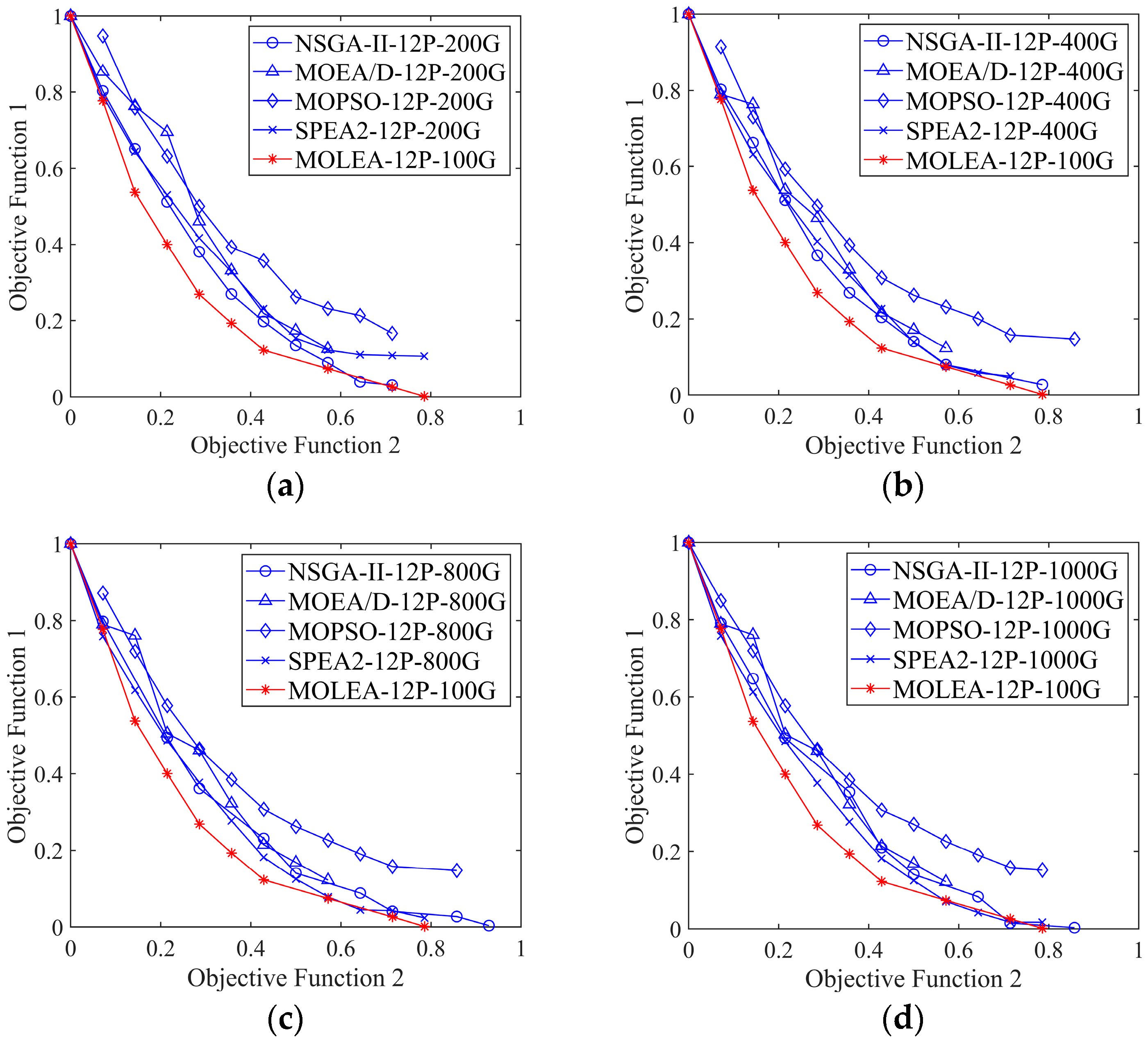
This paper has proposed a multi-objective learning evolutionary algorithm MOLEA based on DRL to solve the regional mission planning problem of imaging satellites. In the MOLEA, the DRL was used to simultaneously configure multiple evolutionary parameters according to the population state to maximize the cumulative benefit, considerably improving the convergence efficiency of the MOLEA. The proposed MOLEA effectively improves the training speed by replacing the practical application problem with the improved multi-objective functions as the training function. To the best of our knowledge, the MOLEA first proposed considering HV as the evolutionary reward of the multi-objective optimization problem. It achieves the ingenious combination of MOEA and DRL. Experimental results revealed that the proposed autonomous parameter configuration method could effectively improve the convergence speed of the algorithm in solving application problems. For the mission planning in Hubei, the planning solution obtained by MOLEA evolution for 100 generations was better than that obtained by the comparison algorithms evolution for 1000 generations. In terms of running time, the MOLEA improved by more than five times.

The proposed MOLEA is particularly suitable for application problems with high requirements for optimal solutions. The parameter configuration method studied in this paper is not limited to a multi-objective evolutionary algorithm, which can provide a reference for MOEA based on genetic algorithm, differential evolutionary, and particle swarm optimization. However, the parameter configuration of MOEAs is still an important issue that is easily overlooked, and the MOEAs based on DRL are still in the nascent stage of development. In the proposed MOLEA, the parameters’ autonomous decision configuration based on DRL is only limited to small-scale problems, and the performance of training data is degraded when testing problems have different scales. In the future, we will study more stable MOEAs based on DRL to solve larger-scale application problems. Moreover, the proposed MOLEA can be used as a theoretical basis for future multi-objective optimization algorithms and satellite imaging mission planning research.

References

1. Lu, D.; Tian, H.; Zhou, G.; Ge, H. Regional mapping of human settlements in southeastern China with multi-sensor remotely sensed data. Remote Sens. Environ. 2008, 112, 3668–3679. [Google Scholar] [CrossRef]
2. Li, D.; Wang, Y.; Shao, Z. Informatization Surveying and Mapping in the New Geographic Information Age. J. Wuhan Univ. (Inf. Sci. Ed.) 2012, 37, 1–6+134. [Google Scholar]
3. Govekar, P.D.; Griffin, C.; Beggs, H. Multi-Sensor Sea Surface Temperature Products from the Australian Bureau of Meteorology. Remote Sens. 2022, 14, 3785. [Google Scholar] [CrossRef]
4. Li, T.; Hu, D.; Wang, Y.; Di, Y.; Liu, M. Correcting remote-sensed shaded image with urban surface radiative transfer model. Int. J. Appl. Earth Obs. 2022, 106, 102654. [Google Scholar] [CrossRef]
5. Yin, H.; Weng, L.; Li, Y.; Xia, M.; Hu, K.; Lin, H.; Qian, M. Attention-guided siamese networks for change detection in high-resolution remote sensing images. Int. J. Appl. Earth Obs. 2023, 117, 103206. [Google Scholar] [CrossRef]
6. Xuan, J.; Xin, Z.; Liao, G.; Huang, P.; Wang, Z.; Sun, Y. Change Detection Based on Fusion Difference Image and Multi-Scale Morphological Reconstruction for SAR Images. Remote Sens. 2022, 14, 3604. [Google Scholar] [CrossRef]
7. Lu, Z.; Shen, X.; Li, D.; Li, D.; Chen, Y.; Wang, D.; Shen, S. Multiple super-agile satellite collaborative mission planning for area target imaging. Int. J. Appl. Earth Obs. 2023, 117, 103211. [Google Scholar] [CrossRef]
8. Sharma, S.; Kumar, V. A Comprehensive Review on Multi-objective Optimization Techniques: Past, Present and Future. Arch. Comput. Methods Eng. 2022, 29, 5605–5633. [Google Scholar] [CrossRef]
9. Tian, Y.; Cheng, R.; Zhang, X.; Jin, Y. PlatEMO: A MATLAB platform for evolutionary multi-objective optimization [educational forum]. IEEE Comput. Intell. Mag. 2017, 12, 73–87. [Google Scholar] [CrossRef] [Green Version]
10. Lin, Q.; Liu, S.; Zhu, Q.; Tang, C.; Song, R.; Chen, J.; Coello, C.A.C.; Wong, K.; Zhang, J. Particle swarm optimization with a balanceable fitness estimation for many-objective optimization problems. IEEE Trans. Evol. Comput. 2016, 22, 32–46. [Google Scholar] [CrossRef]
11. Kropp, I.; Nejadhashemi, A.P.; Deb, K. Benefits of sparse population sampling in multi-objective evolutionary computing for large-Scale sparse optimization problems. Swarm Evol. Comput. 2022, 69, 101025. [Google Scholar] [CrossRef]
12. Karafotias, G.; Hoogendoorn, M.; Eiben, A.E. Parameter Control in Evolutionary Algorithms: Trends and Challenges. IEEE Trans. Evol. Comput. 2015, 19, 167–187. [Google Scholar] [CrossRef]
13. Eiben, A.E.; Smith, J. From evolutionary computation to the evolution of things. Nature 2015, 521, 476–482. [Google Scholar] [CrossRef]
14. Deng, W.; Zhang, X.; Zhou, Y.; Liu, Y.; Zhou, X.; Chen, H.; Zhao, H. An enhanced fast non-dominated solution sorting genetic algorithm for multi-objective problems. Inform. Sci. 2022, 585, 441–453. [Google Scholar] [CrossRef]
15. Huang, C.; Li, Y.; Yao, X. A survey of automatic parameter tuning methods for metaheuristics. IEEE Trans. Evol. Comput. 2019, 24, 201–216. [Google Scholar] [CrossRef]
16. Parpinelli, R.S.; Plichoski, G.F.; Silva, R.S.D.; Narloch, P.H. A review of techniques for online control of parameters in swarm intelligence and evolutionary computation algorithms. Int. J. Bio-Inspir. Comput. 2019, 13, 1–20. [Google Scholar] [CrossRef]
17. Li, S.; Shen, X.; Yao, H.; Zhang, G.; Liu, Y. An optimization method for the roll angle of circumlunar satellites for regional imaging missions. J. Wuhan Univ. (Inf. Sci. Ed.) 2019, 44, 593–600. [Google Scholar]
18. Ming, F.; Gong, W.; Yang, Y.; Liao, Z. Constrained multimodal multi-objective optimization: Test problem construction and algorithm design. Swarm Evol. Comput. 2023, 76, 101209. [Google Scholar] [CrossRef]
19. Dai, L.; Zhang, L.; Chen, Z.; Ding, W. Collaborative granular sieving: A deterministic multi-evolutionary algorithm for multimodal optimization problems. Inform. Sci. 2022, 613, 288–308. [Google Scholar] [CrossRef]
20. Xue, Y.; Tang, T.; Pang, W.; Liu, A.X. Self-adaptive parameter and strategy based particle swarm optimization for large-scale feature selection problems with multiple classifiers. Appl. Soft Comput. 2020, 88, 106031. [Google Scholar] [CrossRef]
21. Yang, H.; Tao, S.; Zhang, Z.; Cai, Z.; Gao, S. Spatial information sampling: Another feedback mechanism of realizing adaptive parameter control in meta-heuristic algorithms. Int. J. Bio-Inspir. Comput. 2022, 19, 48–58. [Google Scholar] [CrossRef]
22. Bao, Q.; Wang, M.; Dai, G.; Chen, X.; Song, Z. Dynamical decomposition and selection based evolutionary algorithm for many-objective optimization. Appl. Soft Comput. 2023, 141, 110295. [Google Scholar] [CrossRef]
23. Xue, Y.; Cai, X.; Neri, F. A multi-objective evolutionary algorithm with interval based initialization and self-adaptive crossover operator for large-scale feature selection in classification. Appl. Soft Comput. 2022, 127, 109420. [Google Scholar] [CrossRef]
24. Eiben, A.E.; Schut, M.C.; de Wilde, A.R. Is Self-adaptation of Selection Pressure and Population Size Possible?—A Case Study. In Parallel Problem Solving from Nature—PPSN IX, Proceedings of the International Conference on Parallel Problem Solving from Nature; Runarsson, T.P., Beyer, H., Burke, E., Merelo-Guervós, J.J., Whitley, L.D., Yao, X., Eds.; Springer: Berlin/Heidelberg, Germany, 9 September 2006; pp. 900–909. [Google Scholar]
25. Botvinick, M.; Ritter, S.; Wang, J.X.; Kurth-Nelson, Z.; Blundell, C.; Hassabis, D. Reinforcement Learning, Fast and Slow. Trends Cogn. Sci. 2019, 23, 408–422. [Google Scholar] [CrossRef] [PubMed] [Green Version]
26. Eiben, A.E.; Michalewicz, Z.; Schoenauer, M.; Smith, J.E. Parameter control in evolutionary algorithms. In Parameter Setting in Evolutionary Algorithms; Springer: Berlin/Heidelberg, Germany, 2007; pp. 19–46. [Google Scholar]
27. Mnih, V.; Kavukcuoglu, K.; Silver, D.; Rusu, A.A.; Veness, J.; Bellemare, M.G.; Graves, A.; Riedmiller, M.; Fidjeland, A.K.; Ostrovski, G.; et al. Human-level control through deep reinforcement learning. Nature 2015, 518, 529–533. [Google Scholar] [CrossRef]
28. Schuchardt, J.; Golkov, V.; Cremers, D. Learning to evolve. arXiv 2019, arXiv:1905.03389. [Google Scholar]
29. Li, K.; Zhang, T.; Wang, R. Deep Reinforcement Learning for Multiobjective Optimization. IEEE Trans. Cybern. 2021, 51, 3103–3114. [Google Scholar] [CrossRef] [PubMed] [Green Version]
30. Song, Y.; Wei, L.; Yang, Q.; Wu, J.; Xing, L.; Chen, Y. RL-GA: A Reinforcement Learning-based Genetic Algorithm for Electromagnetic Detection Satellite Scheduling Problem. Swarm Evol. Comput. 2023, 77, 101236. [Google Scholar] [CrossRef]
31. Tian, Y.; Li, X.; Ma, H.; Zhang, X.; Tan, K.C.; Jin, Y. Deep Reinforcement Learning Based Adaptive Operator Selection for Evolutionary Multi-Objective Optimization. IEEE Trans. Emerg. Top. Comput. Intell. 2022, 7, 1051–1064. [Google Scholar] [CrossRef]
32. Reijnen, R.; Zhang, Y.; Bukhsh, Z.; Guzek, M. Deep Reinforcement Learning for Adaptive Parameter Control in Differential Evolution for Multi-Objective Optimization. In Proceedings of the 2022 IEEE Symposium Series on Computational Intelligence (SSCI), Singapore, 4–7 December 2022; pp. 804–811. [Google Scholar]
33. Li, T.; Meng, Y.; Tang, L. Scheduling of Continuous Annealing With a Multi-Objective Differential Evolution Algorithm Based on Deep Reinforcement Learning. IEEE Trans. Autom. Sci. Eng. 2023; Early Access. [Google Scholar]
34. Chen, Y.; Xu, M.; Shen, X.; Zhang, G.; Lu, Z.; Xu, J. A Multi-Objective Modeling Method of Multi-Satellite Imaging Task Planning for Large Regional Mapping. Remote Sens. 2020, 12, 344. [Google Scholar] [CrossRef] [Green Version]
35. Schulman, J.; Wolski, F.; Dhariwal, P.; Radford, A.; Klimov, O. Proximal Policy Optimization Algorithms. arXiv 2017, arXiv:1707.06347. [Google Scholar]
36. Hedar, A.R. Global Optimization Test Problems. 2016. Available online: http://www-optima.amp.i.kyoto-u.ac.jp/member/student/hedar/Hedar_files/TestGO.htm (accessed on 15 January 2020).
37. Surjanovic, S.; Bingham, D. Virtual Library of Simulation Experiments: Test Functions and Datasets. 2017. Available online: https://www.sfu.ca/ssurjano/optimization.html (accessed on 15 January 2020).
38. Schulman, J.; Moritz, P.; Levine, S.; Jordan, M.; Abbeel, P. High-dimensional continuous control using generalized advantage estimation. arXiv 2015, arXiv:1506.02438. [Google Scholar]
39. Deb, K.; Pratap, A.; Agarwal, S.; Meyarivan, T. A fast and elitist multi-objective genetic algorithm: NSGA-II. IEEE Trans. Evol. Comput. 2002, 6, 182–197. [Google Scholar] [CrossRef] [Green Version]
40. Zhang, Q.; Li, H. MOEA/D: A multiobjective evolutionary algorithm based on decomposition. IEEE Trans. Evol. Comput. 2007, 11, 712–731. [Google Scholar] [CrossRef]
41. Mofid, H.; Jazayeri-Rad, H.; Shahbazian, M.; Fetanat, A. Enhancing the performance of a parallel nitrogen expansion liquefaction process (NELP) using the multi-objective particle swarm optimization (MOPSO) algorithm. Energy 2019, 172, 286–303. [Google Scholar] [CrossRef]
42. Wahid, A.; Gao, X.; Andreae, P. Multi-objective clustering ensemble for high-dimensional data based on Strength Pareto Evolutionary Algorithm (SPEA-II). In Proceedings of the 2015 IEEE International Conference on Data Science and Advanced Analytics (DSAA), Paris, France, 19–21 October 2015; pp. 1–9. [Google Scholar]
43. Muzid, S. An Adaptive Approach to Controlling Parameters of Evolutionary Algorithms. J. Phys. Conf. Ser. 2020, 1430, 12048. [Google Scholar] [CrossRef]
44. Haiquan, S.U.N.; Wei, X.I.A.; Xiaoxuan, H.U.; Chongyan, X.U. Earth observation satellite scheduling for emergency tasks. J. Syst. Eng. Electron. 2019, 30, 931–945. [Google Scholar]
45. Cui, K.; Xiang, J.; Zhang, Y. Mission planning optimization of video satellite for ground multi-object staring imaging. Adv. Space Res. 2018, 61, 1476–1489. [Google Scholar] [CrossRef]
46. Kim, J.; Ahn, J.; Choi, H.; Cho, D. Task Scheduling of Agile Satellites with Transition Time and Stereoscopic Imaging Constraints. J. Aerosp. Inf. Syst. 2020, 17, 285–293. [Google Scholar] [CrossRef]
47. Lu, Z.; Shen, X.; Li, D.; Chen, Y. Integrated Imaging Mission Planning Modeling Method for Multi-Type Targets for Super-Agile Earth Observation Satellite. IEEE J. Sel. Top. Appl. Earth Obs. Remote Sens. 2022, 15, 4156–4169. [Google Scholar] [CrossRef]
48. Qiu, W.; Xu, C.; Ren, Z.; Teo, K.L. Scheduling and Planning Framework for Time Delay Integration Imaging by Agile Satellite. IEEE Trans. Aerosp. Electron. Syst. 2022, 58, 189–205. [Google Scholar] [CrossRef]
49. Young, S.R.; Rose, D.C.; Karnowski, T.P.; Lim, S.; Patton, R.M. Optimizing deep learning hyper-parameters through an evolutionary algorithm. In Proceedings of the Workshop on Machine Learning in High-Performance Computing Environments; Association for Computing Machinery, Austin, TX, USA, 15 November 2015. [Google Scholar]
50. Martín, A.; Lara-Cabrera, R.; Fuentes-Hurtado, F.; Naranjo, V.; Camacho, D. EvoDeep: A new evolutionary approach for automatic Deep Neural Networks parametrization. J. Parallel Distr. Com. 2018, 117, 180–191. [Google Scholar] [CrossRef]
51. Ma, W.; Wan, L.; Yu, C.; Zou, L.; Zheng, J. Multi-objective optimization of traffic signals based on vehicle trajectory data at isolated intersections. Transp. Res. Part C Emerg. Technol. 2020, 120, 102821. [Google Scholar] [CrossRef]
52. Ji, B.; Zhang, D.; Yu, S.S.; Zhang, B. Optimally solving the generalized serial-lock scheduling problem from a graph-theory-based multi-commodity network perspective. Eur. J. Oper. Res. 2021, 288, 47–62. [Google Scholar] [CrossRef]
53. Yang, X.; Yang, Y.; Li, Y.; Yang, X. Path planning for guided passengers during evacuation in subway station based on multi-objective optimization. Appl. Math. Model. 2022, 111, 777–801. [Google Scholar] [CrossRef]
Figure 1. MOLEA framework.
Remotesensing 15 03932 g001
Figure 2. Population state coding.
Remotesensing 15 03932 g002
Figure 3. Neural network architecture. (a) The overall neural network architecture; (b) ‘Pool, replicate, conv’ sub-structure of the neural network.
Remotesensing 15 03932 g003
Figure 4. Schematic of HV calculation.
Remotesensing 15 03932 g004
Figure 5. Distribution of non-dominated solutions of various algorithms for mission planning in Hubei.
Remotesensing 15 03932 g005
Figure 6. Distribution of non-dominated solutions for different agents in Hubei.
Remotesensing 15 03932 g006
Figure 7. Changes in HV of various algorithms with evolutionary generations.
Remotesensing 15 03932 g007
Figure 8. Distribution of non-dominated solutions of various algorithms with the same population size 12 but different evolutionary generations. MOLEA evolution for 100 generations. (a) Comparison algorithms evolution for 200 generations. (b) Comparison algorithms evolution for 400 generations. (c) Comparison algorithms evolution for 800 generations. (d) Comparison algorithms evolution for 1000 generations.
Remotesensing 15 03932 g008
Figure 9. Distribution of non-dominated solutions for various algorithms in the same evolutionary generation 100 but with different population sizes. The population size of the MOLEA is 12. (a) The population size of the comparison algorithms is 20. (b) The population size of the comparison algorithms is 40.
Remotesensing 15 03932 g009
Figure 10. Distribution of non-dominated solutions at various population sizes and evolutionary generations in Congo (K). (a) population size 12 and 100 generations. (b) population size 12 and 200 generations. (c) population size 20 and 100 generations. (d) population size 40 and 100 generations.
Remotesensing 15 03932 g010
Figure 11. Hubei coverage results. (a) MOLEA-12P-100G (b) NSGA-II-12P-1000G (c) MOEA/D-12P-1000G (d) MOPSO-12P-1000G (e) SPEA2-12P-1000G.
Remotesensing 15 03932 g011
Figure 12. Congo (K) Coverage results. (a) MOLEA-40P-100G. (b) NSGA-II-40P-100G. (c) MOEA/D-40P-100G. (d) MOPSO-40P-100G. (e) SPEA2-40P-100G.
Remotesensing 15 03932 g012