Simulation of the Ecological Service Value and Ecological Compensation in Arid Area: A Case Study of Ecologically Vulnerable Oasis

Abstract

In recent years, the delicate balance between economic development and ecological environment protection in ecologically fragile arid areas has gradually become apparent. Although previous research has mainly focused on changes in ecological service value caused by land use, a comprehensive understanding of ecology–economy harmony and ecological compensation remains elusive. To address this, we employed a coupled deep learning model (convolutional neural network-gated recurrent unit) to simulate the ecological service value of the Wuwei arid oasis over the next 10 years. The ecology–economy harmony index was used to determine the priority range of ecological compensation, while the GeoDetector analyzed the potential impact of driving factors on ecological service value from 2000 to 2030. The results show the following: (1) The coupled model, which extracts spatial features in the neighborhood of historical data using a convolutional neural network and adaptively learns time features using the gated recurrent unit, achieved an overall accuracy of 0.9377, outperforming three other models (gated recurrent unit, convolutional neural network, and convolutional neural network—long short-term memory); (2) Ecological service value in the arid oasis area illustrated an overall increasing trend from 2000 to 2030, but urban expansion still caused a decrease in ecological service value; (3) Historical ecology–economy harmony was mainly characterized by low conflict and potential crisis, while future ecology–economy harmony will be characterized by potential crisis and high coordination. Minqin and Tianzhu in the north and south have relatively high coordination between ecological environment and economic development, while Liangzhou and Guluang in the west and east exhibited relatively low coordination, indicating a greater urgency for ecological compensation; (4) Geomorphic, soil, and digital elevation model emerged as the most influential natural factor affecting the spatial differentiation of ecological service value in the arid oasis area. This study is of great significance for balancing economic development and ecological protection and promoting sustainable development in arid areas.

1. Introduction

The benefits that people derive from multiple processes and ecosystem functions can be described as ecosystem services [1]. Driven by the growth of urban demand, land use change has led to serious degradation of global ecosystems [2,3]. On the one hand, the invasion of large areas of ecological land has resulted in irreversible biodiversity loss [4]. On the other hand, local climate change, the urban heat island effect, and changes in precipitation have contributed to the decline in the Ecological service value (ESV) [5]. With population growth and economic development, global ecosystems have been seriously damaged, and the imbalance between economic development and ecological environment protection has gradually become prominent, especially in ecologically fragile arid areas [6,7]. In arid regions, characterized by harsh climatic conditions, soil salinization and alkalization, and the sustainability of ecosystem services has always been a focus of attention [8,9]. Oasis ecosystems play an essential role in social and economic stability and development in arid areas, but their ecological fragility is particularly pronounced due to the low precipitation and high evaporation rates [10,11]. Wuwei Oasis is situated in the Shiyang River Basin, an important inland river in Northwest China’s ecologically fragile area, and its ecological environment quality has a serious impact on the entire basin [12,13]. Therefore, focusing on the ESV and EEH in the arid oasis area of Wuwei is of great significance for promoting sustainable development and achieving a balance between economic growth and ecological protection [14].

Ecological services are characterized by complex interconnections and strong scale effects, with changes in ESV often being determined by multiple ecosystem services [15]. The benefit transfer method can not only rapidly assess the individual ecological benefits of multiple ecosystem services but also evaluate their overall ecological benefits, and therefore, it has been widely used in ESV evaluation [16]. However, the benefit transfer method relies on equivalent factor coefficients to characterize the relationship between different land use types and ESV, which is subjective. In addition, there is spatiotemporal heterogeneity in land use distribution. Thus, it is necessary to adjust the coefficient value of multiple ecosystem services according to the natural and socioeconomic characteristics of the area to improve the accuracy of ESV estimates.

Assessing the impact of future land use changes on ESV and Ecology–Economy Harmony (EEH) can provide scientific policy recommendations for ecosystem management [17]. Li, et al. [18] employed the InVEST and SLEUTH models to evaluate the impact of land use changes on habitat quality. However, existing models often have difficulty in reliably predicting future land use changes, leading to significant errors in evaluation results [19]. Deep learning has recently emerged as a powerful tool for time-series object modeling, demonstrating excellent performance in various domains [20]. It can not only extract implicit spatial features from datasets with multiple variables to improve feature representation ability [21] but also exploit long-term time dependencies among large amounts of time-series data to establish accurate feature maps [22]. Among the various deep learning models, convolutional neural networks (CNN) have been extensively utilized in the dynamic simulation of time-series data. Zhai, et al. [23] fused CNN and vector-based cellular automata to extract high-level features of irregularly shaped cells in the neighborhood and simulate land use changes, achieving higher simulation accuracy than other models such as Random Forest and Artificial Neural Networks. Qian, et al. [24] also validated the effectiveness of deep learning models such as CNN applying land use data from Shanghai from 2000 to 2015. However, existing studies exploring neighborhood effects in transformation rules have only considered the extraction of spatial features in historical data dimensions, ignoring the significant long-term time dependencies in neighborhood interactions, resulting in low simulation accuracy [25]. A gated recurrent unit (GRU) network is a deep learning model used to extract time-dimension features. Compared with traditional recurrent neural networks, it can improve memory capacity and training performance and better solve overfitting, gradient vanishing, and explosion problems. Cao, et al. [26] predicted grain loss and waste rates based on a multi-task multi-gate recurrent unit autoencoder method, and the results indicated that the accuracy of this method was higher than that of existing models. Chen, et al. [27] applied the GRU network to predict long-term degradation trends based on available data on degradation features. In light of the excellent performance of the GRU in time feature extraction, we coupled the CNN-GRU model to complement the deficiencies in existing time-series data simulation research.

Ecological compensation is a widely recognized economic approach to improving water yield, soil and water conservation, intensive and efficient use of water resources, ecological, environmental protection, and pollution control by coordinating the relationships between different stakeholders [28]. There exist various methods for evaluating ecological compensation, including the willingness-to-pay, opportunity cost, ecological footprint, and value theory methods [29,30]. While the willingness-to-pay method relies on subjective survey data [31], the opportunity cost method tends to undervalue ecosystem services by focusing on cost-benefit analysis [32]. Similarly, the ecological footprint method determines the sustainability of ecological compensation by evaluating the supply and demand relationship between humans and ecological resources, but its sustainability is weak [33]. The ecological service value method, which is based on the theory of externalities, bridges the gap between natural ecosystems and economic systems by quantifying the direct or indirect available ecological value used to produce ecosystem services [34]. It quantifies ecological compensation by comparing the non-market ESV per unit area with the GDP per unit area of the area. Although ESV is complex and unstable at cross-regional scales, it can be corrected by incorporating various regional data, such as food and GDP, and is applicable to a wide range of research scales [35]. Consequently, ESV evaluation appears to be a more suitable method for ecological compensation. In addition, EEH is a critical foundation for setting reasonable ecological compensation standards and accurately quantifying ecological compensation, which has often been frequently overlooked in previous research. ESV comprises various ecosystem services, including supply, regulation, support, and cultural services, and exploring the ESV represented by different ecosystem services is necessary to fully express the EEH of the area, serving ecological compensation and sustainable development.

A thorough analysis of the influencing factors and mechanisms of ESV is a crucial basis for guiding ecological protection decision-making [36]. Wu et al. [17] quantitatively analyzed the impact of rapid urbanization on ecosystem services in Kunshan from 2006 to 2030. Chen, et al. [37] utilized cellular automata and geographically weighted regression to simulate the ESV loss caused by land use changes in Chongqing. Previous studies have primarily focused on the rise or fall of ESV caused by land use changes, but little is known about the driving mechanisms of ESV, particularly in arid areas [38,39]. Research methods for ESV and its driving factors have primarily included principal component and correlation analysis [40], regression models, and grey relational analysis [41]. Although these methods can explain the contribution of influencing factors to a certain extent, they fail to capture the interaction and joint effects between influencing factors and cannot fully express the complex spatial correlation and spatiotemporal differentiation characteristics within ESV [42]. GeoDetector can further reveal the spatial distribution relationship and interaction mechanism between independent and dependent variables from a statistical perspective by converting qualitative data into quantitative data [43,44]. Therefore, this study utilizes GeoDetector to quantitatively analyze the explanatory power of each driving factor for spatial variable distribution characteristics and explore the interaction between two factors [45].

The main contributions of this study are as follows:

(1) Proposed a new CNN-GRU model, which integrates both temporal and spatial neighborhood features, for simulating the dynamic process of land use change. This approach outperforms three other models, including GRU, CNN, and CNN long short-term memory (LSTM), and provides higher accuracy in predicting land use change;

(2) Revealed the impact of land use change on ESV in the arid oasis area of Northwest China;

(3) Determined EEH in the historical period and the next 10 years in the arid oasis area, as well as the priority for ecological compensation;

(4) Employed the GeoDetector to explore the driving mechanism of ESV;

2. Study Area and Data Sources

2.1. Study Area

Wuwei (Figure 1) (36°29′~39°27′N, 101°49′~104°16′E) is located in Northwest China, at the intersection of the Loess Plateau, the Qinghai–Tibet Plateau, and the Mongolian Plateau [46]. The terrain is complex, with the southern area belonging to the Qilian Mountains, and the climate is suitable for the development of forestry and animal husbandry. The central area is a flat oasis area with fertile land and is an important agricultural production base in China. The northern area is a desert area with low precipitation [12]. Wuwei spans 326 km in length and 204 km in width and has natural landscapes, such as snow-covered highlands, oases, and deserts. The permanent population was 1.825 × 10⁴ at the end of 2019 [13].

2.2. Data Sources

The land use datasets for 2000, 2010, and 2020 were obtained from the Global Geographic Information Products Platform for this study. The driving factors were categorized into four types: transportation accessibility; socioeconomic conditions; terrain conditions; and climate conditions, consisting of 14 categories. Data sources for each category are presented in

Table A1. Data Format and Source.

Category	Data	Data Format	Data Sources	Spatial Resolution
Traffic accessibility	distance to the settlement	vector (Point)	National Geographic Information Resource Directory Service System (https://webmap.cn/) accessed on 1 January 2022	30 m
	distance to road	vector (Polyline)	National Geographic Information Resource Directory Service System (https://webmap.cn/) accessed on 1 January 2022	30 m
	distance to railway	vector (Polyline)	National Geographic Information Resource Directory Service System (https://webmap.cn/) accessed on 1 January 2022	30 m
	distance to river	vector (Polyline)	National Geographic Information Resource Directory Service System (https://webmap.cn/) accessed on 1 January 2022	30 m
	distance to ecological function protection area	vector (Polygont)	Resource and Environmental Science and Data Center, Chinese Academy of Sciences (http://www.resdc.cn/) accessed on 1 January 2022	30 m
Social and economic conditions	population	raster	Resource and Environmental Science and Data Center, Chinese Academy of Sciences (http://www.resdc.cn/) accessed on 2 January 2022	30 m
	GDP	raster	Resource and Environmental Science and Data Center, Chinese Academy of Sciences (http://www.resdc.cn/) accessed on 2 January 2022	30 m
	nighttime lights	rasterd	Hubei high-resolution earth observation system application platform (http://59.175.109.173:8888) accessed on 2 January 2022	30 m
	NPP	raster	Resource and Environmental Science and Data Center, Chinese Academy of Sciences (http://www.resdc.cn/) accessed on 2 January 2022	30 m
Terrain conditions	elevation	raster	USGS Earth Explorer (https://earthexplorer.usgs.gov/) accessed on 3 January 2022	30 m
	slope	raster	USGS Earth Explorer (https://earthexplorer.usgs.gov/) accessed on 3 January 2022	30 m
	fault	vector (Polyline)	“Hydrogeological Map of Gansu Province” (Gansu Geological and Mineral Bureau Hydrogeological Engineering Geological Survey Institute) (http://www.gssgy.com/) accessed on 3 January 2022	30 m
Climatic conditions	temperature	raster	Resource and Environmental Science and Data Center, Chinese Academy of Sciences (http://www.resdc.cn/) accessed on 4 January 2022	30 m
	precipitation	raster	Resource and Environmental Science and Data Center, Chinese Academy of Sciences (http://www.resdc.cn/) accessed on 4 January 2022	30 m

of the attached Appendix. Transportation accessibility variables included major roads, railways, rivers, residential areas, and ecological function protection areas, while socioeconomic variables included nighttime lights, GDP, population, and NPP. Terrain conditions included elevation, slope, and faults, while conditions included precipitation and temperature. All data were resampled to a spatial resolution of 30 m and normalized to ensure consistency across variables. In the initial phase, remote sensing images were acquired, and an extensive data preprocessing pipeline was implemented. This preprocessing encompassed radiometric calibration, atmospheric correction, geometric correction, image mosaicking, and cropping. These rigorous steps were undertaken to rectify image distortions, geometric irregularities, and atmospheric interferences arising from sensor characteristics, spatial variations, atmospheric absorption, scattering, and other influential factors. Subsequently, we leveraged a land use remote sensing dataset to obtain comprehensive land use classification data. Additionally, key remote sensing variables, such as nighttime lights, were strategically integrated as driving factors into the CNN-GRU algorithm. This integration facilitated the acquisition of spatiotemporal features, thereby enabling the model to effectively learn and process complex temporal dynamics and land use patterns.

3. Methods

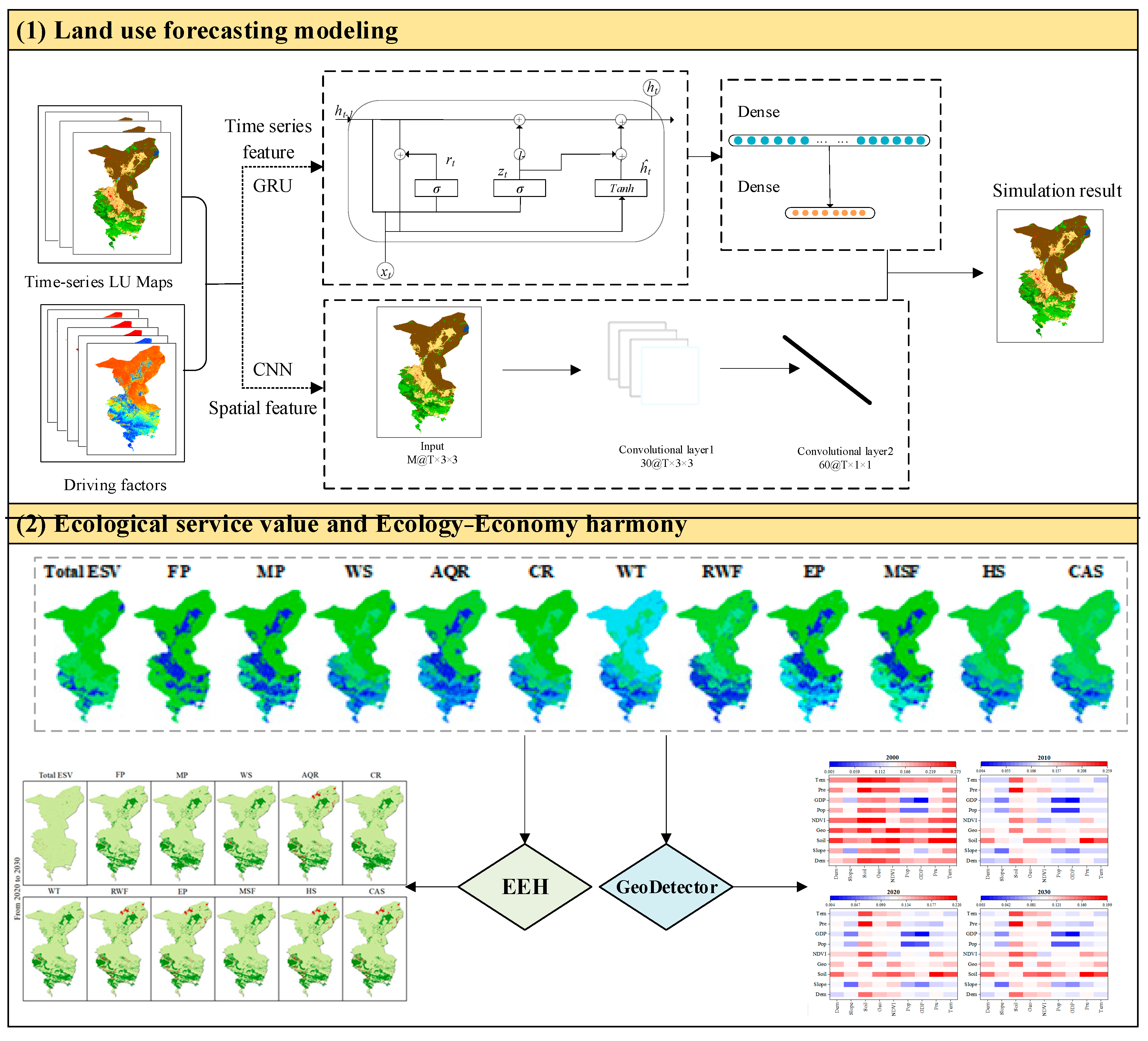
The research framework is illustrated in Figure 2.

3.1. Land Use Modeling

3.1.1. CNN

The CNN architecture typically comprises convolutional layers, pooling layers, activation functions, and fully connected layers [47]. Convolutional layers extract the spatial features of the input image by using filters learned from the training data set. Usually, an activation function is used after the convolutional layers to introduce nonlinearity into the network and capture the complex relationship between the input and output [48]. After the activation function, a pooling layer is added to retain the main features of the convolutional layer while reducing parameters. Finally, the objective of the fully connected layer is to predict the output value based on a nonlinear combination of a series of feature maps from convolutional and pooling layers. The core of this study is to use CNN to extract the complex spatial features of the data and pooling layers are omitted to prevent the loss of relevant features [49].

3.1.2. GRU

GRU calculates the probability distribution of the time series data by employing the encoder and decoder [50]. Initially, the conditional distribution on a variable-length output sequence given another variable-length sequence is learned (e.g., $p(y_1,...,y_{T\prime }|x_{1,\hspace{0.33em}...\hspace{0.33em},}{x}_T)$, where T and $T\prime$ are the input and output sequences, respectively. Secondly, the encoder reads the temporal features of the input sequence x in order. The hidden state h_(t) changes with the time step (Equation (1)). Upon reading the sequence end, h_(t) is the summary of the entire input sequence c. The decoder is trained to generate the output sequence by predicting the time dimension feature y_t of the next neighboring unit. The hidden state at time t is determined by Equation (2). Using the softmax activation function to predict the probability distribution of the next neighboring unit learning sequence (Equation (3)), the output of each time step t is the conditional distribution $p\left(x_t\right|x_{t-1,\hspace{0.33em}...\hspace{0.33em},}{x}_1)$. By combining the probability of each neighboring unit, the probability of sequence x is calculated by Equation (4). Therefore, the conditional distribution of the time dimension feature of the next neighboring unit is Equation (5) [51].

$$h_{\left(t\right)}=f(h_{(t-1)},x_t)$$

(1)

$$h_{\left(t\right)}=f(h_{(t-1)},y_{(t-1)},c)$$

(2)

$$p(x_{(t,j)}=1|x_{t-1},...,x_1)=\frac{\mathit{exp}(w_j{h}_{\left(t\right)})}{{\sum }_{j\prime =1}^K\mathit{exp}(w_{j\prime }{h}_{\left(t\right)})}$$

(3)

$$p(x)=\prod _{t=1}^T{p}_t\left(x\right|x_{t-1},...,x_1)$$

(4)

$$p\left(y_t\right|y_{(t-1)},y_{(t-2)},...,y_1,c)=g(h_{\left(t\right)},y_{(t-1)},c)$$

(5)

Here, f is a non-linear activation function; w_j is the row of weight matrix w. For a given activation function g, it must generate effective probabilities.

The activation calculation for the jth hidden unit is given by:

$$r_j=\sigma \left(\right[W_{r}x{]}_j+\left[U_r{h}_{(t-1)}{]}_j\right)$$

(6)

$$z_j=\sigma \left(\right[W_{z}x{]}_j+\left[U_z{h}_{(t-1)}{]}_j\right)$$

(7)

$$h_j^{\left(t\right)}=z_j{h}_j^{(t-1)}+(1-z_j){\tilde{h}}_j^{\left(t\right)}$$

(8)

$${\tilde{h}}_j^{\left(t\right)}=f([Wx{]}_j+r_j[U{h}_{(t-1)}])$$

(9)

Here, r_j represents the reset gate; z_j represents the update gate; h_j represents the actual activation of the unit; σ is the sigmoid function; [.]_j represents the jth element of the vector; x and h_(t−1) are the input state and the previous hidden state, and W_r and U_r are weight matrices.

When the reset gate is close to 0, the hidden state is forced to ignore the previous hidden state and only use the current input to reset. The update gate controls the amount of information transferred from the previous hidden state to the current hidden state for the long-term memory [52]. Each hidden unit has separate reset and update gates, so it can learn to capture dependencies at different time scales.

3.1.3. CNN-GRU

To optimize the land-use change simulation research, we constructed a six-layer network structure consisting of two CNN layers, two GRU layers, and two fully connected layers. The two convolutional layers each consist of 14 3 × 3 convolutional kernels, resulting in a (N − 2) × (N − 2) × 14 feature map. The data were then formatted with 14 time steps and one input feature per time step. The first GRU layer has 64 cores, with h_(t) being passed to the next layer at each time step. The second GRU layer has 94 cores and only outputs h_(t) at the final time step. To avoid overfitting, the dropout rate was set to 20% for both GRU layers, and the tanh activation function was chosen to improve model performance. Finally, there are two fully connected layers, with 128 neurons in the first layer and a dropout rate of 20% and 8 neurons in the second layer with a softmax classifier. After continuous iteration, we found that the optimal learning rate for the research area data was 0.002; the batch size was set to 128, and the Adam algorithm was selected as the optimizer. Further, the cross-entropy loss function was introduced to optimize model performance. The number of epochs was set to 50, the loss value decreased rapidly to a certain point, and the iteration process basically converged.

The modeling process consists of four steps: (1) Data preprocessing and model training: preprocessing land use historical data and driving factor variables to prepare for training and conversion rules; (2) Model calibration: utilizing CNN and GRU algorithms to extract spatial and temporal neighborhood features of land use and driving factors, continuously optimizing the model’s performance; (3) Model validation: comparing the simulated land use change results in the CNN, GRU, CNN-LSTM, and CNN-GRU models with the actual situation using the same data set; (4) Future prediction: using the calibrated model to simulate future land use, ESV, and EEH changes.

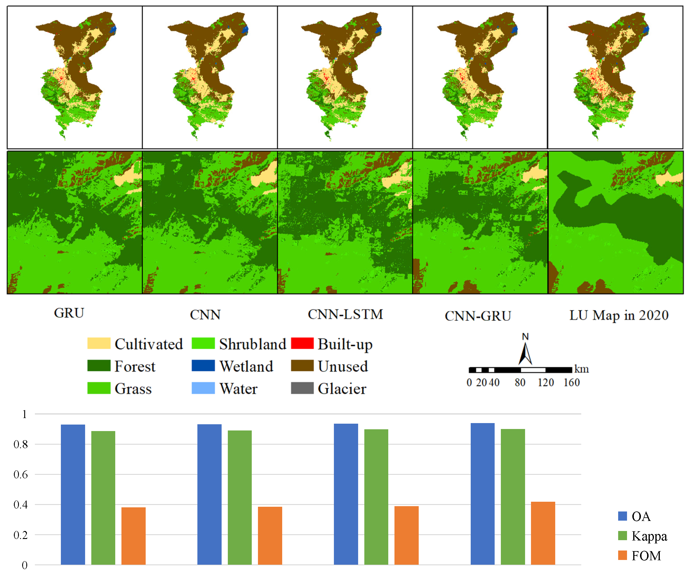
Using Python coding, we calibrated the model parameters with historical data from 2000 to 2010 and generated simulation results for 2020 (Figure 3). To verify the model performance, we compared the results with three sets of indicators, overall accuracy, Kappa coefficient, and figure of merit (FOM). Specifically, we conducted comparisons among (1) The coupled model and single models (CNN-GRU, CNN, and GRU) to examine the importance of spatiotemporal feature extraction, (2) Different recurrent neural networks (CNN-GRU and CNN-LSTM) as feature samplers for comparing the performance of time dimension feature extraction, and (3) Single spatiotemporal models (CNN and GRU) to analyze the impact of temporal and spatial features on time series data simulation.

3.2. ESV Evaluation

In this study, the ESV of Wuwei Oasis was calculated by exploiting the standard unit results and evaluation method of the ecological service value equivalent factor improved by Xie, et al. [53]. To ensure the applicability of the numerical coefficients in the calculation of ESV at the regional scale, the coefficients were adjusted based on the correction factor for grain production. The equations applied for calculating ESV are as follows:

$$E_a=\frac{1}{7}\times P\times Y$$

(10)

$$E_i=E_a\times q$$

(11)

$$ESV=\sum \left(A_i\times E_i\right)$$

(12)

Here, E_a is the economic value of an ESV equivalent factor; E_i is the ESV of the land ecosystem i per unit area; q is the ESV equivalent factor per unit area; A_i is the area of land ecosystem type I; Y is the crop yield per unit area in Wuwei, and P is the average grain price in 2020.

3.3. Ecology–Economy Harmony

ESV change serves as a pivotal gauge for assessing regional socioeconomic and ecological environment sustainability. Coordinated development between the ecological environment and the economy entails a harmonious interaction and alignment of elements within the environmental and economic subsystems throughout the regional development trajectory, fostering their reciprocal advancement and ultimately elevating the overall developmental status of the region. Through an in-depth analysis of the association between alterations in ESV resulting from land use dynamics and the level of regional socio-economic development, an assessment of the degree of harmony between the regional ecological environment and economic progress can be achieved. The ecological environment and economic development status in arid oasis areas was measured by utilizing the Ecology–Economy Harmony (EEH) index (

Table 1. Classification level of EEH index. At the coordination level, an EEH value greater than or equal to 1 denotes that the growth rate of ESV equals or surpasses the growth rate of GDP. This finding reflects a high degree of synchronization between the ecological environment and economic development within this study’s area. Alternatively, it may suggest that the ecological environment experienced significant damage initially but subsequently underwent ecological restoration, resulting in certain limitations on economic development. On the other hand, when the EEH falls within the range of 0 to 1, it indicates that the growth rate of ESV is lower than that of GDP. Despite economic development not directly causing ecological degradation, varying degrees of ecological pressure persist. A higher EEH value indicates enhanced coordination between ecological and economic factors. In the conflict level, negative ESV growth signifies that economic development has detrimental effects on ecological environment conservation, leading to disharmony between the two. A lower EEH value indicates more pronounced conflicts between economic development and ecological protection.

EEH Index	Classification Level	EEH Index	Classification Level
EEH ≥ 1	high coordination	−0.5 ≤ EEH < 0	low conflict
0.5 ≤ EEH < 1	moderate coordination	−1 ≤ EEH < −0.5	moderate conflict
0 ≤ EEH < 0.5	potential crisis	EEH ≤ −1	serious conflict

), which combines datasets of ESV and GDP of the period from 2000 to 2030. The ecological compensation priority was then determined. Additionally, the 2023 GDP data were obtained through time-series forecasting employing Python 3.9 software.

$$\mathrm{E}\mathrm{E}\mathrm{H}=\frac{\raisebox{1ex}{$\left({ESV}_{hj}-{ESV}_{hi}\right)$}\!\left/ \!\raisebox{-1ex}{${ESV}_{hi}$}\right.}{\raisebox{1ex}{$\left({GDP}_{hj}-{GDP}_{hi}\right)$}\!\left/ \!\raisebox{-1ex}{${GDP}_{hi}$}\right.}$$

(13)

Here, EEH is the ecology–economy harmony index; ESV_hj and ESV_hi are the ecosystem service values for different periods, and GDP_hj and GDP_hi are the GDP values for different periods. Coordination and conflict levels are divided based on the regional characteristics of the arid oasis area and the existing literature [54].

3.4. GeoDetector

We employed the Geodetector model to quantify the influence of various factors on the changes in ESV in the Wuwei Oasis area [43]. Geodetector is a spatial statistical method used for identifying driving factors of geographic phenomena, widely applied in the fields of geography, environmental science, and public health, among others. It has the capability to reveal the impact extent and interaction relationships of various factors on specific events or phenomena. The determination of single-factor and two-factor contributions to ESV values ranged from 0 to 1, with higher values denoting a more pronounced influence. Unlike conventional approaches employed in identifying driving factors, Geodetector demonstrates a distinctive advantage in its capacity to investigate the combined impact of two independent variables on the dependent variable. Notably, Geodetector exhibits a high degree of flexibility concerning the incorporation of input data, as it can effectively accommodate both quantitative and qualitative data by means of a reclassification process, enabling their seamless integration into the analytical framework. While previous studies have mainly focused on socioeconomic data as the primary drivers for analysis, it is well recognized that single socioeconomic factors cannot comprehensively predict regional ESV changes. Thus, this study selected a range of factors, including natural factors, such as DEM, slope, soil type, geomorphic type, and NDVI, as well as socioeconomic factors, such as population density and GDP, and climate factors, such as precipitation and temperature. It is important to note that natural environmental factors, climate, and landscape patterns all have a certain impact on ESV in arid oasis areas, making the inclusion of these factors critical for a comprehensive analysis.

4. Results

4.1. Model Comparison

4.1.1. Quantitative Analysis

(1) The CNN-GRU model outperformed the single models, highlighting that the extraction of spatial-temporal neighborhood features is crucial in time series data simulation, and ignoring any feature would substantially decrease the model’s performance;

(2) The FOM values showed that CNN-GRU was more effective in capturing temporal features than CNN-LSTM. GRU’s ability to directly use gate control for linear self-updating in the hidden unit overcomes the impact of short-term memory compared to linear self-updating memory units used by LSTM;

(3) The OA was higher in the single spatiotemporal models (CNN and GRU) than in the coupled CNN-GRU model, suggesting that spatial features have a greater impact on simulation accuracy than temporal features;

(4) The CNN-GRU model, which comprehensively considers both spatial and temporal features, exhibited superior accuracy compared to the other three models, providing strong evidence of the effectiveness and superiority of the coupled model.

4.1.2. Qualitative Analysis

Qualitative evaluation of the simulation results revealed consistency between the predicted land use maps and the actual spatial distribution of Wuwei Oasis in 2020. However, subtle differences were observed between the models (Figure 3). Specifically, the forest and cultivated land ratios of GRU, CNN, and CNN-LSTM were higher than the corresponding proportions in the actual land use map, suggesting insufficient feature extraction. GRU was particularly prone to misjudgment, possibly due to the challenge of accurately capturing feature maps from temporal sequence features alone. Moreover, notable discrepancies were found in the prediction of unused land among the four models. While the predictions generated by GRU and CNN were more dispersed, CNN-LSTM produced a more compact distribution. Nonetheless, CNN-GRU exhibited the highest degree of spatial similarity to the actual land use map, highlighting its exceptional simulation performance in predicting time-series data. As such, we utilized the CNN-GRU model to forecast changes in land use and ESV in 2030.

4.2. ESV Changes from 2000 to 2030

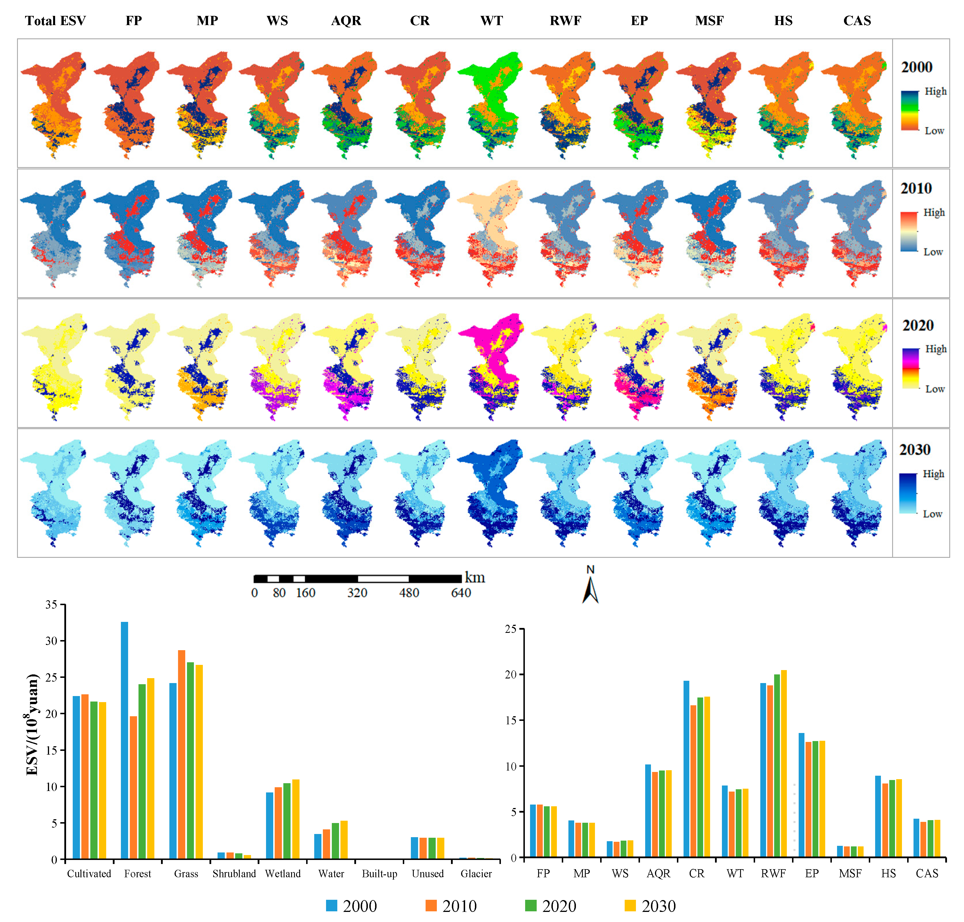
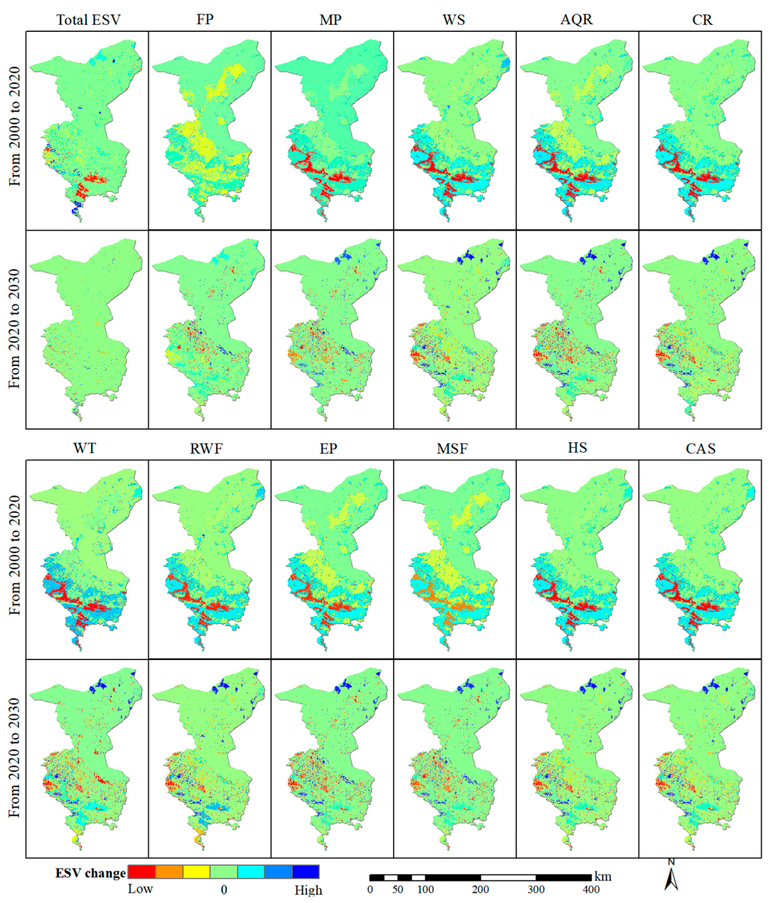
The analysis revealed that the ESV of Wuwei Oasis experienced a decline of 6.96 × 10⁸ from 2000 to 2010, and while the area experienced a partial recovery from 2010 to 2020, the rate of recovery was slower than the decline from 2000 to 2010 (Figure 4 and Figure 5). Furthermore, the ESV of this study’s area remained in a state of loss from 2000 to 2020, with a slight increase predicted for 2030.

4.2.1. Contribution of Different Ecosystem Services to ESV

In terms of the contribution of different ecosystem services to ESV, climate regulation and regulation of water flows were the main types of ecosystem services in Wuwei Oasis, accounting for 20.11% and 19.84% of the total ESV, respectively. In contrast, water supply and maintenance of soil fertility had the smallest proportions, only 1.83% and 1.31%, respectively. During the period from 2000 to 2010, all ecosystem services exhibited a decreasing trend, with the highest loss rates for climate regulation services (−0.71%). From 2010 to 2020, except for food production, all ES exhibited an increasing trend, although with a small overall growth rate. Among them, water supply had the highest ESV growth rate of 0.71%, while food production had a loss rate of −0.31%. From 2000 to 2020, except for the regulation of water flows and water supply, all other ecosystem services led to ESV losses. The ESV changes from 2020 to 2030 were consistent with those from 2010 to 2020, with an increasing trend for all ecosystem services except food production. However, the loss rate of food production was low, and the regulation of water flows had the highest growth rate. Qualitatively, the distribution pattern of ESV increased gradually from northeast to southwest, which was attributed to the distribution of land use types from unused land, cultivated land, and grassland to forest from northeast to southwest, with a corresponding increase in vegetation cover. The 11 ESV types exhibited differences and similarities, with similarities in their spatial distribution patterns, while differences mainly reflected the composition of different ecosystem services. High values of the total ESV were relatively scarce, scattered in Tianzhu in the south. The 11 types of ESV could be divided into three categories. The first category included food production, material production, air quality regulation, erosion prevention, and maintenance of soil fertility, with relatively balanced high, medium, and low-value areas. The high-value areas were mainly distributed in the central part of Minqin, the southern parts of Liangzhou and Gulang, and the northern part of Tianzhu. The low-value areas surrounded the high-value areas, and the medium-value areas were only present in the southern part of Tianzhu. The second category included water supply, climate regulation, regulation of water flows, habitat services, and cultural and amenity services, where some high-value areas in the first category were replaced by medium-value areas in the second category, indicating that the functions of the second category of ecosystem services were lower than those of the first category. The third category was water treatment, which differed from the second category in that medium-value areas replaced high-value areas, indicating that water treatment in Minqin had stronger functional capabilities than the above services.

4.2.2. Contribution of Different Land Use Types to ESV

The examination of ESV from the perspective of land use types revealed a notable trend in forestland, wetland, and water, which all showed an increase from 2000 to 2010. However, the ESV represented by the remaining land use types exhibited a decrease, with shrubland and glaciers experiencing the highest loss rate of ESV (−1.37% and −2.38%, respectively). The ESV changes observed from 2010 to 2020 remained consistent with the trend from 2000 to 2010, except for unused land, which changed from a decline to an increase. Over the entire 20-year period from 2000 to 2020, forests experienced the most severe loss of ESV. Looking ahead to 2030, the distribution of ESV in Wuwei Oasis is expected to be the lowest in the edge area of Minqin, which is consistent with the spatial distribution of unused land. Additionally, the forest in Tianzhu contributed the most to ESV. Among the ESVs represented by different land use types, grassland, wetland, and water all showed a decreasing trend, with water having the largest loss rate of ESV (−3.45%) and shrubland having the highest growth rate (6.32%).

4.3. Ecological Compensation Changes from 2000 to 2030

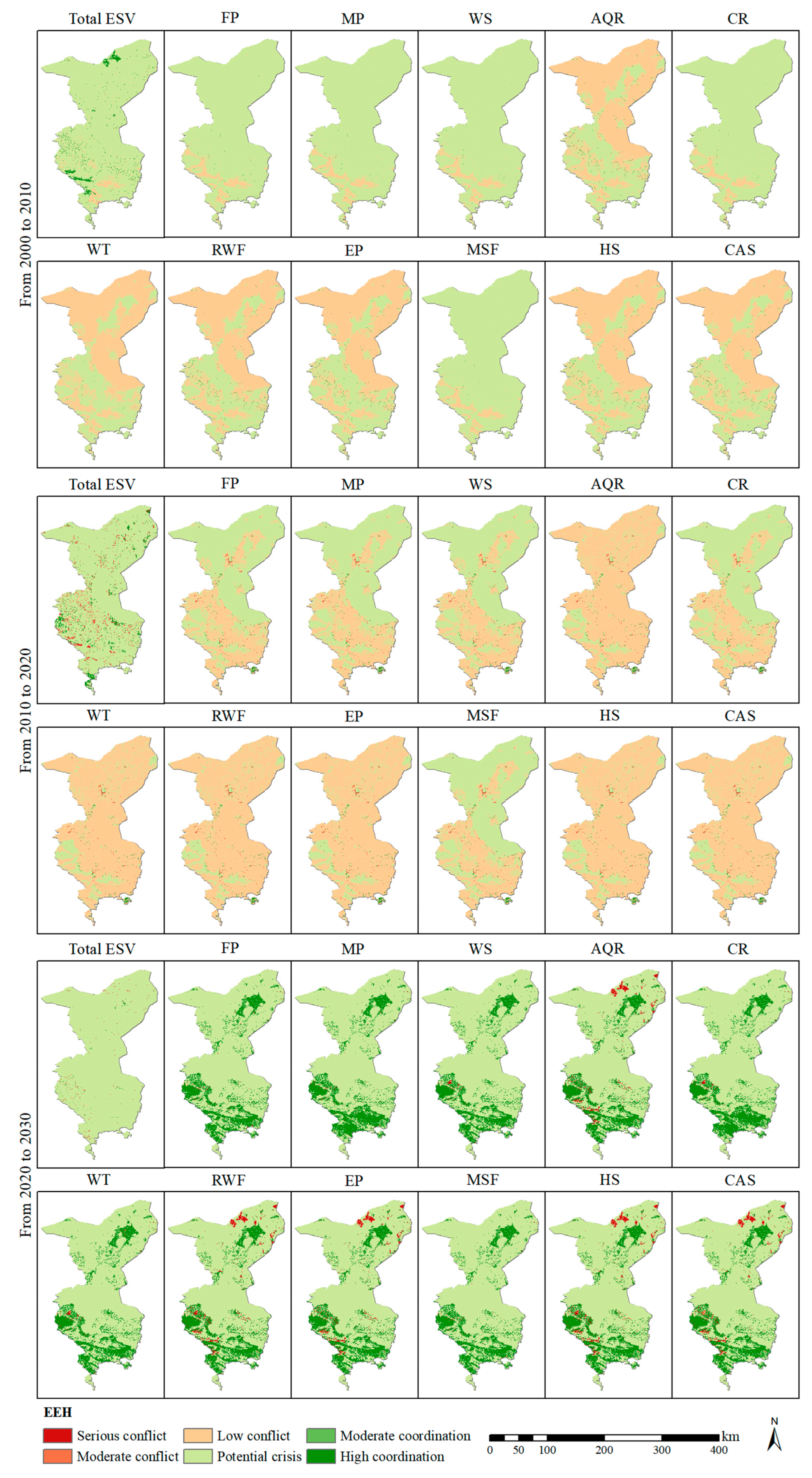
There are significant differences in the temporal and spatial distributions of total EEH and different ecosystem services’ EEH (Figure 6). From a temporal perspective, this study identified five types of EEH from 2000 to 2010, including moderate conflict, low conflict, potential crisis, moderate coordination, and high coordination. The overall study area exhibited a potential crisis, with highly coordinated areas in the Northern Minqin and Northwestern Tianzhu, suggesting that the changes in ESV and GDP were positively correlated during this period. In contrast, Southeastern Tianzhu showed low conflict, indicating that economic development had caused some loss of ESV and had an impact on the ecological environment. From 2010 to 2020, the EEH types remained consistent with those from 2000 to 2010, but the proportion of moderate and high conflict and coordination increased. In the 2020–2030 EEH types, high conflict replaced moderate conflict, and coordination shifted toward a negative direction. The ecological and economic status of this study’s area underwent a shift from coordination to contradiction and then back to coordination due to the rapid population growth and negative growth of ESV from 2010 to 2020, leading to a lower level of conflict between the ecological environment and economic development.

Although the total EEH changes were relatively peaceful, the EEH changes in different ecosystem services were more intense. Specifically, from 2000 to 2020, the potential crisis turned into low conflict. From 2010 to 2030, the contradiction and coordination status became more apparent. The strong coordination is mainly due to the high altitude of these areas, which partly limited the regional economic development. However, a large amount of water and grass resources provided a higher ESV, indicating a high demand for ecological compensation in the area. Therefore, priority should be given to ecological compensation to promote the common development of ecology and economy. The more apparent the contradiction, the more serious the ecological degradation problem, and resolving the contradiction should be the main way to solve the problem, with ecological compensation as an auxiliary tool. As time passes, the gap in ecological compensation priority is gradually increasing, indicating that the economic development level gap between counties is gradually widening. Thus, focus on addressing the ecological degradation problems related to air quality regulation, regulation of water flows, erosion prevention, habitat services, and cultural and amenity services. Meanwhile, to deal with the widening gap between counties, ecological compensation should be given priority to Tianzhu, followed by Minqin, Gulang, and Liangzhou.

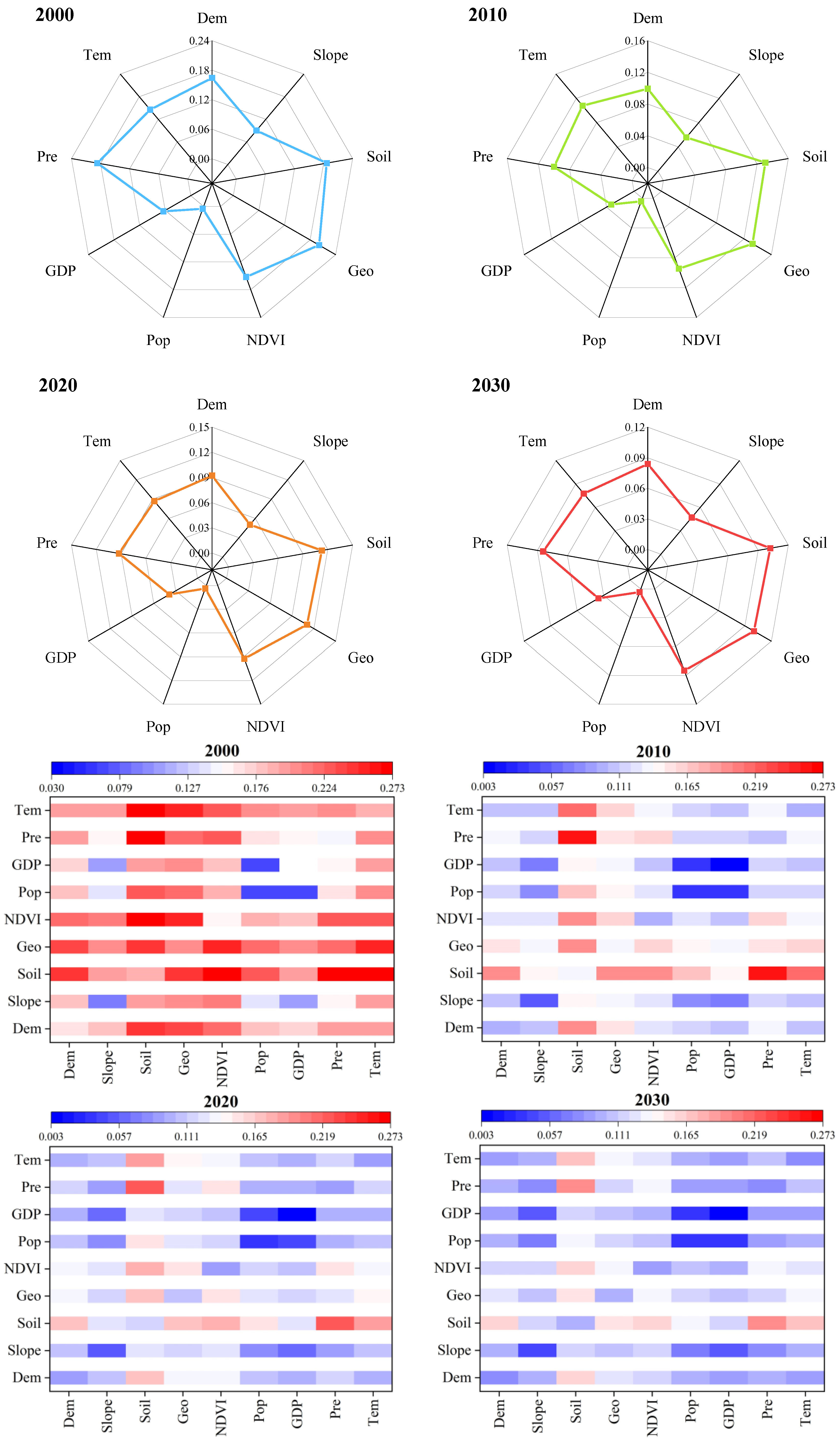
4.4. Driving Mechanism of ESV

We found that the impact trends of driving factors on ESV were consistent across different years, with an overall decreasing trend from 2000 to 2030 (Figure 7). Among the natural, socio-economic, and climatic factors considered, the geomorphic type had the highest q value, followed by soil type and DEM. Geomorphic, soil, and DEM were identified as the primary driving factors affecting regional ESV. This was because this study’s area is located in an ecologically sensitive area with significant spatial differences in terrain. Our findings suggest that elevation plays an important role in the spatial distribution of ESV in the arid oasis area. Climate factors mainly affected the material exchange between underground soil and aboveground vegetation through changes in precipitation and temperature, ultimately impacting changes in regional ESV. In contrast, the socio-economic factors had the weakest driving force. The population density represented the degree of disturbance of human activities on ESV. The q value for GDP was the lowest, indicating that its impact on the spatial differentiation of ESV was the smallest. The low contribution rate of population density and GDP in the area was mainly due to the small proportion of urban areas and population distribution in this study’s area. This is consistent with previous research, but the driving mechanisms of ESV differ significantly between the arid oasis area and the humid coastal area of Southeast China. In the humid southeast area, socio-economic factors such as GDP and population density are the main driving forces behind the loss of ESV, while in the northwest arid area, the increase in ESV is mainly driven by natural landscape patterns. This corresponds to the significant differences in socio-economic development and natural landscape between the humid southeast area and the arid northwest area.

The results of exploring the interactions between factors showed that the driving factors had a synergistic and enhancing effect on ESV in the Wuwei Oasis. Specifically, there were two distinct modes of interaction, nonlinear enhancement, and two-factor enhancement. The results of two-factor interactions were consistent with those of single-factor interactions, with q values showing a decreasing trend from 2000 to 2030. However, the contribution of two-factor interactions was significantly higher than that of single-factor interactions, indicating a significant enhancement effect on the spatial differentiation of ESV. Notably, the interaction between natural factors and other factors had the most significant effect on ESV, with the q values exceeding the average value. Specifically, the interaction between geomorphic type and other factors had the greatest driving force.

5. Discussion

5.1. Model Advantages

The neighborhood effect plays a critical role in extracting transfer rules and calculating conversion probabilities in the dynamic simulation of the urban expansion [24,55]. Extracting temporal features is an essential part of this process, which determines the dependency relationships between model variables and parameters by computing gradients and storing them through a time-backward propagation [56]. Recurrent Neural Network (RNN) can pass the output and state of the current time as inputs to the next time, maintaining the data relationship between each time, and has been proven to be an effective deep learning model for processing time-series data [57]. However, RNN faces challenges such as vanishing and exploding gradients, which limit their ability to maintain long-term dependencies. Many excellent evolutionary models have been developed to optimize RNN, such as LSTM and GRU. LSTM adds memory units to address long-term dependency issues [58], while GRU reduces computational tensors by combining forget gates and input gates into a single update gate [52]. GRU also mixes cell states and hidden states, making the model more efficient and faster to train [59]. Applying batch normalization to the model optimizes the distribution width and offset, accelerates the network learning rate, and facilitates the gradient propagation [60]. ReLU, as an activation function, has sparse activation properties, enabling it to learn relatively sparse features from effective data dimensions and automatically decouple features to avoid overfitting [61]. In the context of abundant and comprehensive data, our model effectively harnesses regional land use data, in conjunction with key natural geographic and socio-economic factors, to undergo rigorous learning and training processes, iteratively fine-tuning various hyperparameters to achieve optimal performance. Although this study focused on a specific region, the model’s underlying principles and methodologies were designed to be adaptable to different climatic zones. By carefully considering the environmental and socio-economic characteristics of various regions during model calibration and validation, this model’s accuracy and reliability can be enhanced for use in diverse geographical contexts. Consequently, the applicability of this model extends beyond arid and semi-arid regions, encompassing a broader spectrum of climate zones, including humid and semi-humid areas.

Previous studies on the spatiotemporal variation of ESV have mainly focused on statistical analysis of quantitative data, with limited investigations on the underlying mechanisms driven by spatial factors. GeoDetector is highly inclusive in their analysis of data features. On the one hand, it can directly analyze quantified numerical values such as temperature and precipitation, which influence ecosystem services by regulating water and heat conditions and affecting biological behavior [62,63,64]. Additionally, socioeconomic factors such as GDP and population density directly impact ESV through human activities [65]. On the other hand, it quantifies qualitative numerical values before analysis. For example, natural factors such as soil type and geomorphic type, as the background elements of biological habitat in the ecosystem, have important functions in accumulating organic carbon and promoting water cycling. Changes in the background ecological conditions have a substantial impact on ecosystem services such as soil conservation, soil erosion, and biodiversity [66].

5.2. Relationship between Land Use and ESV

Between 2000 to 2020, hydrological regulation remained the dominant function in this study’s area. By 2030, climate regulation will surpass hydrological regulation to become the dominant function in the arid oasis area of Wuwei. Despite this change, the proportion of most ecosystem service functions remained stable with no more than a 0.005 change, indicating a relatively stable structure of ecosystem service functions. Food production and soil erosion experienced the most significant decrease in proportion, while hydrological regulation increased by 0.009. This transformation primarily occurred in areas with more intense human activities, which aligns with the resource utilization characteristics in China’s arid areas [67,68]. Qualitatively, the ESV of various ecosystem services in this study’s area exhibited slight changes between 2000 and 2030, which can be visually observed in Figure 4. By comparison, the spatial distribution of ESV changes in the first 20 years was generally more drastic than those in the future 10 years, with continuous changes in the former and scattered changes in the latter. From 2000 to 2020, the degradation areas of food production, material production, air quality regulation, erosion prevention, and maintenance of soil fertility accounted for the largest proportion. The proportion of ESV losses and gains of other ecosystem services was relatively average. Although the distribution of ESV changes varied slightly among different ecosystem services, the spatial distribution changes in ESV for ecosystem services were generally greater than the overall ESV amplitude. This complexity underscores the importance of studying ESV characterization for different ecosystem services.

Land use change is a complex dynamic process that can have direct or indirect impacts on ecosystem services and ESV [69]. The increase or decrease in ESV in this study area is mainly contributed by farmland, forest, and grassland. Urban expansion, in particular, has occupied a considerable amount of ecological land, leading to a deterioration of the coupling coordination relationship between urban expansion and food production function. This phenomenon has caused varying degrees of damage to the original functions of the ecosystem, resulting in the problem of high-speed and low-quality urban expansion [70]. Due to natural geographic conditions, cultivated land is the most commonly occupied land type during urban expansion. The rapid reduction in cultivated land area disrupts the balanced ecological process and leads to a decline in the ecological system’s food production value [71,72]. However, high-ESV land types, such as forests, wetlands, and water bodies, are the main drivers of ESV changes because their ESV per unit area is higher than that of cultivated land.

While previous research by Long, et al. [73] has shown that land use change due to urban expansion in the eastern coastal area of China has severely damaged the ecosystem and resulted in a decrease in ESV; our quantitative analysis of the Wuwei Oasis area’s ESV indicates an opposite trend over time. This discrepancy can be attributed to differences in climate, topography, urban expansion speed, and ecological environment between the arid northwest area and the southeastern coastal area. To promote the sustainable development of such eco-fragile cities as Wuwei Oasis, it is essential to plan regional land use reasonably and optimize both economic and ecological benefits. Built-up land can reduce the ESV of this study’s area, while the increase in ecological land, such as water bodies, wetlands, and forests, will lead to an increase in ESV. Therefore, optimizing both economic and ecological benefits, reducing ESV losses caused by unregulated development, and protecting land use types with high ESV are the most effective ways to increase ESV [74].

5.3. Insights and Recommendations on Ecological Compensation

In reality, ecological compensation schemes in arid oasis areas are still in their early stages, making the EEH prediction of ESV and its ecological compensation priority practically significant. ESV is a composite measure of diverse ecosystem services, including provisioning, regulating, supporting, and cultural services. Unfortunately, current research has only focused on total ESV policy and has not fully expressed the relationship between ESV and the various ecosystem services [75,76]. Based on the EEH prediction results of Wuwei in the arid oasis area, we propose suggestions for its sustainable development. Firstly, measures must be taken to alleviate the degradation of air quality regulation, hydrological regulation, soil retention, biodiversity, and cultural services in Tianzhu and Minqin. The main way is to increase vegetation coverage through afforestation to neutralize carbon emissions in the atmosphere. It is also possible to prevent natural disasters such as drought, floods, and debris flow to prevent large-scale soil and water loss and to designate ecological protection zones to prevent the extinction of rare animals and plants. Secondly, to further quantify ecological compensation standards in the arid oasis area, the ESV, characterized by 11 ecosystem services, should be divided into natural contribution, human input, human preference, and natural contribution + human input, based on their importance and differences. Furthermore, our study has explored the driving factors of total ESV; natural and human factors also have certain impacts on ecosystem services. For example, a large terrain relief or excessive rainfall will accelerate surface runoff velocity, enhance soil erosion, and cause soil and water loss. A higher vegetation coverage of forest or grassland with certain canopy closures can reduce soil erosion and increase hydrological regulation and soil conservation ability. Unreasonable land use by humans may destroy surface vegetation and stable terrain, leading to the degradation of ecosystem services. Therefore, targeted exploration of the driving mechanisms of ESV characterized by different ecosystem services should be conducted to promote ecological and economic coordinated sustainable development.

5.4. Limitations and Future Perspectives

In this study, we employed a high-performance deep learning model to simulate the future ESV and ecological compensation in arid regions. The conducted investigation offers valuable practical implications for land use planning and ecological compensation policies. The main findings of this study are attractive for various regions and countries facing similar challenges in land use management and ecological compensation. The deep learning model’s transferability can be evaluated by adapting it to different study areas and considering region-specific data and contextual factors [77]. In addition, the advanced land use simulation and geospatial analysis techniques facilitate the identification of ecologically sensitive areas, potential conflicts between economic development and environmental conservation, and opportunities for ecological compensation schemes [78]. The insights gained from our research can be utilized to inform policy development and land use planning in diverse geographic contexts.

However, it is crucial to acknowledge the inherent limitations of our research. Firstly, our land use simulation did not encompass multiple scenarios. While the baseline scenario captures one potential future development trajectory, the implementation of novel ecological and economic policies could exert notable influences on land use dynamics. As a result, future investigations could integrate historical trends of land use changes and pertinent policy considerations to furnish scientific underpinnings for territorial spatial planning and the advancement of sustainable urban development. By accounting for a broader range of scenarios, more comprehensive insights into the complex interplay between human activities and ecological systems can be attained, enhancing the utility and robustness of our findings. Moreover, further efforts in data collection and model refinement could aid in reducing uncertainties and refining the precision of our predictions, ensuring greater accuracy and applicability in decision-making processes and policy formulation.

6. Conclusions

Through the application of deep learning models and spatial analysis methods, this study provides valuable insights into the identification of priority areas for ecological compensation and the driving factors contributing to ESV in arid oasis areas. Results demonstrate that (1) Deep learning models effectively captured the spatiotemporal neighborhood features of land use dynamics, and CNN-GRU exhibited the highest accuracy and most accurately simulated the 2020 land use; (2) The built-up area of Wuwei Oasis is projected to increase by 25.35% from 2000 to 2030, resulting in a significant decline in ESV (−2.38%). Climate regulation was identified as the main contributor to ESV in this study, while the loss rate was also the highest. Wetlands and water bodies were the dominant factors affecting the change in ESV per area unit; (3) In the historical period, EEH was primarily characterized by low conflicts and potential crises, while potential crises and high coordination will be the main features in the future. The coordination of Minqin and Tianzhu in the south and north of this study’s area was generally higher than that of Liangzhou and Guluang in the east and west, and the urgency of ecological compensation was correspondingly higher; (4) Natural factors had the most significant impact on ESV, and the explanatory power of bivariate interaction detection for ESV spatial differentiation increased significantly. Moreover, the contribution of single and multiple factors to ESV showed a decreasing trend from 2000 to 2030. Overall, the findings of this study provide important insights that can inform strategies for promoting the restoration of oasis ecosystems and sustainable urban development.

References

1. Lu, Y.; Fu, B.; Feng, X.; Zeng, Y.; Liu, Y.; Chang, R.; Sun, G.; Wu, B. A Policy-Driven Large Scale Ecological Restoration: Quantifying Ecosystem Services Changes in the Loess Plateau of China. PLoS ONE 2012, 7, e31782. [Google Scholar] [CrossRef] [Green Version]
2. Wang, Y.; Li, X.; Zhang, Q.; Li, J.; Zhou, X. Projections of future land use changes: Multiple scenarios -based impacts analysis on ecosystem services for Wuhan city, China. Ecol. Indic. 2018, 94, 430–445. [Google Scholar] [CrossRef]
3. He, C.; Liu, Z.; Tian, J.; Ma, Q. Urban expansion dynamics and natural habitat loss in China: A multiscale landscape perspective. Glob. Chang. Biol. 2014, 20, 2886–2902. [Google Scholar] [CrossRef] [PubMed]
4. Zhang, D.; Wang, X.; Qu, L.; Li, S.; Lin, Y.; Yao, R.; Zhou, X.; Li, J. Land use/cover predictions incorporating ecological security for the Yangtze River Delta region, China. Ecol. Indic. 2020, 119, 106841. [Google Scholar] [CrossRef]
5. Mirbagheri, B.; Alimohammadi, A. Improving urban cellular automata performance by integrating global and geographically weighted logistic regression models. Trans. Gis 2017, 21, 1280–1297. [Google Scholar] [CrossRef]
6. Seto, K.C.; Gueneralp, B.; Hutyra, L.R. Global forecasts of urban expansion to 2030 and direct impacts on biodiversity and carbon pools. Proc. Natl. Acad. Sci. USA 2012, 109, 16083–16088. [Google Scholar] [CrossRef]
7. McDonald, R.I.; Guneralp, B.; Huan, C.-W.; Seto, K.C.; You, M. Conservation priorities to protect vertebrate endemics from global urban expansion. Biol. Conserv. 2018, 224, 290–299. [Google Scholar] [CrossRef]
8. Fensholt, R.; Langanke, T.; Rasmussen, K.; Reenberg, A.; Prince, S.D.; Tucker, C.; Scholes, R.J.; Le, Q.B.; Bondeau, A.; Eastman, R.; et al. Greenness in semi-arid areas across the globe 1981-2007—An Earth Observing Satellite based analysis of trends and drivers. Remote Sens. Environ. 2012, 121, 144–158. [Google Scholar] [CrossRef]
9. Tan, Z.; Guan, Q.; Lin, J.; Yang, L.; Luo, H.; Ma, Y.; Tian, J.; Wang, Q.; Wang, N. The response and simulation of ecosystem services value to land use/land cover in an oasis, Northwest China. Ecol. Indic. 2020, 118, 106711. [Google Scholar] [CrossRef]
10. Abulizi, A.; Yang, Y.; Mamat, Z.; Luo, J.; Abdulslam, D.; Xu, Z.; Zayiti, A.; Ahat, A.; Halik, W. Land-Use Change and its Effects in Charchan Oasis, Xinjiang, China. Land Degrad. Dev. 2017, 28, 106–115. [Google Scholar] [CrossRef]
11. Fu, Q.; Li, B.; Hou, Y.; Bi, X.; Zhang, X. Effects of land use and climate change on ecosystem services in Central Asia’s arid regions: A case study in Altay Prefecture, China. Sci. Total Environ. 2017, 607, 633–646. [Google Scholar] [CrossRef]
12. Zhang, T.; Du, Z.; Yang, J.; Yao, X.; Ou, C.; Niu, B.; Yan, S. Land Cover Mapping and Ecological Risk Assessment in the Context of Recent Ecological Migration. Remote Sens. 2021, 13, 1381. [Google Scholar] [CrossRef]
13. Guan, Q.; Zhao, R.; Pan, N.; Wang, F.; Yang, Y.; Luo, H. Source apportionment of heavy metals in farmland soil of Wuwei, China: Comparison of three receptor models. J. Clean. Prod. 2019, 237, 117792. [Google Scholar] [CrossRef]
14. Kindu, M.; Schneider, T.; Doellerer, M.; Teketay, D.; Knoke, T. Scenario modelling of land use/land cover changes in Munessa-Shashemene landscape of the Ethiopian highlands. Sci. Total Environ. 2018, 622, 534–546. [Google Scholar] [CrossRef] [PubMed]
15. Zhu, S.; Zhao, Y.; Huang, J.; Wang, S. Analysis of Spatial-Temporal Differentiation and Influencing Factors of Ecosystem Services in Resource-Based Cities in Semiarid Regions. Remote Sens. 2023, 15, 871. [Google Scholar] [CrossRef]
16. Zhou, T.; Chen, W.; Wang, Q.; Li, Y. Urbanisation and ecosystem services in the Taiwan Strait west coast urban agglomeration, China, from the perspective of an interactive coercive relationship. Ecol. Indic. 2023, 146, 109861. [Google Scholar] [CrossRef]
17. Wu, Y.; Tao, Y.; Yang, G.; Ou, W.; Pueppke, S.; Sun, X.; Chen, G.; Tao, Q. Impact of land use change on multiple ecosystem services in the rapidly urbanizing Kunshan City of China: Past trajectories and future projections. Land Use Policy 2019, 85, 419–427. [Google Scholar] [CrossRef]
18. Li, F.; Wang, L.; Chen, Z.; Clarke, K.C.; Li, M.; Jiang, P. Extending the SLEUTH model to integrate habitat quality into urban growth simulation. J. Environ. Manag. 2018, 217, 486–498. [Google Scholar] [CrossRef] [Green Version]
19. Zhang, D.; Huang, Q.; He, C.; Wu, J. Impacts of urban expansion on ecosystem services in the Beijing-Tianjin-Hebei urban agglomeration, China: A scenario analysis based on the Shared Socioeconomic Pathways. Resour. Conserv. Recycl. 2017, 125, 115–130. [Google Scholar] [CrossRef]
20. Xiao, R.; Yu, X.; Zhang, Z.; Wang, X. Built-up land expansion simulation with combination of naive Bayes and cellular automaton model-A case study of the Shanghai-Hangzhou Bay agglomeration. Growth Chang. 2021, 52, 1804–1825. [Google Scholar] [CrossRef]
21. Wu, Q.; Guan, F.; Lv, C.; Huang, Y. Ultra-short-term multi-step wind power forecasting based on CNN-LSTM. IET Renew. Power Gener. 2021, 15, 1019–1029. [Google Scholar] [CrossRef]
22. Wang, H.; Zhao, X.; Zhang, X.; Wu, D.; Du, X. Long Time Series Land Cover Classification in China from 1982 to 2015 Based on Bi-LSTM Deep Learning. Remote Sens. 2019, 11, 1639. [Google Scholar] [CrossRef] [Green Version]
23. Zhai, Y.; Yao, Y.; Guan, Q.; Liang, X.; Li, X.; Pan, Y.; Yue, H.; Yuan, Z.; Zhou, J. Simulating urban land use change by integrating a convolutional neural network with vector-based cellular automata. Int. J. Geogr. Inf. Sci. 2020, 34, 1475–1499. [Google Scholar] [CrossRef]
24. Qian, Y.; Xing, W.; Guan, X.; Yang, T.; Wu, H. Coupling cellular automata with area partitioning and spatiotemporal convolution for dynamic land use change simulation. Sci. Total Environ. 2020, 722, 137738. [Google Scholar] [CrossRef]
25. Liu, J.; Xiao, B.; Li, Y.; Wang, X.; Jiao, J. Simulation of Dynamic Urban Expansion under Ecological Constraints Using a Long Short Term Memory Network Model and Cellular Automata. Remote Sens. 2021, 13, 1499. [Google Scholar] [CrossRef]
26. Cao, J.; Wang, Y.; He, J.; Liang, W.; Tao, H.; Zhu, G. Predicting Grain Losses and Waste Rate Along the Entire Chain: A Multitask Multigated Recurrent Unit Autoencoder Based Method. IEEE Trans. Ind. Inform. 2021, 17, 4390–4400. [Google Scholar] [CrossRef]
27. Chen, Z.; Xia, T.; Li, Y.; Pan, E. A hybrid prognostic method based on gated recurrent unit network and an adaptive Wiener process model considering measurement errors. Mech. Syst. Signal Process. 2021, 158, 107785. [Google Scholar] [CrossRef]
28. Gao, X.; Zeng, S.; Shen, J.; Yang, X.; Kang, L.; Chi, C.; Song, R. Predicting payment for ecosystem services regarding land use: A simulation study in China. Environ. Impact Assess. Rev. 2023, 98, 106972. [Google Scholar] [CrossRef]
29. Ren, Y.; Lu, L.; Yu, H.; Zhu, D. Game strategies in government-led eco-compensation in the Xin’an River Basin from the perspective of the politics of scale. J. Geogr. Sci. 2021, 31, 1205–1221. [Google Scholar] [CrossRef]
30. Jiang, Y.; Zhang, J.; Chen, K.; Xue, X.; Michael, A.U. Moving towards a systematic marine eco-compensation mechanism in China: Policy, practice and strategy. Ocean. Coast. Manag. 2019, 169, 10–19. [Google Scholar] [CrossRef]
31. Wu, L.; Jin, L. How eco-compensation contribute to poverty reduction: A perspective from different income group of rural households in Guizhou, China. J. Clean. Prod. 2020, 275, 122962. [Google Scholar] [CrossRef]
32. Xie, Y.; Kong, F.; Zhang, J.; Li, Y.; Huang, G.; Zhang, W. Medium- and Long-Term Planning of an Integrated Eco-Compensation System Considering Ecological Water Demand under Uncertainty: A Case Study of Daguhe Watershed in China. J. Water Resour. Plan. Manag. 2022, 148, 04022049. [Google Scholar] [CrossRef]
33. Xiao, W.; Qu, L.; Li, K.; Guo, C.; Li, J. An Assessment of the Rational Range of Eco-Compensation Standards: A Case Study in the Nujiang Prefecture, Southwestern China. Land 2022, 11, 1417. [Google Scholar] [CrossRef]
34. Liu, R.; Xu, H.; Li, J.; Pu, R.; Sun, C.; Cao, L.; Jiang, Y.; Tian, P.; Wang, L.; Gong, H. Ecosystem service valuation of bays in East China Sea and its response to sea reclamation activities. J. Geogr. Sci. 2020, 30, 1095–1116. [Google Scholar] [CrossRef]
35. Wang, Z.; Wang, Y.; Zhou, Z.; Yu, F.; Ma, D.; Li, J. Combining spatial planning and ecosystem services value to assist ecological compensation decision-making-A case study of Yangtze River Delta ecological barrier, China. Front. Environ. Sci. 2022, 10, 1002014. [Google Scholar] [CrossRef]
36. Liu, Z.; Wu, R.; Chen, Y.; Fang, C.; Wang, S. Factors of ecosystem service values in a fast-developing region in China: Insights from the joint impacts of human activities and natural conditions. J. Clean. Prod. 2021, 297, 126588. [Google Scholar] [CrossRef]
37. Chen, S.; Feng, Y.; Tong, X.; Liu, S.; Xie, H.; Gao, C.; Lei, Z. Modeling ESV losses caused by urban expansion using cellular automata and geographically weighted regression. Sci. Total Environ. 2020, 712, 136509. [Google Scholar] [CrossRef] [PubMed]
38. Luo, Q.; Luo, Y.; Zhou, Q.; Song, Y. Does China’s Yangtze River Economic Belt policy impact on local ecosystem services? Sci. Total Environ. 2019, 676, 231–241. [Google Scholar] [CrossRef]
39. Song, W.; Deng, X. Land-use/land-cover change and ecosystem service provision in China. Sci. Total Environ. 2017, 576, 705–719. [Google Scholar] [CrossRef]
40. Zhang, X.; Li, H.; Xia, H.; Tian, G.; Yin, Y.; Lei, Y.; Kim, G. The Ecosystem Services Value Change and Its Driving Forces Responding to Spatio-Temporal Process of Landscape Pattern in the Co-Urbanized Area. Land 2021, 10, 1043. [Google Scholar] [CrossRef]
41. Chen, M.; Lu, Y.; Ling, L.; Wan, Y.; Luo, Z.; Huang, H. Drivers of changes in ecosystem service values in Ganjiang upstream watershed. Land Use Policy 2015, 47, 247–252. [Google Scholar] [CrossRef]
42. Huang, M.; Fang, B.; Yue, W.; Feng, S. Spatial differentiation of ecosystem service values and its geographical detection in Chaohu Basin during 1995–2017. Acta Geogr. Sin. 2019, 38, 2790–2803. [Google Scholar]
43. Wang, J.; Xu, C. Geodetector: Principle and prospective. Acta Geogr. Sin. 2017, 72, 19. [Google Scholar]
44. Wang, J.F.; Hu, Y. Environmental health risk detection with GeogDetector. Environ. Model. Softw. 2012, 20, 114–115. [Google Scholar] [CrossRef]
45. Liu, X.; Chen, X.; Hua, K.; Wang, Y.; Wang, P.; Han, X.; Ye, J.; Wen, S. Effects of Land Use Change on Ecosystem Services in Arid Area Ecological Migration. Chin. Geogr. Sci. 2018, 28, 894–906. [Google Scholar] [CrossRef] [Green Version]
46. Bauer, S. Identification of Water-Reuse Potentials to Strengthen Rural Areas in Water-Scarce Regions-The Case Study of Wuwei. Land 2020, 9, 492. [Google Scholar] [CrossRef]
47. Kadulkar, S.; Howard, M.P.; Truskett, T.M.; Ganesan, V. Prediction and Optimization of Ion Transport Characteristics in Nanoparticle-Based Electrolytes Using Convolutional Neural Networks. J. Phys. Chem. B 2021, 125, 4838–4849. [Google Scholar] [CrossRef]
48. Fei, X.; Zhang, Y.; Zheng, W. XB-SIM*: A Simulation Framework for Modeling and Exploration of ReRAM-Based CNN Acceleration Design. Tsinghua Sci. Technol. 2021, 26, 322–334. [Google Scholar] [CrossRef]
49. Xie, J.; Chen, S.; Zhang, Y.; Gao, D.; Liu, T. Combining generative adversarial networks and multi-output CNN for motor imagery classification. J. Neural Eng. 2021, 18, 046026. [Google Scholar] [CrossRef]
50. Rehman, S.U.; Khaliq, M.; Imtiaz, S.I.; Rasool, A.; Shafiq, M.; Javed, A.R.; Jalil, Z.; Bashir, A.K. DIDDOS: An approach for detection and identification of Distributed Denial of Service (DDoS) cyberattacks using Gated Recurrent Units (GRU). Future Gener. Comput. Syst. 2021, 118, 453–466. [Google Scholar] [CrossRef]
51. Huang, N.; Nie, F.; Ni, P.; Luo, F.; Gao, X.; Wang, J. NeuralPolish: A novel Nanopore polishing method based on alignment matrix construction and orthogonal Bi-GRU Networks. Bioinformatics 2021, 37, 3120–3127. [Google Scholar] [CrossRef] [PubMed]
52. Huang, G.; Li, X.; Zhang, B.; Ren, J. PM2.5 concentration forecasting at surface monitoring sites using GRU neural network based on empirical mode decomposition. Sci. Total Environ. 2021, 768, 144516. [Google Scholar] [CrossRef] [PubMed]
53. Xie, G.; Zhang, C.; Zhen, L.; Zhang, L. Dynamic changes in the value of China’s ecosystem services. Ecosyst. Serv. 2017, 26, 146–154. [Google Scholar] [CrossRef]
54. Wang, X.; Xu, M.; Zhang, Y.; Xu, N.; Zhang, Y. Evaluation of Eco-economy Harmony and Spatial Evolution of the Urban Agglomeration Area in The Great Pearl River Delta. In Proceedings of the 2nd International Workshop on Renewable Energy and Development (IWRED), Guilin, China, 20–22 April 2018. [Google Scholar] [CrossRef]
55. Liao, J.; Tang, L.; Shao, G.; Su, X.; Chen, D.; Xu, T. Incorporation of extended neighborhood mechanisms and its impact on urban land-use cellular automata simulations. Environ. Model. Softw. 2016, 75, 163–175. [Google Scholar] [CrossRef] [Green Version]
56. Aburas, M.M.; Ahamad, M.S.S.; Omar, N.Q. Spatio-temporal simulation and prediction of land-use change using conventional and machine learning models: A review. Environ. Monit. Assess. 2019, 191, 205. [Google Scholar] [CrossRef]
57. Liu, L.; Sun, X.-K. Volcanic Ash Cloud Diffusion From Remote Sensing Image Using LSTM-CA Method. IEEE Access 2020, 8, 54681–54690. [Google Scholar] [CrossRef]
58. Jia, X.; Khandelwal, A.; Nayak, G.; Gerber, J.; Carlson, K.; West, P.; Kumar, V. Incremental Dual-Memory LSTM in Land Cover Prediction; ACM: New York, NY, USA, 2017; pp. 867–876. [Google Scholar]
59. Yan, L.; Wang, H.; Wang, H.; Liu, Z. An integrated GRU based real-time prognostic method towards uncertainty quantification. Meas. Sens. 2021, 18, 100220. [Google Scholar] [CrossRef]
60. Lian, J.; Dong, P.; Zhang, Y.; Pan, J.; Liu, K. A Novel Data-Driven Tropical Cyclone Track Prediction Model Based on CNN and GRU With Multi-Dimensional Feature Selection. IEEE Access 2020, 8, 97114–97128. [Google Scholar] [CrossRef]
61. Zhang, N.; Zhang, N.; Zheng, Q.; Xu, Y.S. Real-time prediction of shield moving trajectory during tunnelling using GRU deep neural network. Acta Geotech. 2021, 17, 1167–1182. [Google Scholar] [CrossRef]
62. Mina, M.; Bugmann, H.; Cordonnier, T.; Irauschek, F.; Klopcic, M.; Pardos, M.; Cailleret, M. Future ecosystem services from European mountain forests under climate change. J. Appl. Ecol. 2017, 54, 389–401. [Google Scholar] [CrossRef]
63. Braun, D.; de Jong, R.; Schaepman, M.E.; Furrer, R.; Hein, L.; Kienast, F.; Damm, A. Ecosystem service change caused by climatological and non-climatological drivers: A Swiss case study. Ecol. Appl. A Publ. Ecol. Soc. Am. 2019, 29, e01901. [Google Scholar] [CrossRef] [PubMed]
64. Prather, C.M.; Pelini, S.L.; Laws, A.; Rivest, E.; Woltz, M.; Bloch, C.P.; Toro, I.D.; Ho, C.K.; Kominoski, J.; Newbold, T.A.S. Invertebrates, ecosystem services and climate change. Biol. Rev. 2013, 88, 327–348. [Google Scholar] [CrossRef]
65. Su, S.; Li, D.; Hu, Y.; Xiao, R.; Zhang, Y. Spatially non-stationary response of ecosystem service value changes to urbanization in Shanghai, China. Ecol. Indic. 2014, 45, 332–339. [Google Scholar] [CrossRef]
66. Khl, L.; Oehl, F.; Heijden, M.G.A.V.D. Agricultural practices indirectly influence plant productivity and ecosystem services through effects on soil biota. Ecol. Appl. 2014, 24, 1842–1853. [Google Scholar] [CrossRef] [PubMed]
67. Jiang, W. Ecosystem services research in China: A critical review. Ecosyst. Serv. 2017, 26, 10–16. [Google Scholar] [CrossRef]
68. He, C.; Li, J.; Zhang, X.; Liu, Z.; Zhang, D. Will rapid urban expansion in the drylands of northern China continue: A scenario analysis based on the Land Use Scenario Dynamics-urban model and the Shared Socioeconomic Pathways. J. Clean. Prod. 2017, 165, 57–69. [Google Scholar] [CrossRef]
69. Tripathi, R.; Moharana, K.C.; Nayak, A.D.; Dhal, B.; Shahid, M.; Mondal, B.; Mohapatra, S.D.; Bhattacharyya, P.; Fitton, N.; Smith, P.; et al. Ecosystem services in different agro-climatic zones in eastern India: Impact of land use and land cover change. Environ. Monit. Assess. 2019, 191, 98. [Google Scholar] [CrossRef]
70. Salvati, L.; Zambon, I.; Chelli, F.M.; Serra, P. Do spatial patterns of urbanization and land consumption reflect different socioeconomic contexts in Europe? Sci. Total Environ. 2018, 625, 722–730. [Google Scholar] [CrossRef]
71. Msofe, N.K.; Sheng, L.; Li, Z.; Lyimo, J. Impact of Land Use/Cover Change on Ecosystem Service Values in the Kilombero Valley Floodplain, Southeastern Tanzania. Forests 2020, 11, 109. [Google Scholar] [CrossRef] [Green Version]
72. Rukundo, E.; Liu, S.; Dong, Y.; Rutebuka, E.; Asamoah, E.F.; Xu, J.; Wu, X. Spatio-temporal dynamics of critical ecosystem services in response to agricultural expansion in Rwanda, East Africa. Ecol. Indic. 2018, 89, 696–705. [Google Scholar] [CrossRef]
73. Long, H.; Liu, Y.; Hou, X.; Li, T.; Li, Y. Effects of land use transitions due to rapid urbanization on ecosystem services: Implications for urban planning in the new developing area of China. Habitat Int. 2014, 44, 536–544. [Google Scholar] [CrossRef]
74. Chuai, X.; Huang, X.; Wu, C.; Li, J.; Lu, Q.; Qi, X.; Zhang, M.; Zuo, T.; Lu, J. Land use and ecosystems services value changes and ecological land management in coastal Jiangsu, China. Habitat Int. 2016, 57, 164–174. [Google Scholar] [CrossRef]
75. Fan, H.; Xu, J.; Gao, S. Modeling the dynamics of urban and ecological binary space for regional coordination: A case of Fuzhou coastal areas in Southeast China. Habitat Int. 2018, 72, 48–56. [Google Scholar] [CrossRef]
76. Xing, X.; Yang, X.; Guo, J.; Chen, A.; Zhang, M.; Yang, D.; Hou, Z.; Zhang, H.; Wang, X. Response of ecosystem services in Beijing-Tianjin Sandstorm Source Control Project to differing engineering measures scenarios. J. Clean. Prod. 2023, 384, 135573. [Google Scholar] [CrossRef]
77. van Duynhoven, A.; Dragicevic, S. Assessing the Impact of Neighborhood Size on Temporal Convolutional Networks for Modeling Land Cover Change. Remote Sens. 2022, 14, 4957. [Google Scholar] [CrossRef]
78. Vaissiere, A.-C.; Meinard, Y. A policy framework to accommodate both the analytical and normative aspects of biodiversity in ecological compensation. Biol. Conserv. 2021, 253, 108897. [Google Scholar] [CrossRef]
Figure 1. Study area and land use spatial distribution. Wuwei belongs to a warm-temperate continental arid climate with an average annual temperature of 7.8 °C and a precipitation range of 60–610 mm. In terms of administrative divisions, it includes one district, two counties, and one autonomous county, with a total area of 3.32 × 10⁴ km2.
Remotesensing 15 03927 g001
Figure 2. Research framework. (ESV: ecological service value; FP: food production; MP: material production; WS: water supply; AQR: air quality regulation; CR: climate regulation; WT: waste treatment; RWF: regulation of water flows; EP: erosion prevention; MSF: maintenance of soil fertility; HS: habitat services; CAS: cultural and amenity services).
Remotesensing 15 03927 g002
Figure 3. Simulated and actual land use maps for 2020.
Remotesensing 15 03927 g003
Figure 4. Spatial distribution of total ESV and 11 ESV from 2000 to 2030, and bar graphs are ESVs of different land use types and ecosystem service representations from 2000 to 2030. (FP: food production; MP: material production; WS: water supply; AQR: air quality regulation; CR: climate regulation; WT: waste treatment; RWF: regulation of water flows; EP: erosion prevention; MSF: maintenance of soil fertility; HS: habitat services; CAS: cultural and amenity services).
Remotesensing 15 03927 g004
Figure 5. Spatial distribution changes in total ESV and 11 types of ESV in different periods. Lower variation values correspond to more substantial declines in ESV; higher ESV variation values are indicative of a more pronounced increase in ESV. An ESV variation value of 0 denotes a state of stable ESV, indicating no net change in ESV.
Remotesensing 15 03927 g005
Figure 6. Changes in the spatial distribution of EEH for different ecosystem services in different periods.
Remotesensing 15 03927 g006
Figure 7. The contribution of single-factor (Radar map) and two-factor (Heat map) to ESV.
Remotesensing 15 03927 g007