Vehicle Localization in a Completed City-Scale 3D Scene Using Aerial Images and an On-Board Stereo Camera

Abstract

Simultaneous Localization and Mapping (SLAM) forms the foundation of vehicle localization in autonomous driving. Utilizing high-precision 3D scene maps as prior information in vehicle localization greatly assists in the navigation of autonomous vehicles within large-scale 3D scene models. However, generating high-precision maps is complex and costly, posing challenges to commercialization. As a result, a global localization system that employs low-precision, city-scale 3D scene maps reconstructed by unmanned aerial vehicles (UAVs) is proposed to optimize visual positioning for vehicles. To address the discrepancies in image information caused by differing aerial and ground perspectives, this paper introduces a wall complementarity algorithm based on the geometric structure of buildings to refine the city-scale 3D scene. A 3D-to-3D feature registration algorithm is developed to determine vehicle location by integrating the optimized city-scale 3D scene with the local scene generated by an onboard stereo camera. Through simulation experiments conducted in a computer graphics (CG) simulator, the results indicate that utilizing a completed low-precision scene model enables achieving a vehicle localization accuracy with an average error of 3.91 m, which is close to the 3.27 m error obtained using the high-precision map. This validates the effectiveness of the proposed algorithm. The system demonstrates the feasibility of utilizing low-precision city-scale 3D scene maps generated by unmanned aerial vehicles (UAVs) for vehicle localization in large-scale scenes.

1. Introduction

In recent years, autonomous driving technology has developed rapidly, paralleling the widespread adoption of advanced driver assistance systems (ADAS). Various sensors, such as radar and cameras, have been widely integrated into vehicles to enhance driving safety and facilitate autonomous navigation [1,2]. As vehicles mainly operate in urban-scale outdoor environments, it is crucial to accurately and dynamically locate the vehicle’s position in the global environment. SLAM technology enables vehicles and robots to locate and map in the environment through visual sensors [3] or other perception methods, such as lasers [4,5]. Traditional SLAM algorithms calculate coordinates based on the initial pose of the first frame, disregarding the world coordinate system in large-scale environments. Assisted localization using prior maps can integrate the initial pose of the first frame in traditional localization algorithms into the world coordinate system of large-scale environments. Two primary objectives are associated with the use of high-precision maps in SLAM systems. Firstly, it provides a world coordinate system for localization, facilitating its extension to applications such as navigation. It also ensures the accurate establishment of system relationships in regions with weak Global Navigation Satellite System (GNSS) signals. Secondly, by leveraging the prior information provided by high-precision maps, the optimization of localization problems caused by scale and feature-matching errors can be achieved. To implement navigation in Global Navigation Satellite Systems (GNSS) Challenge environments, route planning, and danger prediction applications in large scene maps, using known large scene maps as prior information to optimize vehicle localization has emerged as a key solution in SLAM-related research.

Many studies have explored using on-board sensors such as binocular cameras [6], radar [7], etc., to drive on the road in advance and reconstruct high-precision maps to obtain prior information for providing global information for vehicle localization. However, constructing high-precision maps [8] requires expensive hardware requirements, specific driving path planning, manual map repairs, etc., which can result in significant production costs. Furthermore, it is difficult to incorporate comprehensive city information, such as high-rise buildings, when creating city-scale 3D scenes. These limitations in cost and functionality have hindered the ability of vehicles to perform autonomous driving tasks that require global information, such as precise navigation in city maps or full-scale city model reconstruction. In this work, aerial visual sensors are fused with ground visual sensors to address these SLAM challenges and adapt to city-scale 3D scenes for vehicle localization. This work provides a new perspective for understanding large-scale 3D scenes by integrating aerial and ground viewpoints.

The aerial visual sensor consists of a monocular camera mounted on UAVs, providing an aerial view of the city. This aerial view is used to reconstruct a prior 3D large scene model at the business district scale. The ground visual sensor includes two pairs of stereo cameras mounted on the vehicle, capturing the ground view. This ground view is used for vehicle localization within the large scene. However, significant differences exist in the visual information obtained from these distinct views [9]. The aerial view primarily covers upper-level information, such as building rooftops but lacks accurate side-level information due to factors like occlusion and pixel size limitations. Conversely, the ground view mainly contains information about building walls and lacks upper-level information that could be linked to the aerial view. Consequently, establishing a relationship between aerial and ground views is challenging. A point cloud completion algorithm based on the building’s geometric structure is proposed to establish associations between these views. The system achieves accurate vehicle localization in large-scale scenes. The localization error using a low-precision map as prior information is 3.91 m, which is close to the error of 3.27 m achieved when using a high-precision map, thereby attaining a comparable level of performance. A generic timeline of the entire process is shown in Figure 1. The algorithm is evaluated using a 3D city model in a CG simulator as the ground truth. The main contributions of this paper are as follows:

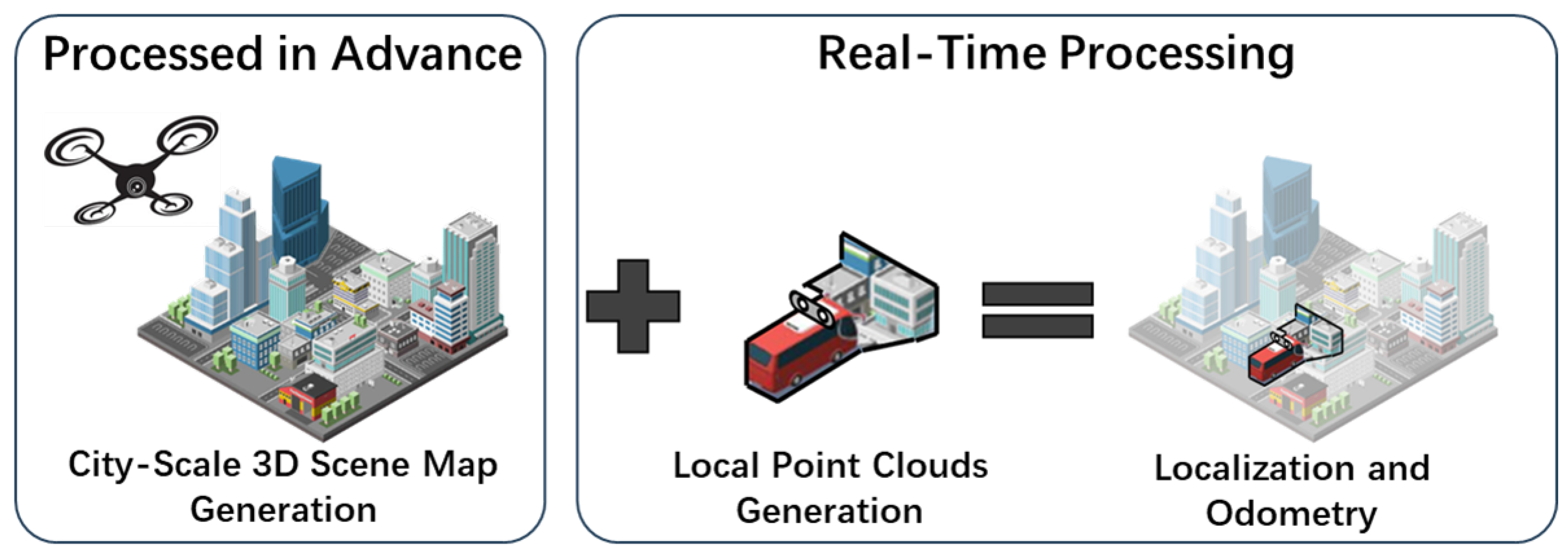
• A novel vehicle localization system is proposed by integrating aerial and ground views. The system enables vehicle localization and odometry while reconstructing the 3D large scene model.
• A building completion algorithm based on a geometric structure that significantly enhances the accuracy of UAV large-scene reconstruction is proposed. The algorithm also helps establish a 3D geometric relationship from the aerial view to the ground view, integrating 3D information from both perspectives.
• Experiments were performed using a dataset generated from the CG simulator to simulate the real scene. The results demonstrate the effectiveness of the proposed vehicle localization system in fusing aerial and ground views.

2. Related Work

This work mainly investigates the impact of city-scale 3D models reconstructed by UAVs on vehicle localization. The related work primarily falls into three parts: 3D reconstruction with UAVs, priori map-based SLAM, and aerial-to-ground SLAM.

2.1. Three-Dimensional Reconstruction with UAVs

Reconstructing a 3D large scene model using UAVs is the most efficient method in 3D urban modeling. Numerous approaches have been proposed to address 3D city map reconstruction challenges. Bashar et al. proposed 3D city modeling based on Ultra High Definition (UHD) video [10], using UHD video acquired from UAVs for 3D reconstruction and comparing the reconstructed point cloud density with HD video results. While UHD video improves point cloud quality, the orthoscopic view from UAVs causes some information loss due to the occlusion problem with 2D figures. In 2021, Chen et al. proposed a 3D reconstruction system for large scenes using multiple UAVs, optimizing the trajectory drift problem in multi-drone tracking [11]. Increasing the number of captured images can partially reduce missing information resulting from occlusion issues. However, high-precision 3D map reconstruction with multiple UAVs entails increased labor and time costs during operation. Omid et al. employed UAV radio measurements for 3D city reconstruction [12]. Although radio measurements provide higher ground reconstruction accuracy than visual sensors, they cannot avoid missing information due to occlusions such as building roofs in aerial views. Furthermore, the reconstructed model lacks RGB information, which is unfavorable for the potential rendering or visualization of the 3D city model. In 2022, Huang et al. employed the topological structure of building rooftops to complete the missing wall surfaces in drone-based 3D reconstruction [13]. However, this approach utilized a higher-precision radar for reconstruction and incorporated both interior and exterior wall information during the completion process. For vehicles, the interior wall surfaces of buildings act as noise and can cause drift in the localization process. In our system, a point cloud completion algorithm based on architectural geometry is proposed to address the issue of missing building walls caused by occlusion in the drone’s frontal view. This method selectively preserves only the exterior wall information, which is more relevant to the building, while retaining the RGB information from the visual sensor. Simultaneously, it resolves potential occlusion problems.

2.2. Priori Map-Based SLAM

SLAM is a widely used technology in vehicle localization and mapping. Applying SLAM to large scenes involves calculating the relative pose relationship between the camera coordinate system, the world coordinate system, and the image coordinate system. Most traditional visual SLAMs match feature points in each image frame to track the camera, only establishing the pose relationship between frames but not localizing the camera coordinates in large scenes. Research on pose optimization in SLAM using prior information generally relies on in-vehicle sensors [14,15] or high-precision maps [16]. On the one hand, in-vehicle sensors only provide perspective information limited to the area surrounding the vehicle (e.g., roads or bridges) [17], which is hard to obtain the whole city map. During the mapping process, moving on the road for map creation also carries significant restrictions in terms of freedom to compare with the UAV movements. Furthermore, to ensure that the features of the prior map can match the features obtained during the localization process, the same sensor is generally used for mapping and localization. This imposes many restrictions specific to the sensor for the SLAM system. On the other hand, creating high-precision maps for city-scale models is quite expensive as they require costly equipment, such as Light Detection and Ranging (LiDAR), and sometimes manual repairs are needed [18]. In this work, a method is proposed for assisting vehicle positioning by obtaining low-precision prior large scene maps using inexpensive drones. Our method uses drones with higher degrees of freedom to obtain prior maps and achieves a localization accuracy close to that of using high-precision maps while complementing the city model reconstructed by the UAVs. This work addresses the cost challenges related to high-precision map creation and also expands the possibilities for using 3D prior maps for localization.

2.3. Aerial-to-Ground SLAM

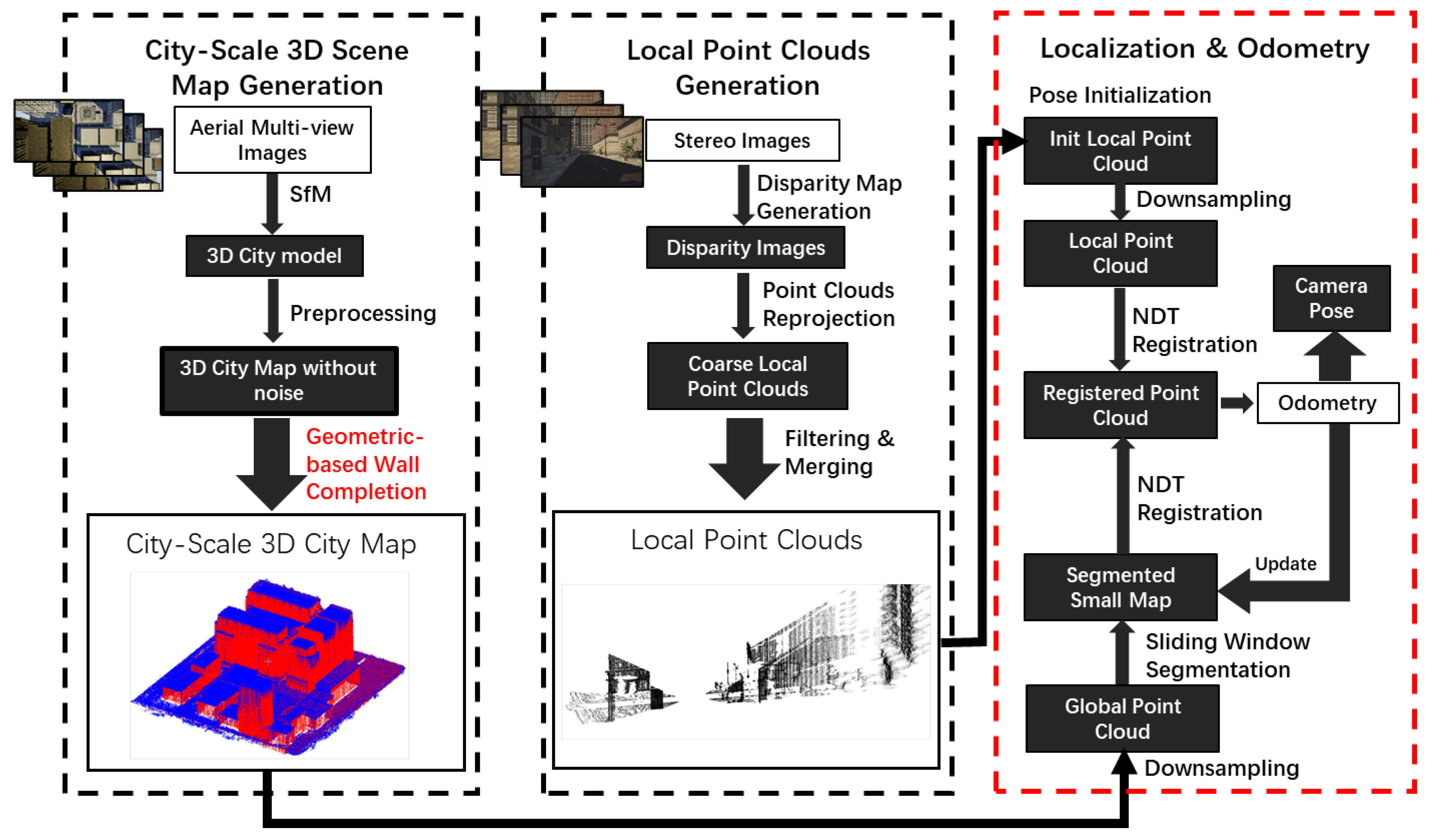
Substantial works are related to utilizing aerial perspectives to aid in ground-based positioning. For instance, Kummerle et al. [19] achieved impressive results by assisting radar-based positioning with global information from aerial images. In 2022, Shi et al. [20] used satellite images to assist in ground-based vehicle localization, helping the vehicles acquire accurate global information. These methods involve extracting features from 2D aerial images and matching them with ground-based information. Compared to 2D images, the feature set from 3D information obtained after urban reconstruction is more abundant. However, due to the immense volume of 3D information, its use in assisting localization can impact the real-time performance of the system. Moreover, there is a significant discrepancy between the 3D information computed from aerial data and that from ground data, making the match between the aerial and ground perspectives even more challenging to achieve. This paper proposes a method that uses the 3D information from drone reconstruction to assist in vehicle localization. Furthermore, by segmenting the global point cloud map, the data volume for vehicle localization is reduced to ensure the system’s real-time performance.

3. System Overview

The system consists of three main parts: city-scale 3D scene reconstruction, local point cloud generation from the onboard camera, and localization of the onboard camera within the large scene. Figure 2 illustrates the structure of the entire system. Initially, a UAV is utilized to capture aerial multi-view images and roughly reconstruct the city-scale 3D scene into a point cloud using the Structure from Motion (SfM) method [21]. After preprocessing the city-scale 3D scene, a point cloud model is obtained with reduced noise and real-world dimensions. Then the missing building walls in the large scene are completed by extracting the building’s geometric features in a layer-wise manner. The point cloud of the completed large-scene points serves as a prior map for optimizing the onboard camera’s pose.

In the local point cloud generation session, stereo images captured from two pairs of onboard cameras from the front and rear of the vehicle are utilized. Then the disparity maps and matching the depth information pixel by pixel to the RGB data are calculated to generate a dense local point cloud. This process is repeated frame by frame. In one frame processing, the front point cloud with the back point cloud is merged and filtered out noise in the point cloud using outlier removal.

In the localization and odometry sessions, both local and global point clouds are downsampled to ensure their densities are almost the same, which leads to more accurate registration. To accelerate the matching process and reduce computational effort, a sliding window algorithm is employed to segment the global point cloud based on the vehicle’s current position. For localization and alignment, the normal distributions transform (NDT) point cloud registration [22] algorithm is used to calculate and update the rotation and translation matrices from the vehicle coordinates system to the world coordinates system in real-time so that the vehicle in the global map can be located. The relevant algorithms are introduced involved in each of the three sections below.

4. City-Scale 3D Scene Map Generation

4.1. Structure from Motion

The Structure from Motion (SfM) method [21] is a common approach for constructing 3D structures from multi-view aerial images. SfM follows a sequential pipeline with an iterative reconstruction component, wherein selecting the optimal initial image pair to seed the reconstruction represents a crucial step. After geometric verification through feature extraction and matching, the initialized image pair undergoes iteration. By progressively incorporating new images, SfM can register them with the initial images to optimize the reconstructed scene points and the estimated camera pose. Through step-by-step bundle adjustment, the extrinsic parameters of the camera can be computed, and the scene geometry information can be obtained as a 3D point cloud.

To enhance the 3D model of the large scene, the sparse 3D point cloud is optimized through dense point cloud reconstruction. Nevertheless, the reconstructed model can be affected by noise and scale issues, necessitating preprocessing of the 3D scene model. This work includes outlier removal to eliminate noisy points that might arise from feature point mismatches. As SfM reconstruction is not scale-invariant, rescaling the large scene to the real-world scale is necessary. To achieve this, markers are set, and the difference between markers in the ground truth and the SfM model is computed to determine the scale ratios. The whole process of SfM is all developed on the Pix4D Mapper V4.7.

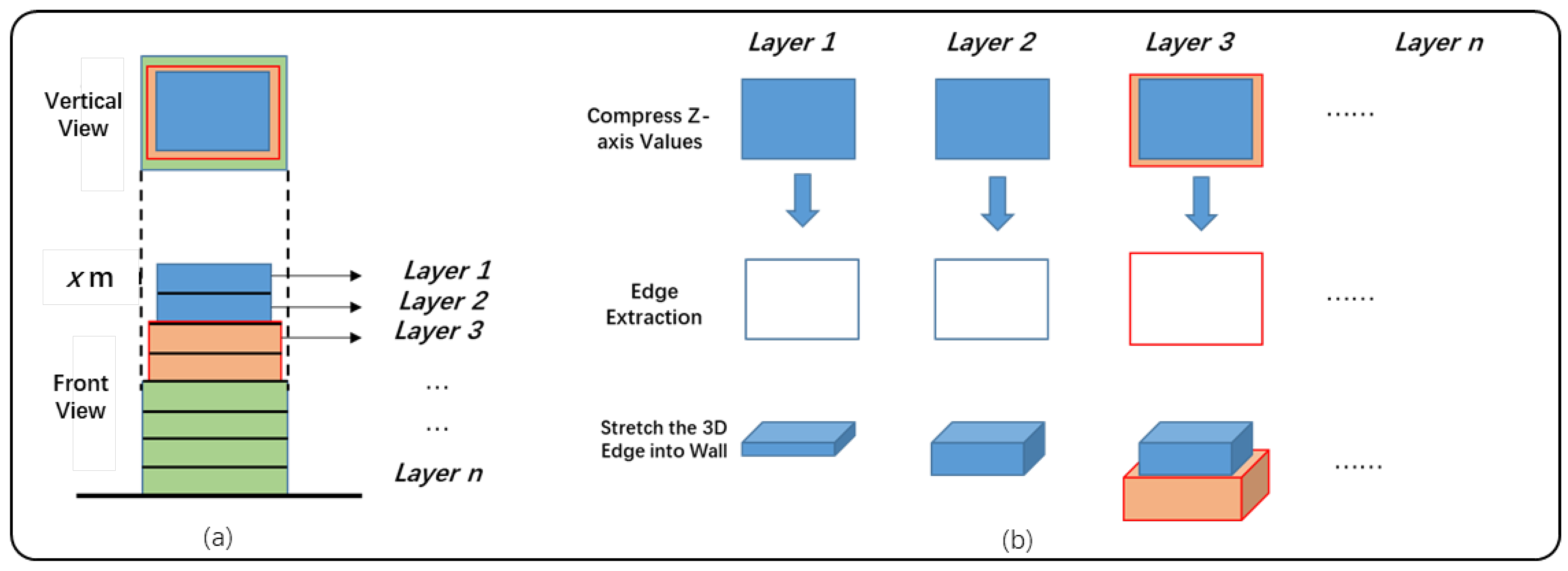
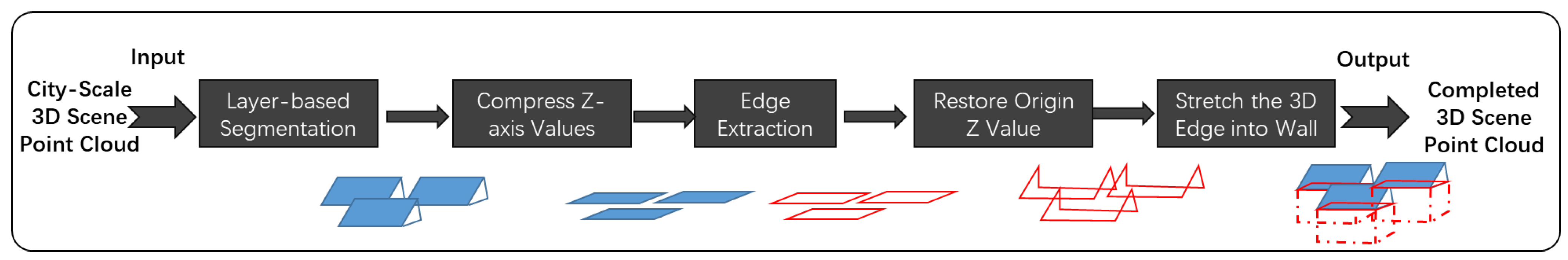
4.2. Geometry-Based Wall Completion

After the preprocessing of noise canceling and scaling, an incomplete 3D scene model with fewer noisy points is obtained. However, due to the occlusion of roofs and other building structures, the 3D scene model lacks wall information which is crucial for localization. Identifying shared information to correct registration is a critical problem that needs to be addressed to fuse UAV views with ground views. Only with shared features can we calculate the relative pose relationship from the camera coordinates of the onboard camera to the UAV’s camera. When generating a large scene map using the ortho-view of the UAV, most information primarily focuses on building roofs. However, the roof point cloud cannot be obtained from the ground view. The point cloud obtained from the onboard cameras mainly consists of building walls and roads. Therefore, to build the shared feature, a novel algorithm is proposed to generate the wall point cloud from UAV views based on the geometric features of the building. The specific completion process is described in detail below.

4.2.1. Layer-Based Segmentation

This section introduces a layer-based point cloud segmentation method based on architectural geometry. The method effectively helps extract the geometric features of the top layer of a building to complement the wall structure of the lower layers, thus improving the accuracy and completeness of the 3D scene model.

According to conventional architectural geometry, the walls of a building may be approximated by extending the edges of the eaves. However, since most building structures are similar to pyramid constructions, the area near the ground is greater than the area at the top. The walls stretched only by the roof information is inaccurate near the ground. Therefore, the 3D city model is divided into different layers based on height from top to bottom (z-axis) and inherits the geometric features of the building’s top layer to the wall structure of the lower layers through top-down processing. As shown in Figure 3a, the building is divided into layers with a height of x meters, and the wall edge information extracted from layer $h_i$ will be used in the wall stretching process of the layer below $h_{i-1}$. As shown in Figure 3b, by judging whether the overall area of layer $h_{i-1}$ is greater than the area of layer $h_i$, we can then determine if it is accurate wall edge information before performing the wall stretching algorithm. The choice of layer height is flexible but should be smaller than the height of each floor in the real world, as the difference in area between the upper and lower layers is mainly reflected in the change of floors. However, the smaller the layer height, the more layers will be divided, which will lead to increased computation costs.

4.2.2. Wall Completion Algorithm

A wall completion algorithm based on building wall edge detection is proposed. The detailed process and the generated models at each step are shown in Figure 4. The specific algorithm workflow is as follows: First, the point cloud using the layer-based segmentation described before is segmented. The point cloud of each layer is then compressed to a 2D plane by removing the z-axis (height). It can be observed that the edges of each point cloud cluster represent 2D eaves, thereby can be stretched along the z-axis to reconstruct building walls. The edge extraction of the point cloud clusters is based on the angle criterion point cloud edge detection method. The algorithm on a 2D scale is utilized, and the definition of the edge points can be shown in Figure 5. Finally, the wall surfaces of the entire map are completed, which is shown in Figure 6. By employing this layered point cloud completion method based on architectural geometry, the system can achieve more accurate wall structures in the 3D scene model.

5. Local Point Cloud Generation

5.1. Disparity Map Generation

A stereo camera is used to generate the local point cloud from the vehicle. Binocular stereo vision is based on disparity, and the disparity map is calculated using the semi-global block matching (SGBM) method [23]. SGBM takes into account a larger context by aggregating costs along multiple paths throughout the image, which leads to more reliable disparity estimates, particularly near-depth discontinuities, and occlusions, without the high computational cost of fully global methods. However, the output of SGBM has noise at the contour of the object. Typically, a smoothness algorithm is necessary for noise removal. In this work, the weighted least squares (WLS) filter [24] is used, an edge-preserving smoothing filter, to smooth the disparity map.

5.2. Point Cloud Reprojection

To generate the local point cloud, the depth value from the image plane is needed to reproject to the 3D world. The 3D information is acquired by the principle of trigonometry, which is formed between the image plane of the two cameras and the measured points. By using the intrinsic parameters and extrinsic parameters of two cameras, the coordinate of the local point cloud $P(x,y,z)$ can be computed as follows:

$$\left\{\begin{array}{cc}x={\displaystyle \frac{B·X_{left}}{disparity}},\hfill & \\ y={\displaystyle \frac{B·Y_{left}}{disparity}},\hfill & \\ z={\displaystyle \frac{B·f}{disparity}},\hfill \end{array}\right.$$

(1)

B is for the baseline of the stereo camera. $X_{left}$ and $Y_{left}$ are the pixel values of the left image in the image plane coordinate system. Using Equation (1), the 2D points are able to be reprojected into 3D point clouds. Figure 7 shows an example of the generated disparity map and the reprojected 3D point cloud.

5.3. Filtering and Merging

During the localization process, the local point cloud of each frame is acquired in real-time for matching with the city-scale point cloud. An outlier removal algorithm is applied to reduce the noise of the acquired local point clouds [25]. It is noteworthy that depth measurement by stereo vision becomes less precise with increasing distance due to the nature of triangulation [26]. Therefore, to reduce the effect of long-range point cloud noise on matching results, the point cloud within a radius of 50 m from the vehicle is used for localization. The chosen distance is deemed appropriate, given the baseline size of the stereo camera and the measurable distance of the majority of vehicle sensors in practical scenarios. Having the extrinsic parameters of both front and rear stereo cameras, the front and rear point clouds can be merged into one local point cloud. The output point cloud is shown in Figure 8.

6. Localization and Odometry

6.1. Downsampling

Owing to the distinct acquisition methods employed for local and global point clouds, the resulting point clouds can exhibit substantial disparities in density. Primarily, this occurs because the local point cloud constitutes a dense cloud projected by the onboard camera based on each pixel, whereas the global city-scale point cloud comprises a sparse cloud obtained by the UAV through feature point estimation and point cloud completion. To attain precise camera poses, it is essential to minimize the density differences between the two point clouds. Consequently, downsampling both point clouds is a critical step in this process. In this work, voxel downsampling is used to ensure that the point cloud densities are analogous. Voxel downsampling is executed by defining a specific density of voxels and subsequently retaining a random point within the voxel. This approach preserves the majority of the geometric information contained in the point cloud while also enabling the unification of two point clouds to nearly identical densities.

6.2. Sliding Window Segmentation

Given the large data size of extensive scene maps, matching them with local maps through each frame demands significant computational power and may easily yield locally optimal solutions. This work refers to the sliding window segmentation in the radar global localization algorithm [27] to segment the large scene map into a small scene map according to the moving position of the vehicle. When the vehicle is detected to have exited the small scene map, the large scene map is re-segmented into a new smaller scene piece. Due to the reduced amount of data, the segmentation approach can significantly reduce computational complexity.

For segmentation, the CropBox method in the Point Cloud Lab (PCL) is employed. This technique fundamentally involves segmenting a small point cloud from a larger point cloud based on the dimensions of a bounding box. The size of the bounding box is determined according to the measurable range of the onboard camera. The bounding box center’s coordinate in the global map corresponds to the vehicle pose in the current frame. In this study, we set up that if the distance between the edge of the bounding box and the current vehicle pose is less than 50 m, the smaller scene map is re-segmented with the current position as the origin. The re-segmented smaller scene map is then used for the subsequent registration step with the local point cloud map, optimizing the cumulative error of the onboard camera.

6.3. Pose Initialization

Because we need to know the initial position in order to segment the large scene map and localize the vehicle next, pose initialization is necessary. The coordinate system employed in the entire system encompasses the world coordinate system, the vehicle’s local coordinate system, and the Earth coordinate system. As shown in Figure 9, the world coordinate system represents the coordinate of the large scene point clouds, while the local coordinate system moves with the vehicle camera as the origin. The Earth coordinate system signifies the coordinate relationship between the GPS sensor and the Earth. During the SLAM simulation, the world coordinate system is defined according to the Earth coordinate system to facilitate easier acquisition of GPS information. Because the vehicle and the GPS sensor share the same position, the GPS information is utilized to initialize the vehicle’s local coordinate system and locate it within the world coordinate system.

6.4. NDT Registration

To register two point clouds, NDT registration [22] is applied to calculate the rigid transformation matrix R and T. The calculation of the inter-frame local point cloud transformation and the local point cloud to small scene point cloud alignment optimization are all based on this method. The specific calculation method is to divide the two point clouds into cells and calculate the mean and covariance matrix of the points contained in each cell. As a result, the normal distribution of points in a cell can be expressed by $p\left(x\right)$ as:

$$p\left(x\right)\approx exp\left({\displaystyle \frac{{(x_i-q)}^t{\sum }_i^{-1}(x_i-q)}{2}}\right)$$

where $x_i$ denotes the position of the ith point in the cell $(x_i,y_i,z_i)$, q denotes the mean value of the contained points. ∑ is the covariance matrix. The score of NDT alignment is defined by the sum of the probabilities of the corresponding points in the corresponding cell after transformation:

$$score\left(p\right)=\sum _{i}exp\left({\displaystyle \frac{{({x^{\prime }}_i-q_i)}^t{\sum }_i^{-1}({x^{\prime }}_i-q_i)}{2}}\right)$$

The transformation matrix R, T is optimized by maximizing the score using Gauss-Newtons method [28].

In point cloud registration, it has been observed from the formula that NDT presents distinct advantages over traditional algorithms, such as Iterative Closest Point (ICP) [29]. One of the most prominent benefits lies in the utilization of probability density functions in NDT’s computational process. This innovative approach considerably simplifies calculations, which, in turn, reduces the computational burden in the point cloud registration process. The whole system is designed to operate in real time, which requires the computation of exceptionally large point clouds. Thus, the efficiency of the registration process is paramount to ensure system performance. Given these constraints, opting for the NDT methodology over traditional ICP registration offers a significant boost in the real-time responsiveness of the system.

7. Experiment and Results

To evaluate the effectiveness of the algorithm, Unreal Engine (UE) 4 is used to simulate real-world situations, which is a 400 m × 400 m shopping district scene, including typical street scenes such as streets, buildings, traffic signs, and trees. Light is also rendered to make the scene realistic. The whole scene is shown in Figure 10. Then, the UAVs and vehicles are simulated in the UE4 to record the dataset with both UAV views and the ground view.

7.1. Point Cloud Completion

The UAVs are simulated using Microsoft AirSim [30]. An RGB camera with a resolution of 2704 pixels × 1520 pixels is mounted on the bottom of the UAV. To acquire orthorectified multi-view aerial images, the UAV is set at an altitude of 120 m and moved in a grid-like pattern to acquire images, as shown in Figure 11. The height of 120 m is determined because the maximum flight height of UAVs allowed by Japanese aviation law is 150 m, so a typical height chosen is slightly less than 150 m. To obtain the ground truth for the large scene model, the 3D model of the whole scene is exported, and the model is uniformly sampled into a point cloud.

To test the effectiveness of the wall completion algorithm, point clouds of a large 3D scene were compared before and after the use of the wall completion algorithm. Both the completeness of the point cloud reconstruction and the accuracy of the completion were evaluated. The point-to-point distance was calculated as the distance between the ground-truth point cloud and the large scene point cloud. Firstly, the Iterative Closest Point (ICP) [31] registration method is employed to effectively align two point clouds. Following the alignment, the Octree method was utilized to efficiently identify the nearest points between the two point clouds. The point-to-point distance, defined as the absolute Euclidean distance between corresponding query points, serves as a crucial metric for assessing both the reconstruction completeness and accuracy. The point-to-point distance enables a comprehensive evaluation of the quality and precision of the reconstructed point clouds, ensuring reliable and robust results in various applications. A larger point-to-point distance means a larger error between the point clouds. Errors mainly come from the fact that vision-based 3D reconstruction produces a portion of feature-matching errors when performing BA, as well as missing point clouds due to occlusion. In this work, only the missing points are discussed but not the error from the SfM method. CloudCompare software was used to register the completed point cloud with the ground-truth point cloud and calculate the distance between the points to evaluate accuracy. The result is shown in Figure 12. It can be seen that there is a significant improvement in the points with an error range of 5 m or less before and after completion. The points completed in accordance with the shape of the building are reliable.

In addition, Figure 13 shows a heat map of the absolute distance between points created to represent the completeness of the restored point cloud. In this case, the distance between points is displayed as a gradient from red to blue, from larger to smaller. The smaller the distance, the more the heat map is colored blue. It can be seen that the absolute distance is very large in the reconstructed model, especially in the area of walls because there is no point cloud. The absolute distance in the building wall area is much smaller after completion, indicating that the completion algorithm has improved the consistency of the 3D reconstruction of a large scene.

An experiment is set up to validate the effectiveness of layer-based completion on the city models. Different heights of segmented layers (5 m, 10 m, 30 m, 60 m) are set up to complete the large scene model. Furthermore, the point-to-point distances are compared between the completed city model and the ground truth. To present the accuracy more effectively, a Gaussian curve is fitted to the distance histogram, and the mean and standard deviation of the curve are calculated, which is shown in Figure 14 The results of the experiment indicate that the smaller the layer size used for segmentation, the closer the completed urban model aligns with the ground truth model. This observation suggests that hierarchical completion is more effective in producing accurate urban models when the layers are divided into smaller subunits. This is mainly because denser segmentation of layers allows for a higher concentration of features during the wall stretching process, preserving the layer-specific information. Since the completion in each layer relies on the edge information of the city model from the layer above, the walls completed within the same layer are identical. By employing denser layer segmentation, the urban model retains a greater amount of diverse height information, leading to the preservation of more crucial details. Consequently, the completion results are more accurate and favorable.

7.2. Localization and Odometry

To compare the estimated vehicle trajectory and the actual vehicle trajectory, the motion of the vehicle is simulated in the CG simulator as the large scene. The vehicle model is simulated by Microsoft AirSim and moves along different routes on the road. Two pairs of RGB cameras with a resolution of 2704 pixels × 1520 pixels are placed at the front and rear of the vehicle to simulate the ground view capture. The baseline of the cameras is set to 540 mm to measure long-distance depth. During the simulation, the vehicle is manually manipulated, and the sensor information is recorded at 30 frames per second. GPS and IMU sensors are also installed on the vehicle to capture the 6 degrees of freedom pose of the onboard camera with a Gauss noise in 0.2 ratios. The pose is only used for initialization but not the whole odometry process. The ground truth of the vehicle trajectory is obtained by recording the vehicle coordinates in the world coordinate system.

We evaluate the accuracy of the algorithm by designing an L-shaped route, a U-shape route, and a Z-shape route. The reason for choosing different forms of routes is to test the robustness of the algorithm under different route scenarios. The starting positions of the routes are set at different locations in the city, and the routes are all designed to ensure that they pass through different streets in the city model. Figure 15 shows the routes in the city map seen from the top view.

During the experiment, the localization results are compared by using the original large scene model, completed large scene model, and high-precision large scene model as the global map prior. The high-precision city model is set up by using the ground truth of the city model.

We plotted the trajectory maps based on the estimated vehicle poses for different routes and different prior conditions, as shown in Figure 16. It can be seen that the higher accuracy of the large scene model makes the vehicle odometry more accurate. Since some wall information is missing in the original map, this prevents the vehicle from matching information such as wall corners that are useful for determining the distance of the vehicle movements. It is also difficult to obtain feature information such as walls that are favorable for judging the constrained left and right displacements of the vehicle. Therefore, when using the original map for localization, the exact pose of the vehicle cannot be obtained. This result highlights the importance of shared features in 3D point cloud feature matching. However, the optimized localization using the point cloud completion algorithm is almost similar to the localization accuracy using the ground truth city model. This is because most of the localization information for the ground view of the vehicle comes from geometric features that provide longitudinal depth from aerial to the ground. In contrast, the UAVs cannot provide enough longitudinal information due to the orthorectified view factor, which affects the localization of the ground view. In addition, we can also find that there are some drift errors at the corners, which are due to the occlusion on the corner. The occlusion makes the point cloud generation not accurate enough, leading to the mismatching between the local point cloud and the large scene model. However, the localization can be repaired when the ground view can obtain enough features for matching.

The trajectory is evaluated using two metrics: absolute trajectory error (ATE) and relative pose error (RPE). ATE is the metric that calculates the difference between the estimated trajectory and ground truth. It is used to investigate the global consistency of a SLAM trajectory. RPE is the metric that calculates the difference in pose change over the same time stamp. It is used to investigate the local consistency of a SLAM trajectory.

Table 1. The ATE of using different prior maps as input. Origin represents using the original uncompleted large scene map as input. Completed represents using the completed large scene map as input. High-Precision represents using the high-precision large scene map as input. (Units: m).

	Origin				Completed				High-Precision
	RMSE	MEAN	Median	S.D.	RMSE	MEAN	Median	S.D.	RMSE	MEAN	Median	S.D.
L_route	40.571	34.692	35.285	20.930	11.672	9.331	6.956	7.012	5.377	4.457	3.351	3.010
Z_route	28.978	24.253	19.337	15.860	3.909	3.538	3.353	1.663	3.268	2.629	1.937	1.441
U_route	28.864	26.373	25.384	11.843	5.634	4.980	4.828	2.635	4.929	4.383	4.124	2.257

and

Table 2. The RPE of using different prior maps as input. Origin represents using the original uncompleted large scene map as input. Completed represents using the completed large scene map as input. High-Precision represents using the high-precision large scene map as input. (Units: m).

	Origin				Completed				High-Precision
	RMSE	MEAN	Median	S.D.	RMSE	MEAN	Median	S.D.	RMSE	MEAN	Median	S.D.
L_route	6.339	4.964	3.864	3.943	1.689	1.108	0.895	1.275	1.272	0.939	0.760	0.858
Z_route	2.764	2.258	2.087	1.594	1.413	1.087	0.790	0.903	0.826	0.593	0.292	0.576
U_route	4.671	3.874	3.747	2.609	1.763	1.263	1.008	1.230	1.561	1.231	0.969	0.960

show the results of different routes with different prior conditions.

For further comparison, root mean square error (RMSE), mean value, median value, and standard deviation (S.D.) are compared in Table 1 and Table 2. Since RMSE is more sensitive to large or occasional errors [32], it can be used to evaluate the robustness of the system. Mean and Median are used to evaluate the average error of the whole system. S.D. is used to evaluate the stability of the system [33]. The errors of using the complemented large scene point cloud map and the high-precision model in our system are close and much smaller than that of directly using the original point cloud reconstructed by UAVs for localization. The results verify that our localization system remains robust under different routes.

In addition, the method in this work is compared with the state-of-the-art approaches. As our method is based on 3D point cloud registration, it is better suited for the A-LOAM [34] localization framework. The A-LOAM framework estimates vehicle poses by optimizing the matching between consecutive 3D point clouds without relying on prior maps. The experiments were conducted on three different paths: L-shaped, U-shaped, and Z-shaped. The estimated pose results are shown in Figure 17. By calculating the ATE and RPE, we obtained the results presented in

Table 3. The ATE of using A-LOAM and this work. A-LOAM represents using the A-LOAM framework for frame-to-frame registration. Completed represents using the completed large scene map as input. (Units: m).

	A-LOAM				Completed
	RMSE	MEAN	Median	S.D.	RMSE	MEAN	Median	S.D.
L_route	12.441	10.402	9.647	7.823	11.672	9.331	6.956	7.012
Z_route	9.226	7.510	6.042	5.359	3.909	3.538	3.353	1.663
U_route	13.325	12.075	10.407	5.636	5.634	4.980	4.828	2.635

and

Table 4. The RPE of using A-LOAM and this work. A-LOAM represents using the A-LOAM framework for frame-to-frame registration. Completed represents using the completed large scene map as input. (Units: m).

	A-LOAM				Completed
	RMSE	MEAN	Median	S.D.	RMSE	MEAN	Median	S.D.
L_route	3.943	2.741	2.552	1.590	1.689	1.108	0.895	1.275
Z_route	2.841	2.350	2.213	1.394	1.413	1.087	0.790	0.903
U_route	4.263	4.011	4.817	1.824	1.763	1.263	1.008	1.230

.

The results demonstrate that our approach achieved superior localization performance. Since the 3D point clouds acquired by the stereo camera are inherently prone to inaccuracies, errors are introduced during the matching process between consecutive frames. Accumulation of these errors can result in significant scale and matching inaccuracies in the localization. However, employing a prior map helps to mitigate the issue of misalignment caused by inaccuracies in the stereo camera’s point cloud estimation. Each frame is corrected during the matching process with the prior map, leading to a substantial reduction in scale errors.

Furthermore, it was observed that in U-shaped paths, the estimation of poses tends to be more error-prone, particularly at the turning points. This is primarily attributed to the larger angular changes in consecutive point clouds when the vehicle makes sharp turns at high speeds, making it challenging to establish accurate frame-to-frame matching. Moreover, once the vehicle completes a turn without reference objects, the current pose cannot be effectively corrected. However, when utilizing the prior map for aiding navigation, this issue of misalignment caused by significant turning errors can be effectively rectified. The vehicle automatically corrects its localization using the prior map during subsequent operations.

Overall, the experimental results demonstrate the effectiveness of our proposed method in achieving improved localization accuracy, particularly in scenarios where stereo camera-derived point clouds may lead to matching errors. The integration of a prior map in the work significantly enhances the robustness of the localization process, particularly in challenging urban environments with complex and dynamic surroundings.

8. Conclusions

In this paper, a large scene SLAM algorithm is proposed by combining aerial view and vehicle-mounted stereo cameras. The large scene 3D reconstruction based on the aerial view is optimized using point cloud complementation based on geometric features. The vehicle is localized using the vehicle-mounted stereo camera by employing 3D point pair matching. The proposed SLAM algorithm unifies the aerial view and ground view and solves the problem of an inability to match due to the absence of common features in different views. A CG simulator is used to acquire the dataset and simulate the system. The results showed that the proposed point cloud complementation algorithm could effectively complement the wall information of the 3D large scene model, and the wall information could be utilized for vehicle localization in the large scene.

9. Discussion

Our method still has some limitations. Firstly, in the city-scale scene 3D reconstruction completion algorithm, our approach leverages the geometric features of rooftops and layer-based edge extraction to perform top-down wall completion. Consequently, it is only applicable to pyramid-type structures with smaller top areas and larger base areas. For complex structures in urban environments, it is still difficult for our method to reconstruct the buildings accurately, potentially affecting the precision of city-scale scene 3D reconstruction. Secondly, our method relies on accurate 3D feature matching. The localization accuracy mainly depends on the similarity of the point clouds acquired from different viewpoints. When there is a large error between the complemented point cloud and the point cloud of the ground view, it may lead to matching failure. In our analysis, due to the lack of accessible open-source datasets, we employed a CG simulator to simulate experimental data. Our objective was to emulate driving environments to the best of our abilities, but real-world scenarios often present more intricate factors, such as uneven road surfaces, which can impact actual positioning accuracy. Moving forward, we intend to gather data from real-world settings and explore algorithmic improvements to address the issues that arise in practical contexts. In future work, the sensitivity and accuracy of our method need to be improved to make the algorithm more robust in dealing with different environments and occlusion problems.

References

1. Ibragimov, I.Z.; Afanasyev, I.M. Comparison of ROS-based visual SLAM methods in homogeneous indoor environment. In Proceedings of the 2017 14th Workshop on Positioning, Navigation and Communications (WPNC), Bremen, Germany, 25–26 October 2017; pp. 1–6. [Google Scholar] [CrossRef]
2. Blochliger, F.; Fehr, M.; Dymczyk, M.; Schneider, T.; Siegwart, R. Topomap: Topological Mapping and Navigation Based on Visual SLAM Maps. In Proceedings of the 2018 IEEE International Conference on Robotics and Automation (ICRA), Brisbane, QLD, Australia, 21–25 May 2018; pp. 3818–3825. [Google Scholar] [CrossRef] [Green Version]
3. Mur-Artal, R.; Montiel, J.M.M.; Tardos, J.D. ORB-SLAM: A versatile and accurate monocular SLAM system. IEEE Trans. Robot. 2015, 31, 1147–1163. [Google Scholar] [CrossRef] [Green Version]
4. Shan, T.; Englot, B. Lego-loam: Lightweight and ground-optimized lidar odometry and mapping on variable terrain. In Proceedings of the 2018 IEEE/RSJ International Conference on Intelligent Robots and Systems (IROS), Madrid, Spain, 1–5 October 2018; IEEE: Pisctaway, NJ, USA, 2018; pp. 4758–4765. [Google Scholar]
5. Zhao, S.; Zhang, H.; Wang, P.; Nogueira, L.; Scherer, S. Super odometry: IMU-centric LiDAR-visual-inertial estimator for challenging environments. In Proceedings of the 2021 IEEE/RSJ International Conference on Intelligent Robots and Systems (IROS), Prague, Czech Republic, 27 September–1 October 2021; IEEE: Pisctaway, NJ, USA, 2021; pp. 8729–8736. [Google Scholar]
6. Cui, L.; Wen, F. A monocular ORB-SLAM in dynamic environments. J. Phys. Conf. Ser. 2019, 1168, 052037. [Google Scholar] [CrossRef]
7. Wang, Q.; Zhang, J.; Liu, Y.; Zhang, X. High-Precision and Fast LiDAR Odometry and Mapping Algorithm. J. Adv. Comput. Intell. Intell. Inform. 2022, 26, 206–216. [Google Scholar] [CrossRef]
8. Liu, R.; Wang, J.; Zhang, B. High definition map for automated driving: Overview and analysis. J. Navig. 2020, 73, 324–341. [Google Scholar] [CrossRef]
9. Fruh, C.; Zakhor, A. Constructing 3D city models by merging aerial and ground views. IEEE Comput. Graph. Appl. 2003, 23, 52–61. [Google Scholar] [CrossRef] [Green Version]
10. Alsadik, B.; Khalaf, Y.H. Potential Use of Drone Ultra-High-Definition Videos for Detailed 3D City Modeling. ISPRS Int. J. Geo-Inf. 2022, 11, 34. [Google Scholar] [CrossRef]
11. Chen, F.; Lu, Y.; Cai, B.; Xie, X. Multi-Drone Collaborative Trajectory Optimization for Large-Scale Aerial 3D Scanning. In Proceedings of the 2021 IEEE International Symposium on Mixed and Augmented Reality Adjunct (ISMAR-Adjunct), Bari, Italy, 4–8 October 2021; pp. 121–126. [Google Scholar] [CrossRef]
12. Esrafilian, O.; Gesbert, D. 3D city map reconstruction from UAV-based radio measurements. In Proceedings of the GLOBECOM 2017—2017 IEEE Global Communications Conference, Singapore, 4–8 December 2017; IEEE: Piscatway, NJ, USA, 2017; pp. 1–6. [Google Scholar]
13. Huang, J.; Stoter, J.; Peters, R.; Nan, L. City3D: Large-scale building reconstruction from airborne LiDAR point clouds. Remote Sens. 2022, 14, 2254. [Google Scholar] [CrossRef]
14. Sasiadek, J.Z.; Ahmed, A. Multi-Sensor Fusion for Navigation of Ground Vehicles. In Proceedings of the 2022 26th International Conference on Methods and Models in Automation and Robotics (MMAR), Międzyzdroje, Poland, 22–25 August 2022; pp. 128–133. [Google Scholar] [CrossRef]
15. Liu, Y.; Yang, D.; Li, J.; Gu, Y.; Pi, J.; Zhang, X. Stereo Visual-Inertial SLAM with Points and Lines. IEEE Access 2018, 6, 69381–69392. [Google Scholar] [CrossRef]
16. Liu, J.; Xiao, J.; Cao, H.; Deng, J. The Status and Challenges of High Precision Map for Automated Driving. In Proceedings of the China Satellite Navigation Conference (CSNC), Beijing, China, 22–25 May 2019; Sun, J., Yang, C., Yang, Y., Eds.; Springer: Singapore, 2019; pp. 266–276. [Google Scholar]
17. Guizilini, V.; Ambrus, R.; Pillai, S.; Raventos, A.; Gaidon, A. 3D packing for self-supervised monocular depth estimation. In Proceedings of the IEEE/CVF Conference on Computer Vision and Pattern Recognition, Seattle, WA, USA, 13–19 June 2020; pp. 2485–2494. [Google Scholar]
18. Lin, L.; Liu, Y.; Hu, Y.; Yan, X.; Xie, K.; Huang, H. Capturing, Reconstructing, and Simulating: The UrbanScene3D Dataset. In Proceedings of the Computer Vision—ECCV 2022, Tel Aviv, Israel, 23–27 October 2022; Avidan, S., Brostow, G., Cissé, M., Farinella, G.M., Hassner, T., Eds.; Springer: Cham, Switzerland, 2022; pp. 93–109. [Google Scholar]
19. Kümmerle, R.; Steder, B.; Dornhege, C.; Kleiner, A.; Grisetti, G.; Burgard, W. Large scale graph-based SLAM using aerial images as prior information. Auton. Robot. 2009, 30, 25–39. [Google Scholar] [CrossRef] [Green Version]
20. Shi, Y.; Li, H. Beyond cross-view image retrieval: Highly accurate vehicle localization using satellite image. In Proceedings of the IEEE/CVF Conference on Computer Vision and Pattern Recognition, New Orleans, LA, USA, 18–24 June 2022; pp. 17010–17020. [Google Scholar]
21. Ullman, S. The Interpretation of Structure from Motion. Proc. R. Soc. Lond. Ser. B Biol. Sci. 1979, 203, 405–426. [Google Scholar]
22. Hong, H.; Lee, B.H. Probabilistic normal distributions transform representation for accurate 3D point cloud registration. In Proceedings of the 2017 IEEE/RSJ International Conference on Intelligent Robots and Systems (IROS), Vancouver, BC, Canada, 24–28 September 2017; pp. 3333–3338. [Google Scholar] [CrossRef]
23. Hirschmuller, H. Stereo Processing by Semiglobal Matching and Mutual Information. IEEE Trans. Pattern Anal. Mach. Intell. 2008, 30, 328–341. [Google Scholar] [CrossRef] [PubMed]
24. An, X.; Pellacini, F. AppProp: All-Pairs appearance-space edit propagation. ACM Trans. Graph. 2008, 27, 40. [Google Scholar] [CrossRef]
25. Balta, H.; Velagic, J.; Bosschaerts, W.; De Cubber, G.; Siciliano, B. Fast statistical outlier removal based method for large 3D point clouds of outdoor environments. IFAC-PapersOnLine 2018, 51, 348–353. [Google Scholar] [CrossRef]
26. Oh, J. Novel Approach to Epipolar Resampling of HRSI and Satellite Stereo Imagery-Based Georeferencing of Aerial Images. Ph.D. Thesis, The Ohio State University, Columbus, OH, USA, 22 July 2011. [Google Scholar]
27. Li, K.; Li, M.; Hanebeck, U.D. Towards High-Performance Solid-State-LiDAR-Inertial Odometry and Mapping. arXiv 2020, arXiv:2010.13150. [Google Scholar] [CrossRef]
28. Deuflhard, P. Newton Methods for Nonlinear Problems: Affine Invariance and Adaptive Algorithms; Springer Science & Business Media: Berlin/Heidelberg, Germany, 2005; Volume 35. [Google Scholar]
29. Zhang, Z. Iterative point matching for registration of free-form curves and surfaces. Int. J. Comput. Vis. 1994, 13, 119–152. [Google Scholar] [CrossRef]
30. Shah, S.; Dey, D.; Lovett, C.; Kapoor, A. AirSim: High-Fidelity Visual and Physical Simulation for Autonomous Vehicles. In Proceedings of the Field and Service Robotics, Zurich, Switzerland, 12–15 September 2017. [Google Scholar]
31. Zhang, Z. Iterative Closest Point (ICP). In Computer Vision: A Reference Guide; Ikeuchi, K., Ed.; Springer: Boston, MA, USA, 2014; pp. 433–434. [Google Scholar] [CrossRef]
32. Kerl, C.; Sturm, J.; Cremers, D. Robust odometry estimation for RGB-D cameras. In Proceedings of the 2013 IEEE International Conference on Robotics and Automation, Karlsruhe, Germany, 6–10 May 2013; pp. 3748–3754. [Google Scholar] [CrossRef] [Green Version]
33. Sun, Y.; Liu, M.; Meng, M.Q.H. Motion removal for reliable RGB-D SLAM in dynamic environments. Robot. Auton. Syst. 2018, 108, 115–128. [Google Scholar] [CrossRef]
34. Zhang, J.; Singh, S. LOAM: Lidar odometry and mapping in real-time. In Proceedings of the Robotics: Science and Systems, Berkeley, CA, USA, 12–16 June 2014; Volume 2, pp. 1–9. [Google Scholar]
Figure 1. A generic timeline of the entire process.
Remotesensing 15 03871 g001
Figure 2. The proposed algorithm framework involves generating a city-scale 3D city map in advance to create the global map. Local point clouds are generated in real time on the vehicle. Localization and odometry are used to match shared features between the global and local maps. The contribution of our work is highlighted in red.
Remotesensing 15 03871 g002
Figure 3. Layer-based segmentation. Identical colors indicate the layers belong to the same floor; x indicates the selected height of segmented layers; (a) represents the splitting of the building from different viewpoints; (b) indicates the complementary method of different layers after segmentation.
Remotesensing 15 03871 g003
Figure 4. The process of completing the city-scale 3D scene point cloud. Using the reconstructed 3D scene point cloud as input and completing the missing walls.
Remotesensing 15 03871 g004
Figure 5. The detection of edge points. The black points indicate a compressed 2D point cloud. The arrows indicate the vectors from a point to its neighboring points. The two vectors with the largest angle are highlighted in red. The point is regarded as an edge point if the largest angle exceeds the threshold.
Remotesensing 15 03871 g005
Figure 6. Completed large scene point cloud. Red points indicate the completed points, and blue points indicate the original points.
Remotesensing 15 03871 g006
Figure 7. Disparity map to the point cloud: (a) is the origin RGB left image in the front of the vehicle; (b) is the filtered disparity map, which is normalized to [0, 255] for visualization; (c) is the reprojected point cloud.
Remotesensing 15 03871 g007
Figure 8. The local point cloud after filtering and merging: (a) shows the rear view of the vehicle; (b) shows the front view of the vehicle; (c) shows the merged local point clouds.
Remotesensing 15 03871 g008
Figure 9. The relationship of the coordinate system in aerial-to-ground localization system.
Remotesensing 15 03871 g009
Figure 10. The bird-eye view of the city scene in Unreal Engine. The same rending setup is also applied to the simulated image acquisition of on-board cameras and UAVs.
Remotesensing 15 03871 g010
Figure 11. The flying route of the UAVs. The blue pyramid indicates the camera pose. The red pyramid arrow indicates the flying route.
Remotesensing 15 03871 g011
Figure 12. Histogram of the absolute distances between the completed points and ground truth, where the x-axis is the distance between matched pairs of points and the y-axis is the number of points; (a) shows the result before applying the completion method; (b) shows the result after applying the completion method. The scale of the x-axis is different.
Remotesensing 15 03871 g012
Figure 13. The heat map of the absolute distance between the generated point cloud model and the ground truth model: (a) represents the generated large scene point cloud model before applying the wall completion method; (b) represents the generated large scene point cloud model after applying the completion method.
Remotesensing 15 03871 g013
Figure 14. The histogram of the absolute distance between the generated point cloud model and the ground truth model: (a) represents the 5 m high of the segmented layer; (b) represents the 10 m high of the segmented layer; (c) represents the 30 m high of the segmented layer; (d) represents the 60 m high of the segmented layer; mean is the mean of the Gauss curve; std.dev. is the standard deviation of the Gauss curve.
Remotesensing 15 03871 g014
Figure 15. The simulated route of the vehicle movement: (a) shows an L-shape moving route; (b) shows an U-shape moving route; (c) shows a Z-shape moving route.
Remotesensing 15 03871 g015
Figure 16. Trajectory results of different routes and different scenes. Red lines are the results that use the original large scene point cloud generated from SfM directly. Blue lines are the results that use the completed large scene point cloud generated by our proposed method. Green lines are the results that use high-precision large scene point cloud for localization: (a) is the result of the L-shape route; (b) is the result of the Z-shape route; (c) is the result of the U-shape route.
Remotesensing 15 03871 g016
Figure 17. Trajectory results of different routes by using A-LOAM and the completed 3D scene. Blue lines are the results that use the completed large scene point cloud generated by our proposed method. Green lines are the results that use A-LOAM for localization: (a) is the result of the L-shape route; (b) is the result of the Z-shape route; (c) is the result of the U-shape route.
Remotesensing 15 03871 g017