Application of Deep Learning in Multitemporal Remote Sensing Image Classification

Abstract

The rapid advancement of remote sensing technology has significantly enhanced the temporal resolution of remote sensing data. Multitemporal remote sensing image classification can extract richer spatiotemporal features. However, this also presents the challenge of mining massive data features. In response to this challenge, deep learning methods have become prevalent in machine learning and have been widely applied in remote sensing due to their ability to handle large datasets. The combination of remote sensing classification and deep learning has become a trend and has developed rapidly in recent years. However, there is a lack of summary and discussion on the research status and trends in multitemporal images. This review retrieved and screened 170 papers and proposed a research framework for this field. It includes retrieval statistics from existing research, preparation of multitemporal datasets, sample acquisition, an overview of typical models, and a discussion of application status. Finally, this paper discusses current problems and puts forward prospects for the future from three directions: adaptability between deep learning models and multitemporal classification, prospects for high-resolution image applications, and large-scale monitoring and model generalization. The aim is to help readers quickly understand the research process and application status of this field.

1. Introduction

With the passage of time, timely and accurate acquisition of a land type and its change range has become increasingly important. This information is beneficial for making sense of the influence of human behavior on natural resources during different periods by observing the earth at a spatial scale [1]. The advancement of remote sensing technology and the significant improvement in spatial, spectral, and temporal resolution of remote sensing data, as well as the extraordinary development of information and communication technology in data storage, transmission, integration, and management capabilities, are greatly changing the way we observe the Earth [2].

Machine learning has been the main method for land cover classification using single remote sensing images. However, single remote sensing images provide only instantaneous spectral information of the earth’s surface, providing limited features available for classification [3] and leading to poor classification results, especially for different crop and vegetation types [4,5]. In addition, the classification results from single images are affected by seasonal, weather, and other factors, which makes the method not applicable to comprehensive research on land cover changes [6,7,8]. The above problems can be addressed using multitemporal remote sensing images. Multitemporal remote sensing images have richer spatial features and different temporal profiles than single images [7,8,9,10,11] and can meet the requirements of more complex tasks and obtain more stable classification results. In recent years, multitemporal images have been widely used to construct time series images (TSIs) and have achieved great success in land cover classification research [11,12]. However, directly stacking and analyzing images can lead to data redundancy and consume a large amount of computing resources. Moreover, this method requires manual feature engineering based on human experience and prior knowledge, which increases the complexity of processing and computation [5,10].

In recent years, deep learning algorithms have gradually attracted attention in the remote sensing field [13,14]. The latest advances in artificial intelligence have shown that data-driven deep neural networks help identify basic sequential dependencies from multitemporal remote sensing observations [5,15,16,17]. Recurrent neural networks (RNNs), convolutional neural networks (CNNs), self-attention networks, and their variants are popular deep learning architectures for processing time-series satellite data. The end-to-end feature learning capability of deep neural networks reduces the workload of human feature engineering and improves the performance and generalization of the model.

Currently, the application of deep learning in remote sensing classification has been a hot topic in many reviews. We summarized the reviews on deep learning remote sensing classification in the past five years (

Table 1. A summary of deep learning remote sensing classification reviews and their research directions in the past five years.

Year	Title	Specifying Field	Specifying RS Data	References
2019	A Review on Deep Learning Techniques for 3D Sensed Data Classification	-	3D sensed data	[21]
2020	Review and Evaluation of Deep Learning Architectures for Efficient Land Cover Mapping with UAS Hyper-Spatial Imagery: A Case Study Over a Wetland	Wetland	UAS hyperspatial imagery	[22]
2021	Land-Use Mapping for High-Spatial Resolution Remote Sensing Image Via Deep Learning: A Review	LU	High-spatial resolution imagery	[23]
2021	Review on Convolutional Neural Networks (CNN) in vegetation remote sensing	Vegetation	-	[24]
2021	Hyperspectral and Lidar Data Applied to the Urban Land Cover Machine Learning and Neural-Network-Based Classification: A Review	Urban land cover	Hyperspectral and LiDAR data	[25]
2022	Support vector machine versus convolutional neural network for hyperspectral image classification: A systematic review	-	Hyperspectral imagery	[26]
2022	Hyperspectral Image Classification: Potentials, Challenges, and Future Directions	-	Hyperspectral image	[20]
2022	Deep learning techniques to classify agricultural crops through UAV imagery: a review	Agriculture	UAV imagery	[27]
2023	Review of deep learning methods for remote sensing satellite images classification: experimental survey and comparative analysis	-	Satellite imagery	[28]
2023	Deep Learning Models for the Classification of Crops in Aerial Imagery: A Review	Agriculture	Aerial imagery	[18]
2023	Crop mapping using supervised machine learning and deep learning: a systematic literature review	Agriculture	-	[29]
2023	Remote-Sensing Data and Deep-Learning Techniques in Crop Mapping and Yield Prediction: A Systematic Review	Agriculture	-	[30]

). Previous studies have summarized and prospected the application and development of deep learning for different application fields and remote sensing data types. For example, Ref. [18] summarized the deep learning technology used in airborne image agricultural detection. Refs. [19,20] reviewed and discussed machine learning and deep learning methods applied to hyperspectral remote sensing classification. However, few reviews focus on the specialty of deep learning applications in multitemporal remote sensing image classification. Multitemporal classification pays more attention to the utilization of information in the time dimension, which makes the selection and application of deep learning models more targeted. At the same time, data acquisition and selection for multitemporal classification, as well as the applicable fields of models, will also be different. To our knowledge, there has not yet been a published review on the current status of deep learning in multitemporal remote sensing classification applications.

The purpose of this review is to summarize and generalize commonly used data and data preprocessing methods in this field, and to focus on summarizing and discussing the application status of multitemporal deep learning models. We will discuss development trends and future research directions. This review is divided into five parts: Section 2 provides an overview of the recent relevant literature; Section 3 summarizes commonly used remote sensing data in this field and discusses statistical preprocessing methods used before model training; Section 4 introduces typical deep models used for multitemporal remote sensing classification; Section 5 follows up on the models mentioned in Section 4 and summarizes their application status in agriculture, land use, forestry, and other fields; Finally, we discuss the development potential and challenges of deep learning in multitemporal remote sensing classification.

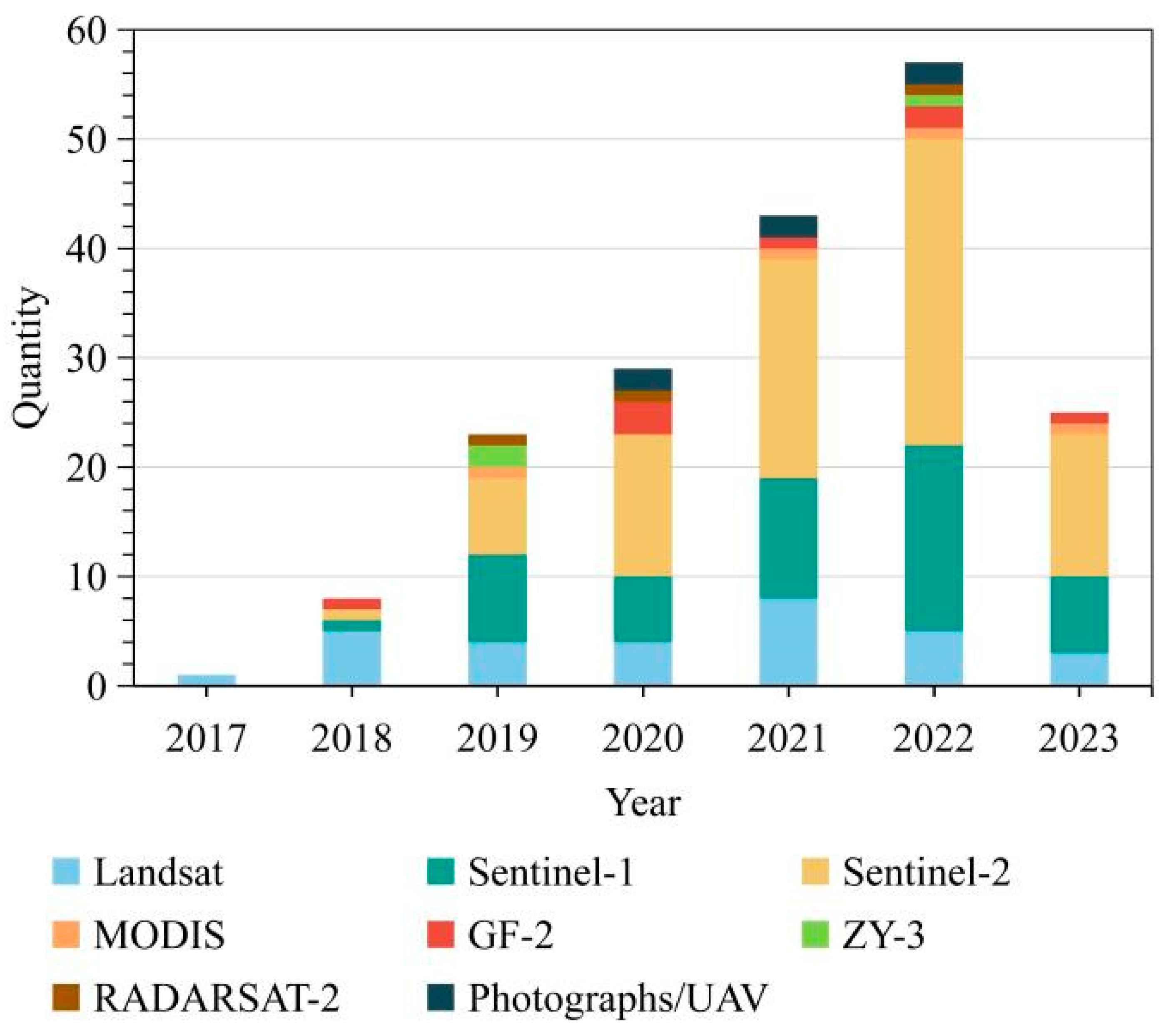
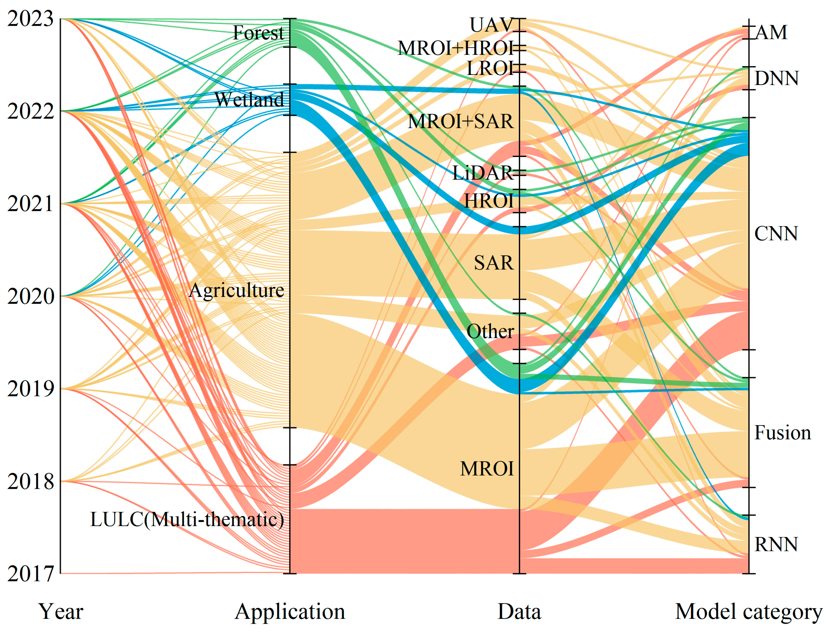
2. Statistics from the Literature

This review is based on the literature obtained by searching the Web of Science (up to 20 June 2023). The search formula was: (TS = (deep learning) OR TS = (neural network)) AND (TS = (multitemporal) OR TS = (time series)) AND TS = (remote sensing) AND TS = (classification). We filtered out papers that did not meet prespecified criteria based on their titles, abstracts, and keywords. In total, this review includes a total of 170 studies. As a relatively new research field, the use of deep learning for remote sensing multitemporal classification has developed rapidly in recent years (Figure 1a). It should be noted that only some of the literature published in 2023 is included in the chart shown in Figure 1a. By constructing a relationship map of keywords (Figure 1b), we determined that 30 keywords included in the papers are divided into four groups represented by “deep learning”, “classification”, “random forest”, and “land-cover classification”. The green area representing “deep learning” shows that CNNs have been widely used and that deep learning is more targeted at time dimension analysis of multitemporal data. The blue group representing “classification” presents the data sources and application directions of multitemporal classification. Agricultural mapping and land cover are the main application directions for classification, with Sentinel-1, Sentinel-2, and their combination being commonly used data sources for multitemporal classification. The red area clusters keywords related to model application verification. Random forest is widely used as a comparative model to verify the effectiveness of deep learning models. It also provides evidence supporting the model’s advancement by verifying the accuracy of image classification results. Vegetation in China is often used as a verification and application object for these models. In addition, the two keywords “land-cover classification” and “neural network” are separately grouped because they respectively contain and summarize the relationship between classification applications and deep learning.

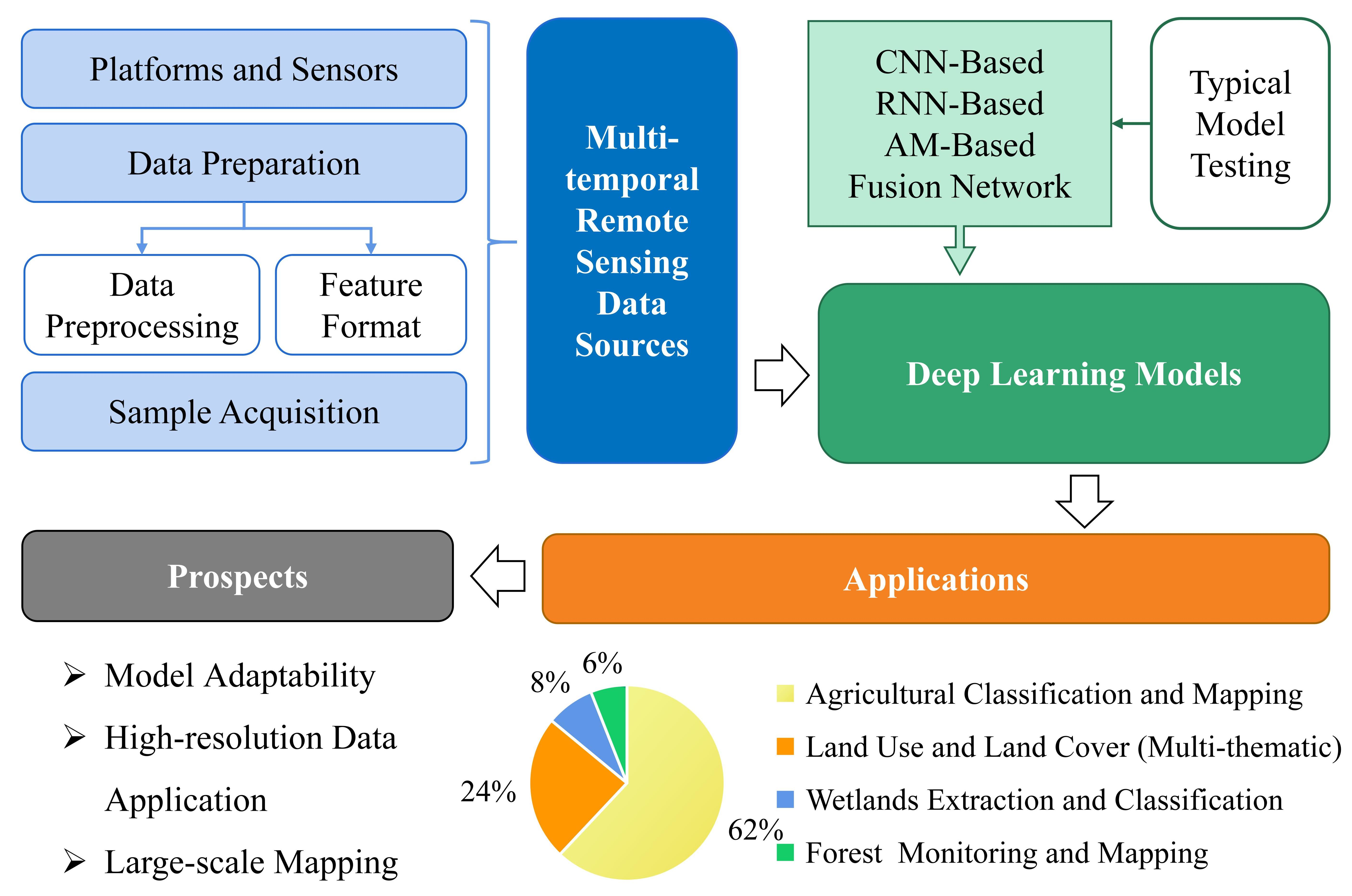
3. Remote Sensing Data Sources

3.1. Remote Sensing Platforms and Sensors

Optical imagery, synthetic aperture radar (SAR), and light detection and ranging (LiDAR) are three widely used remote sensing imaging technologies. In multitemporal image classification, satellite images used for deep learning mainly come from satellites such as Landsat5 and 8, Sentinel-1 and -2, GF-1 and -2, etc. (Figure 2). Among them, Sentinel-2 is the most popular because of its superior spatial and temporal resolution [31]. Sentinel data are widely used because they are freely available and have higher resolution than Landsat data.

Table 2. Satellites used and their information statistics obtained from the papers included in this review.

Image Type	Name	Launch Year	Temporal Resolution	Pixel Spatial Resolution
MROI	Landsat5	1984	16 days	MS resolution: 30 m LWI: 120 m
MROI	Landsat7	1999	16 days	Panchromatic resolution: 15 m MS resolution: 30 m
LROI	Terra/Aqua (MODIS)	1999/ 2002	1–2 days	Depends on the band: 250 m to 1000 m
HROI	Formosat-2	2004	Daily	Panchromatic resolution: 2 m MS resolution: 8 m
SAR	COSMO-SkyMed	2007–2010	16 days	Depends on the operational mode The best resolution for stripmap mode (Himage): 3 m
SAR	RadarSat-2	2007	24 days	Full polarization mode resolution: 8 m
MROI+HSI	HJ-1 A/B	2008	Single satellite: 4 days HJ-1 A and B: 2 days	RGB-NIR resolution (CCD): 30 m HSI resolution: 100 m IRS resolution: 150–300 m
HROI	Worldview-2	2009	1.1 days	Panchromatic resolution: 0.46 m MS resolution: 1.84 m
HROI	ZY3	2012	5 days	Panchromatic resolution: 2.1 m MS resolution: 5.8 m
MROI	Landsat8	2013	16 days	Panchromatic resolution: 15 m MS resolution: 30 m
HROI	GF-1	2013	4 days	Panchromatic resolution: 2 m MS resolution: 8 m
HROI	GF-2	2014	5 days	Panchromatic resolution: 0.8 m MS resolution: 3.2 m
HROI	Worldview-3	2014	Daily	Panchromatic resolution: 0.31 m MS resolution: 1.24 m
SAR	Sentinel-1	2014	Single satellite: 12 days S1A and B: 6 days	Depends on the operational mode The best resolution for stripmap mode: 5 m
MROI	Sentinel-2	2015	Single satellite: 10 days S2A and B: 5 days	Depends on the band: 10 m to 60 m RGB-NIR resolution: 10 m
MROI	VENμS	2017	2 days	10 m

HROI: high-resolution optical imagery; MROI: medium-resolution optical imagery; LROI: low-resolution optical imagery; HSI: hyperspectral imagery; MS: multi spectral; LWIR: longwave infrared; IRS: infrared radiation sensor.

provides an overview of these satellites and their image products. Most of the satellite products in the table are multispectral images. Among them, Sentinel-1, RadarSat-2, COSMO-SkyMed, and HJ-1 A/B can generate SAR and hyperspectral images. Landsat, WorldView, ZY3, GF, and Formosat-2 can generate panchromatic images, which usually have higher spatial resolution than multispectral images. Due to the limitations of sensor observation capabilities, orbital characteristics of observation platforms, and clouds and their shadows, most remote sensors only have minimum point observation capabilities. Studies have shown that linking surface reflectance anisotropy with land cover or NDVI can help extract prior knowledge from historical bidirectional reflectance distribution function (BRDF) products, thus improving the retrieval of surface reflectance [32]. MODIS maximizes the use of BRDF characteristics of the surface by providing multi-angle information from the sensor.

In addition to satellite remote sensing, unmanned aerial vehicle (UAV) remote sensing and LiDAR have also been applied in this field. UAV remote sensing has the advantages of low cost, high spatial resolution, and the ability to repeat acquisitions. It has been used for crop growth evaluation in the agricultural field [33,34]. LiDAR includes terrestrial laser scanning (TLS) and airborne and spaceborne laser radar. Since the launch of satellites such as GEDI and ICEsat2, the availability of remote laser radar data has been increasing, providing another source of information [35]. LiDAR not only provides more land cover information but also captures detailed 3D information about the landscape. It has a wide range of applications in land cover classification, forestry, and ecology [36,37]. Deep learning models and multitemporal data from UAV and LiDAR are commonly combined in crop classification [38,39,40], land cover classification [41], tree feature separation [42], and other fields.

In addition to the traditional remote sensing methods, sonar devices, such as SAS (synthetic aperture sonar) [43,44] and SSS (side scan sonar) [45], are usually used for underwater object recognition and classification. Usually, time domain, wavelet, time-frequency analysis, and other processing methods use a target signal to extract features or feature visualization for underwater target recognition, environmental detection, and so on [46]. To utilize the time dimension information of sonar signals, time domain, frequency domain, time-frequency domain, and auditory samples can be extracted from each frame and stacked according to the time sequence to improve the robustness of a deep learning model [47]. The main purpose of applying acoustic image sequences is to improve the appearance of underwater targets and minimize clutter noise [48,49].

3.2. Preparation of Multitemporal Remote Sensing Datasets

3.2.1. Atmospheric Correction

Due to scattering and absorption, electromagnetic radiation is easily affected by the composition of gases and aerosols in the atmosphere during ground observation [50]. This not only makes it difficult to compare measurement results from different optical sensors but also has a negative impact on research results in large-scale remote sensing data applications (such as multitemporal remote sensing data applications) [51]. In order to reduce the influence of the atmosphere, atmospheric correction is used as a common preprocessing step before multitemporal classification.

Satellite image atmospheric correction methods are mainly divided into empirical methods and model-based methods. Among them, the radiative transfer (RT) model does not rely on on-site spectral measurements. Based on the RT model, many atmospheric correction tools have been developed that can provide reliable atmospheric correction results [52]. For example, when using Sentinel-2 images, the data are usually corrected for atmospheric effects using the Sen2Cor module of SNAP (Sentinel Application Platform) based on level1c data, or the surface reflectance is preprocessed using MAMJ (MACCS ATCOR Joint Algorithm) developed by CNES (Centre National d’Études Spatiales). Landsat5 and 7 usually use software such as ENVI and FLAASH to calculate atmospheric transmission parameters using the 6s (Second Simulation of a Satellite Signal in the Solar Spectrum) model or the MODTRAN (MODerate resolution atmospheric TRANsmission) model. However, an atmospheric correction tool should be selected according to the actual application scenario depending on its performance on different land targets. Sola et al. [51] evaluated the atmospheric correction method for Sentinel-2 level1c using six different land cover types and found that MAMJ performed best among algorithms such as Sen2Cor and 6s. Moravec et al. [53] tested six atmospheric correction methods on Landsat8 and Sentinel-2 data for their impact on NDVI. In addition to the satellites mentioned above, data from GF, ZY-3, and other satellites are usually preprocessed using software provided by manufacturers. The atmospheric correction methods vary depending on the characteristics of satellite sensors and data processing requirements.

Claverie et al. [54] proposed the Harmonized Landsat and Sentinel-2 (HLS) project, which combines Landsat and Sentinel-2 product observations into one dataset, greatly reducing time errors caused by atmospheric correction methods. The product has great potential in research requiring high temporal and spatial resolution. After atmospheric correction, MODIS data produce many derived products, such as MOD09/MYD09 and MOD17/MYD17.

For multitemporal images, it is important to adjust the atmospheric correction parameters for different seasons to suit different atmospheric conditions. Comparisons between the results of atmospheric correction and ground observation data or other independent correction references are important to improve the accuracy of correction.

3.2.2. Removing Clouds and Noise

Research using multitemporal imagery requires a continuous stream of images over time. For optical remote sensing images, it is difficult to avoid cloud, snow, and shadow coverage. Although historical satellite images are readily available, missing or discontinuous data may still occur due to noisy observations, leading to poor target identification and classification, so data preprocessing is vital [55]. Specific preprocessing methods include:

• Directly removing cloud-covered images or setting a threshold to remove cloudy images when a sufficient number of available images are present [56,57,58,59]. This method has a high calculation rate and is easy to implement. However, its shortcomings are that setting the threshold requires a lot of prior knowledge and human participation, and it is highly subjective.
• Filling in the cloudy portions of observations using linear time interpolation after cloud removal [5,60,61]. The implementation of this method first requires that the selected multiple images have a certain degree of temporal continuity. In addition, if there is an overlap of cloud areas in multiple periods of images, then this method cannot eliminate the impact of clouds.
• Synthesizing cloud-free images from multiple images [62,63,64]. The synthesis of multiple images needs to solve the registration and correction problems between different images and also the radiation differences between the original images and the corrected images.
• Replacing noisy images with higher quality images from a neighboring year on the same date [65,66]. Due to the fact that clouds often gather during the rainy season, it is difficult to ensure the quality of images near the same date in adjacent years. Moreover, when there is a significant change in the land cover type near the same date in adjacent years, it will seriously affect the classification results.
• Sending the cloud noise portion of the data to deep learning models for learning [66] or using it as noise limitation in the model [16,67,68]. Compared with traditional methods, deep learning methods have stronger robustness and can achieve higher accuracy. However, for deep learning-based methods, building models with strong generalization ability on time and space scales is still a challenge in cloud and cloud shadow detection methods.

3.2.3. Multisource Data Fusion

Data fusion can combine complementary information contained in different types of data to help improve the discriminability between different land cover categories. Optical images are still the most common multitemporal remote sensing data used for land cover classification. In recent years, SAR data have gradually been applied in multitemporal image analysis due to their excellent texture expression ability and all-weather characteristics [69]. The fusion of optical images and SAR data makes full use of the characteristics of land cover, improves the separability of land cover, and makes up for the image loss caused by weather conditions in multiple time series. LiDAR can characterize the three-dimensional structure of targets and has been proven to be advantageous for identifying categories with small morphological changes [41]. With the maturity of airborne LiDAR technology, the combination of airborne LiDAR and optical images has proved to be effective in the field of land use classification. Jin et al. [70] combined optical images, including optical images, SAR, and LiDAR, and the discrimination ability when using integrated data for different land cover types was significantly better than the dual-sensor and single-sensor classification accuracy, especially for enhanced vegetation category recognition.

The second way to use multi-source data is by combining two similar sensors, which is achieved with the following two fusion methods:

• Analyze the performance of different resolution data sources in deep learning models separately to test the robustness of the model.
• Fuse high-temporal-resolution and high-spatial-resolution images to obtain high-quality images and improve classification accuracy [55,71,72]. In addition, some other products (such as terrain and meteorological products) and small-scale, high-precision images from UAVs are gradually combined for use in this field [73,74,75].

Although richer data sources can obtain more information about land cover, this inevitably leads to longer training processes and more stringent data conditions. How to extract useful information from multi-source data to remove redundant information and improve training efficiency is a problem that needs to be solved at present.

3.2.4. Dimensionality Reduction and Feature Extraction

Multitemporal images have rich temporal features, which also significantly increases the amount of data. When training deep learning models, multitemporal images are usually stacked along the time dimension and trained on a per-pixel or multidimensional image block basis [12,76,77]. This method ensures data integrity and reduces the difficulty of manually selecting features, but it often leads to data redundancy and increased computation costs. Moreover, with an increase in feature dimensions, the classification accuracy will show the phenomenon of “first increase and then decrease” (Hughes phenomenon) [78].

Some studies choose to extract new features from the original remote-sensing images to form time series curves with different features. The purpose is to use expert knowledge to improve the efficiency of feature extraction. When the original remote sensing image is an optical image, specific indices such as the normalized difference vegetation index (NDVI), enhanced vegetation index (EVI), normalized difference water index (NDWI), and normalized emissivity (NaE) are usually obtained using band operations [63,64,75,79,80]. SAR data usually use polarization features such as VV, VH, and VH/VV [74,75,81] or directly extract features such as the mean and standard deviation [74,82,83]. However, it should be noted that additional feature extraction may result in information loss, leading to a decrease in model accuracy.

Projection-based methods can use mathematical transformations to obtain a new set of low-dimensional feature combinations. Common methods include PCA (principal component analysis), SCA (spectral correlation angle), WT (wavelet transform), etc. Song et al. [84] used PCA and SCA to screen spatiotemporal spectral features. Bazzi et al. [85] combined PCA and WT with random forests and applied them to multitemporal irrigation area mapping. These methods are relatively simple to operate and widely used, but they cannot effectively describe the features of subtle land cover types. In contrast, feature extraction methods based on popular learning and deep learning have better extraction effects, but the disadvantages are that parameter settings are required and that the complexity is high. It should be noted that additional feature extraction work will not only make the operation process more complicated but may also cause information loss, resulting in a decrease in model accuracy [24,86].

3.2.5. Input Format for Deep Learning Models

Tian et al. [87] classified the model feature input form into scene-based methods and pixel-based methods. That is, before training a model, the multi-dimensional feature data set of T × C × H × W (time × channel number × height × width) is synthesized from the image (where the channel number refers to the number of bands or features) or the pixel feature time series that meets special conditions is extracted. Based on this classification, this review divides the deep learning model input for multitemporal remote sensing classification into three types: pixel-level, image block-level, and a combination of both.

The first type, per-pixel multitemporal image classification, is commonly seen in RNN-based models and Conv1D, which train a sample set by iterating over the multichannel and time-series information of each pixel. For a single training batch, the time series information of multiple bands of a single pixel is combined and input into the model for training, with the data format being T × C (time × channel) [5,88,89,90].

The second type of image block-level model is commonly used in 3D CNNs. This type of model typically requires image segmentation before training. The time-series image is cropped with overlap or nonoverlap using a sliding window. This step is necessary because a large amount of data from multidimensional datasets can cause insufficient computer memory during a single batch input. After segmentation, the segmented image set is added to the model for training in batches. The data format for a single input is T × C × L × L (time × channel × the size of image blocks) [41,91,92].

The third type is a combination of the first two and is typically a composite model of a CNN and RNN (or Conv1D). Inputs for this type of model are roughly divided into two types: the first type combines a CNN and RNN into a seamlessly connected model, where the time series and multichannel information of each pixel are extracted and input into the RNN (or Conv1D) model to obtain an image with multiple time dimensions. This multi-feature image is then input into the CNN model, and spatial features are obtained using spatial convolution [41,91,92,93,94]. The second type simultaneously inputs data in both pixel and image block formats into the corresponding models for training, and the classification scores for the target are calculated using a fully connected layer (FC layer) to complete the classification task [60,62,95].

In deep learning models, the data are generally divided into three parts before training: the training, validation, and test sets. The training set is used to train the individual classification algorithm, the validation set is used to select the best hyperparameters, and the test set is used to evaluate the final classification results. Dataset partitioning needs to follow two principles: (a) the sets are independent of each other and (b) the class distribution in all sets is similar [96].

3.3. Sample Acquisition

3.3.1. Manual Collection of Samples

In terms of sample acquisition, manual collection of samples is a common practice. Samples are often collected during on-site inspections using devices such as GPS (Global Positioning System) [64,88,95,97] or by manually outlining polygons as training data [62,75]. In addition, visual interpretation of high-resolution imagery is also used as a means for sample acquisition [95]. However, this approach requires a certain level of expertise and a thorough understanding of the optical properties of objects on the ground to ensure the accuracy of the samples, thereby ensuring the reliability of the training process. To achieve better training results, data augmentation (DA) techniques can be used to expand the sample set. For remote sensing imagery, methods such as rotation, cropping, contrast transformation, and false-color image synthesis can be used for data augmentation [98]. The synthetic minority oversampling technique (SMOTE) is commonly used to artificially generate new samples to deal with the problem caused by imbalanced samples. Building upon this, stratified SMOTE is proposed to address the issue related to SMOTE over increasing the number of rare land classes, which can be resolved using stratified sampling of land cover types [73].

3.3.2. Open Sample Datasets

However, whether obtained using field exploration or reference data, training samples are selected manually based on limited experience and knowledge, and it cannot be guaranteed that the selected samples effectively represent the corresponding land cover categories. Some studies [61,99,100,101] have used open sample datasets as training samples to address the time-consuming and labor-intensive nature of field surveys and visual interpretation as well as the need for specialized knowledge [55]. In this review, we examined 11 open-access sample datasets for agricultural and land cover categories and provide a brief introduction to the basic information in these datasets (

Table 3. Common agricultural and land use sample datasets.

Name	Type	Year	Region	Spatial Resolution /Data Quantity	Classifications	Link
China’s Multi-Period Land Use Land Cover Remote Sensing Monitoring Data Set	LULC	1980–2015 (five years)	China	0.05°	6 primary classes and 25 secondary classes	https://data.tpdc.ac.cn/zh-hans/data/a75843b4-6591-4a69-a5e4-6f94099ddc2d/ (accessed on 11 February 2023)
Cropland Data Layer	Crop	1997–2021 (yearly)	USA	The CDL has a ground resolution of 30 or 56 m depending on the state and year.	131 crop types	https://nassgeodata.gmu.edu/CropScape (accessed on 8 February 2023)
ChinaCropPhen	Crop	2000–2015	China	1 km	Wheat, corn, and rice	https://doi.org/10.6084/m9.figshare.8313530 (accessed on 8 February 2023)
Land Use and Land Cover Survey	LULC	2001–2018 (three years)	European Union	The 2009–2015 field surveys consisted of around 67,000 points.The ongoing Lucas survey 2018 is based on 337,854 points/observations.	7/10/16 land cover classes	https://ec.europa.eu/eurostat/web/lucas (accessed on 10 February 2023)
Land Parcel Identification System	Crop	2005–2020 (yearly)	European Union	The level of detail for crop types varies from country to country.
Annual Crop Inventory	Crop	2009–2021	Canada	30 m (56 m in 2009 and 2010)	72 classes of land (52 crop types)	https://open.canada.ca/en/apps/aafc-crop-inventory (accessed on 8 February 2023)
California Department of Water Resources	LULC/Crop	2014, 2016, 2018, 2019 (Statewide) 2015, 2017 (Delta)	California, USA	40 w+ parcels	256 land cover classes, 13 crop types, and one other category	https://gis.water.ca.gov/app/CADWRLandUseViewer (accessed on 8 February 2023)
Satellite Image Time Series with Pixel-Set and patch format	Crop	2017	Southern France	191,703 individual parcels (24 dates)	20 classes nomenclature designed by the subsidy allocation au-thority of France	https://github.com/VSainteuf/pytorch-psetae (accessed on 8 February 2023)
FROM-GLC10	LULC	2017	Global	10 m	10 land cover classes	http://data.ess.tsinghua.edu.cn (accessed on 8 February 2023)
ZueriCrop	Crop	2019	Swiss Cantons of Zurich and Thurgau	28,000 parcels	48 crop types	https://polybox.ethz.ch/index.php/s/uXfdr2AcXE3QNB6 (accessed on 10 February 2023)
MT-RS dataset from 2021 IEEE GRSS Data Fusion Contest	LULC	2019	Maryland, USA	2250 different tiles (each one covering approximately a 4 km × 4 km area)	15 classes including various forest and developed categories	https://www.grss-ieee.org/community/technical-committees/2021-ieee-grss-data-fusion-contest-track-msd/ (accessed on 10 February 2023)

).

3.3.3. Semi-, Self-, and Unsupervised Learning

Deep learning requires a large amount of labeled data to train models. Most of the current studies still use field surveys and visual interpretation to obtain labeled samples, which require a lot of manpower, material resources, and expert knowledge, making these methods unsuitable for large-scale mapping. Some studies use existing datasets to solve the problem of manual labeling. However, few land cover and crop-type datasets can meet the requirements for large-scale and detailed classification. Taking crop classification as an example, only a few countries (such as the United States and Canada) provide annually updated crop type maps. In other countries, the ability to timely collect ground annotations and generate accurate crop-type maps is not easily obtained [61,102]. Moreover, during the sample labeling process, noise may still be generated and affect the training effect of the model. At present, in order to alleviate this problem, research is gradually developing toward semi-supervised, self-supervised, and unsupervised learning.

Usually, semi-supervised learning integrates unlabeled data based on a limited number of labeled data to generate more samples to improve learning accuracy [103]. Traditional semi-supervised methods are based on a small number of field samples, which calculate similarity and set thresholds to extract unlabeled samples and expand the number of samples [88]. In addition, spectrometers can be used to obtain the standard spectral characteristics of typical objects in the field [104], and similarity calculation methods such as DTW can be used to extract unlabeled samples around the sample points or plots. Based on this, Ji et al. [91] used a cyclic training method to add the extracted samples that were confirmed manually to the sample set. In recent years, semi-supervised learning models have been developed that complete classification tasks using existing samples and unlabeled data [55].

The difference between self-supervised learning and semi-supervised learning is that self-supervised learning uses a large amount of unlabeled data to train models and then transfers the model to supervised downstream tasks. Y. Wang et al. [105] divided self-supervised learning into three categories: generative, predictive, and contrastive methods. Li et al. [106] used GAN generative models as discriminators to reconstruct images to learn multitemporal image information. Yuan & Lin [57] used temporal context information to design pretext tasks to complete image classification with fine-tuning on a small number of samples. Although generative models excessively generate information unrelated to classification, predictive models use pretext tasks to make the model learn features specifically. However, the performance of predictive models depends on the design of pretext tasks and lacks generalization ability. The contrastive method completes classification by learning the similarity of input semantics [55]. This method performed well in unsupervised semantic segmentation but has not yet been applied in multitemporal image classification.

In addition, transfer learning uses cross-domain datasets for transfer learning and completes classification by transferring learning from domain datasets similar to classification tasks. For example, Jiang et al. Jiang et al. [107] used parameter-based transfer learning and a modified National Institute of Standards and Technology (MNIST) database to establish a pre-trained model for classifying EVI time series curves. The classification effect of transfer learning depends on the gap between domains. Even if pre-training on cross-domain datasets can improve classification performance, better classification results will be obtained if remote sensing datasets are used [108]. Therefore, large-scale remote sensing datasets are also an important tool for researching the performance of remote sensing classification models.

Unsupervised classification algorithms are used to cluster elements based on similar attributes without any prior knowledge. This method is commonly used for target feature extraction in remote sensing scene classification, but when the unknown image is not classified with sample data, its accuracy is poorer than supervised classification results.

The above methods have alleviated the dependence of deep learning models on sample data to a certain extent. In the past training process, the quality of sample data greatly affected the training results. Whether it is transfer learning or unsupervised classification, the proportion of applications in multitemporal image classification is small and still mainly takes the form of supervised learning. Autonomous sample selection methods, cross-domain sample utilization, unsupervised clustering models, etc., have reduced the pressure on manual sample acquisition and have great development potential in large-scale classification applications in the future.

4. Overview and Testing of Deep Learning Models for Multitemporal Remote Sensing Classification

Data-driven deep neural networks are helpful in identifying fundamental sequential dependencies from multitemporal remote sensing observations. In time-series deep learning for remote sensing classification applications, the input layer initially takes the remote sensing data, and the output layer produces the predicted classification. The hidden layers in between transform the feature space of the input to match the output. Deep learning shifts the focus from what the model should learn to how the model should learn. RNNs, CNNs, self-attention networks, and their variants are popular deep-learning architectures for handling time-series satellite data [101]. This section provides an overview of the models that are frequently used in this field, including CNN-based models, RNN-based models, attention mechanisms, and multi-model combinations. According to the number of times each model type was used per year (Figure 3), the proportion of CNN-based models has increased year by year, indicating that CNN models are more suitable for multitemporal classification. RNN-based models received a lot of attention in the beginning, but their usage has decreased in recent years. AM was developed later and its application (usually the Transformer model) represents a certain proportion of the research reviewed in this article. A fusion model is designed by combining multiple models into a single model architecture, which is generally a CNN+RNN model architecture.

4.1. CNN-Based Network Models

Since AlexNet won the ImageNet competition in 2012, deep neural networks have achieved many successful applications in various fields [68,109]. Following the success of these CNN architectures in different domains, researchers started to use them for time series analysis. In past studies, convolutional layers in CNN models mainly acted as feature extractors in the spatial or spectral domain but were rarely applied in the temporal domain of remote sensing time series [5]. In recent years, CNN models such as FCN and ResNet, as well as their variant models, have been increasingly used in multitemporal remote sensing classification.

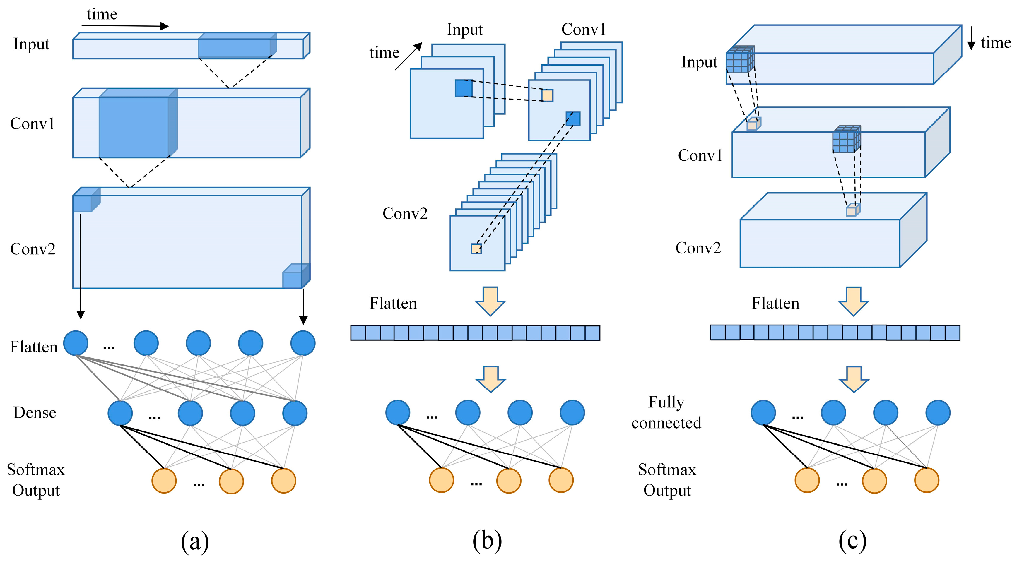
4.1.1. One-Dimensional and Multidimensional Convolution

In multitemporal remote sensing classification, convolution on the temporal axis can be viewed as sliding filtering on the time series or as multidimensional convolution blocks performing spatio-spectral multidimensional sliding filtering. Unlike images, filters only exhibit one dimension (i.e., time, as shown in Figure 4a) instead of two dimensions (i.e., width and height, as shown in Figure 4b). Filters can also be regarded as a general nonlinear transformation of time series [110]. Conv1D [66,111] and temporal convolutional neural networks (TempCNNs) [17] are commonly used to apply convolutional kernels to capture temporal patterns or shapes in input sequences. Deep features are gradually extracted from multiple convolutional layers, patterns are matched with inputs using convolution, and then classification is finally completed. Meanwhile, multidimensional convolution kernels can obtain contextual information about surrounding pixels from more dimensions (Figure 4c). This ability to utilize information within the convolutional kernel often yields better classification results [68]. Ji et al. [94] extended the application to multivariate time series and proposed a 3D CNN, which was shown to outperform a 2D CNN and other classical methods. Adrian et al. [68] achieved excellent classification accuracy for multitemporal crop classification using 3D U-Net (with 2D U-Net and 2D SegNet as comparison models).

4.1.2. Other CNN Models

CNNs were developed earlier in multi-class deep neural networks and have been widely used. Many improved models have been developed. They are mainly divided into traditional CNN models (AlexNet, VGG), fully convolutional network models (FCN), encoder–decoder models (U-Net, SegNet), and short-cut networks (ResNet, DenseNet, DPN). This review summarizes and classifies the typical models that are widely applied, as listed in

Table 4. Typical CNN-based improved models applied to multitemporal remote sensing classification.

Types	Name	Advantages	Weaknesses	References
Early CNNs	AlexNet [109]	It can avoid overfitting and improve training speed by discarding units randomly	The network depth is shallow, leading to low classification accuracy	[60,62,66,95,112,113]
	VGG [114]	Nonlinear fitting ability is improved by stacking convolution kernels continuously	The training speed is slow
Fully Convolutional Networks (FCNs)	FCN [115]	The number of parameters is invariant and can be used for transfer learning; contains more parameters than DCNN	It is not sensitive enough to image details and does not consider the spatial relationships between pixels	[116,117,118,119]
Encoder–Decoder	U-Net [120]	The U-shaped network structure is useful for extracting the spatial and temporal features effectively and outperforms 2D-CNN; a 3D U-Net can identify different temporal features in heterogeneous crop types	Training speed is slow and less contextual information is obtained	[99,121,122,123]
	SegNet [124]	Encoder–decoder architecture has advantages in multitemporal classification as it allows a more progressive reconstruction of spatial information	The model is large and requires more computer memory	[68,83]
Short-cut	ResNet [125]	Uses hopping connections to avoid gradient explosions caused by increasing the number of neural network layers	It requires a lot of computing resources to train, the effective sensing field is not deep enough, nd it depends heavily on the parameter settings	[42,126,127]
	DenseNet [128]	Each layer is densely connected to the rest to ensure maximum flow of information between layers; the features can be transferred more effectively, which is beneficial for improving the information flow and gradient	The structure is more complex and requires more computing resources and time	[129,130,131]
	Dual Path Networks (DPNs) [132]	It combines the characteristics of ResNet and DenseNet, which can propagate gradients to the deeper level	Requires a lot of computing resources	[17]
Dilated convolution	DeepLab [133]	Void convolution is used to avoid information loss without increasing the number of parameters	Requires a lot of computing resources	[134]
Pyramid network	Feature Pyramid Network (FPN) [135]	It is a hierarchical structure with top-down horizontal connections that add precise spatial information to the segmentation	There is a semantic gap between different layers, and the downsampling process will lose the feature information of top-level pyramid	[136,137,138]
	Pyramid Attention Network (PAN) [139]	Propagation of low-level features is improved by enhanced bottom-up paths	The path of information from the bottom to the top is long

, and lists the literature on their applications in multitemporal remote sensing classification.

4.2. RNN-Based Network Models

In traditional multi-layer neural networks, all inputs belonging to a time series are considered independent of each other, so these networks cannot take advantage of the inherent dependencies between inputs when processing sequential data. RNN-based network models are another class of neural networks that extend traditional networks using loops in their connections (Figure 5a,c) [140,141]. RNNs are specifically designed for sequence data analysis and have recently been successfully used in some remote sensing classifications. RNNs can represent data in continuous dimensions and have sequential dependencies. The most common approach of an RNN is to extract features from multiple time observations in the time domain as the model can effectively handle sequential data. However, due to gradient vanishment and explosion during the backpropagation process in the training phase of an RNN, traditional RNNs cannot handle long-term dependencies [67]. A special type of RNN called long short-term memory (LSTM) [142] can overcome these problems and has been widely applied in recent research.

LSTM preserves the temporal features in long time series by introducing gated modules. The model stores information in LSTM cells at the current time step and adaptively passes it to the next cell based on gating weights to gradually accumulate temporal correlations of complete input sequences (Figure 5a,d). Using self-learned gating parameters, the LSTM model can stably retain key temporal features throughout its recurrent flow for both long-term and short-term memory. The multitemporal structure of LSTM models naturally matches multitemporal satellite observations with crop growth processes [5]. As a result, LSTM models have been extensively explored in recent multitemporal crop mapping studies [17,75,79,100,143,144,145,146]. LSTM models extract sequential relationships between multiple time observations to automatically identify cloud pixels for robust crop mapping performance [16]. Single crop identification, such as corn and sugarcane, can be achieved by learning the cumulative characteristics of time-series remote sensing data using multi-time LSTM models [72,147].

Based on LSTM, a large number of optimized models have been developed. They include gated recurrent unit (GRU) [148], bidirectional LSTM (BiLSTM) [149] and Im-BiLSTM [97]. These models optimize the LSTM model from different directions.

Table 5. Applications of LSTM model variants in multitemporal remote sensing classification.

Name	Advantages	Weaknesses	References
GRU	It has fewer parameters, so training is slightly faster and it requires less data to generalize	Classification accuracy may be lower than LSTM	[60,143,145,146]
BiLSTM	It can extract temporal characteristics before and after and achieves good results in rice recognition	It requires a lot of computational memory	[150,151,152]
Im-BiLSTM	The combination of BiLSTM and a fully connected interpolation layer has achieved good performance in multitemporal crop mapping	Imputing missing data requires additional computing resources, and the quality of the imputed data will affect the final classification accuracy	[97]

summarizes the performance of these three types of models and lists the literature on their applications in multitemporal remote sensing classification.

4.3. Attention Mechanism

4.3.1. Attention Mechanism

The attention mechanism mimics the human visual system by focusing weights on important information. In other words, it assigns higher weights to relevant parts while minimizing irrelevant ones by assigning them lower weights [153]. The application of attention mechanisms in multitemporal remote sensing can be divided into two main types: channel attention and spatial attention. Channel attention networks aim to enhance feature layers (channels) that convey more important information in feature maps and silence other feature layers (channels). Spatial attention networks highlight regions of interest in feature space and mask background areas. These two attention mechanisms can be used separately or combined in DL methods to provide attention to important feature layers and locations of regions of interest. Attention mechanisms are often used in combination with other models:

• In a study on multitemporal message classification using CNNs combined with attention mechanisms, W. Zhang et al. [71] used channel attention modules to emphasize meaningful bands for better representation and classification of SITS. Channel attention modules and spectral–temporal feature learning were used. The former was used to learn band weights and focus the model on valuable band information. In the latter, dynamic aggregation blocks effectively extracted and fused features from the time dimension. Meanwhile, Seydi et al. [59] proposed a new AM framework for extracting deep information features; both spatial and channel attentions were embedded into a CNN with different attention network designs. For a CNN, channel attention is usually implemented after each convolution, but spatial attention is mainly added at the end of the network [154,155,156].
• Because it uses multiple LSTM layers and an attention mechanism, the AtLSTM model improves the distribution of temporal features learned from the LSTM layer by introducing an attention module that adjusts the contribution of hidden features by normalizing weights. The attention module consists of a fully connected layer with softmax activation that generates attention weights for each hidden feature produced by LSTM layers. The learned features outputted by the attention module are fed into a fully connected layer and softmax function to produce normalized prediction scores for potential target classes. The class with the highest score is selected as the predicted class. It aims to discover complex temporal representations and learn long-term correlations from multi-time satellite data and has been widely applied [61,64,101,130]. In addition, the time attention encoder (TAE) incorporates a self-attention mechanism. This concept emphasizes relationships between different positions in input sequences (here, time series) for computing sequence representations.

4.3.2. Transformer

The Transformer model consists of an input module, an encoder module, and an output module. The encoder module achieves feature extraction by stacking multiple multi-head self-attention layers, each followed by a fully connected layer. Shortcut connections and layer normalization operations are applied after each layer. The transformed features output by the last fully connected layer are globally averaged over the time dimension and then fed into the output module to predict land cover types (Figure 6) [17,57,58,101]. The Transformer has excellent parallel training capabilities and is not affected by gradient vanishing because its gradient propagation points to all timestamps [60]. The Transformer has performed well in the field of natural language processing, but such sequence processing typically has sequence lengths of thousands. Studies have shown that the Transformer is suitable for longer time series as it does not achieve better classification results when the time series length is less than 30 [61]. With the continuous enrichment of remote sensing data in the temporal dimension, the Transformer has enormous application potential. Figure 5 shows the network structure of the Transformer in multitemporal classification (including a schematic diagram showing the multi-head attention mechanism).

4.4. Multiple Model Combinations

Combining multiple models can produce a more complete information expression. Each model has a different perception ability and can extract different types of features from the data. The combination of different DL models achieves a more generalized perception of data, thus improving classification results.

Currently, most studies that use combined models prefer the combination of CNN+RNN to enhance the utilization of image features. The initial RNN design can capture time dependence but ignores spatial context. As a supplement to an RNN, a CNN considers spatial context but ignores sequential dependence. A hybrid method combining an RNN and a CNN has been proposed to simulate spatiotemporal background in multitemporal remote sensing problems [94]. In recent years, methods combining recursive and convolutional operations have been proposed to process spatiotemporal data, namely, ConvRNN models (e.g., ConvGRU or ConvLSTM). These architectures extend recursive neural networks by including convolutional operations in recursive units and processing multidimensional data sequences instead of vector sequences [60]. These solutions have begun to attract attention in the remote sensing field. For example, in [16], a ConvRNN is used to process land cover classification from Sentinel-2 SITS and model the task as semantic segmentation. Turkoglu et al. [31] use hierarchical label structure encoding and a ConvRNN to predict three labels at different levels for each pixel, thus improving the classification performance at fine-grained levels. In addition to these combinations, modeling time before space or space before time has achieved better classification results than single network models, for example, LSTM combined with U-Net, ResNet and other CNN networks [55,56,82,94,131]. In crop classification, the change in vegetation plots over time is revealed by spectra rather than space. Thus, to perform fine-grained crop classification based on time series images, it may be more effective to first extract time features for each pixel and then extract the spatial features [93].

In addition, ensemble models can improve the robustness and reliability of classifiers by reducing the accuracy bias of individual classifiers, thereby preventing model overfitting and obtaining better generalization ability [59,62,157,158].

Table 6. Model composition and application fields of other network model combinations.

Name	Basic Model	Application	Reference
C-AENN	CNN+SAE	Crop classification	[159]
SO-UNet	U-Net+SOM	Semi-supervised forest identification	[160]
GAN Embedded CNN and LSTM	LSTM+CNN+GAN	Semi-supervised crop classification	[106]
STEGON	CNN+GAT	Land cover classification	[161]
Updated dual-branch network	AE+Transformer	Crop classification	[162]

summarizes the basic model structures and application directions for other model combinations.

4.5. Typical Model Testing

4.5.1. Data Source

Some of the typical deep learning models mentioned above were tested using Senintel-2 images from April to October 2022. The test area was located in the central part of Wichita, Kansas, USA. Two plots of about 16 km × 16 km and 9 km × 9 km were selected as the training area and test area, respectively. The 1–8 bands of Sentinel-2 were selected, and the clouds and cloud shadows in the images were identified and masked out using the QA band. The missing values were interpolated using linear interpolation and Savitzky–Golay filtering, and monthly scale sequence images were synthesized, totaling seven images. The sample data were selected from the Cropland Data Layer dataset. The main land cover types in the test area were corn, sorghum, winter wheat, fallow, and grassland. Except for these land cover types, the rest were classified as “other”. The number of pixels occupied by different land cover types is shown in

Table 7. Number of sample pixels for different land cover types.

Class	Label	Train Pixels	Test Pixels
0	Corn	711,034	209,060
1	Sorghum	102,176	35,526
2	Winter wheat	670,832	299,209
3	Fallow	539,469	343,275
4	Grassland	561,835	38,456
5	Other	89,514	25,099

.

4.5.2. Experimental Settings

The experiments were divided into land cover classifications based on image blocks and pixel-wise land cover classification. Conv2D, U-Net, DPN, Deeplabv3, ConvLSTM, and U-Net+LSTM were selected as representative models that use image blocks as input. The images were cropped into a 128 × 128 shape, the batch size was set to 30, and a total of 800 training image blocks were set. Each image block contained a total of 56 feature bands set as 7 (time) × 8 (number of bands). The representative models for pixel-wise classification were Conv1D, LSTM, GRU, and the Transformer. The batch size was set to 1000, and the size of the time series corresponding to each pixel was 7 (temporal length) × 8 (number of features). All models were trained with the Adam optimizer, using the CrossEntropyLoss loss function, and the learning rate was 0.0005. K-Fold cross-validation was used on the training set, and 10% of the training data was selected as the validation set to prevent model overfitting. The model training and testing environment configuration was Python3.8, Pytorch11.2, the graphics card was 3080ti, and the video memory was 24 g.

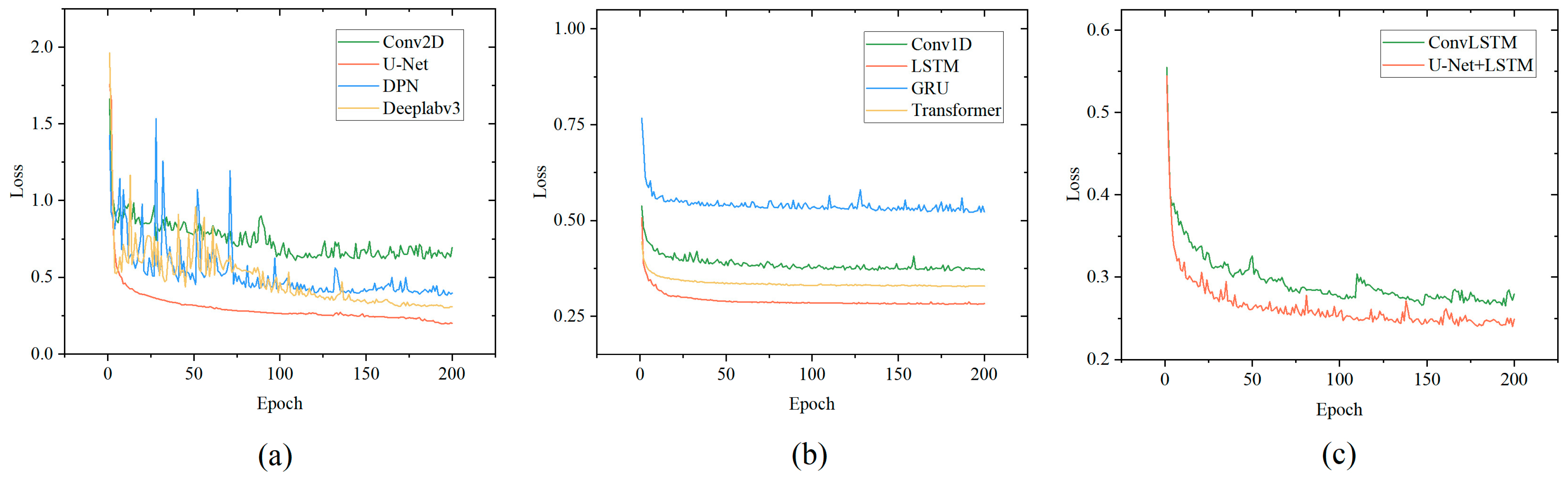
4.5.3. Test Result

As can be seen from

Table 8. Classification accuracy and running time for image block input models.

Model Category	Model Name	Input Format	OA (%)	Kappa	Train Time	Test Time
CNN-based models	Conv2D	Image block	79.81	0.7215	100 m 33 s	12 s
	U-Net	Image block	86.11	0.8063	108 m 13 s	14 s
	DPN	Image block	85.86	0.805	128 m 38 s	12 s
	Deeplabv3	Image block	85.93	0.8034	132 m	13 s
Fusion models	ConvLSTM	Image block	90.76	0.8562	131 m 44 s	15 s
	U-Net+LSTM	Image block	91.21	0.8615	239 m 46 s	14 s

, the accuracy of the fusion model was generally better than that of the single model-based accuracy, but due to the increased complexity of the model, the training time also increased. For the CNN-based models, the temporal relationship of the time series was not considered, and different times were used as feature inputs to learn spatial characteristics in the form of convolution. Among them, U-Net achieved the best classification results, with OA reaching 86.11%. The combination of U-Net and LSTM further improved the accuracy, with OA reaching 91.21%. The training efficiency of the pixel-wise models, listed in

Table 9. Classification accuracy and running time for per-pixel input models.

Model Category	Model Name	Input Format	OA (%)	Kappa	Train Time	Test Time
CNN-based models	Conv1D	Per pixel	86.89	0.8165	226 m 42 s	15 s
RNN-based models	LSTM	Per pixel	86.90	0.8158	140 m 26 s	11 s
	GRU	Per pixel	84.90	0.7884	136 m 33 s	9 s
AM-based models	Transformer	Per pixel	85.86	0.8024	1205 m 29 s	27 s

, was generally lower than that of the image block models. LSTM achieved the best classification results in a relatively short training time. These results suggest that using only multitemporal features of vegetation can achieve good classification results. Figure 7 shows the loss value decline curves for various models in the validation set. As can be seen from the figure, the CNN-based models converged slower than the RNN-type models and the Transformer. Among them, DPN and Deeplabv3 showed larger fluctuations in the early stage of the loss curve. The combined model had better classification accuracy, and corresponding to this, the loss value was also lower, but it also had relatively slower convergence speed.

5. Application

The combination of multitemporal image classification and deep learning is mainly used in agriculture, LULC (multi-thematic), wetlands and forests. The studies in each field account for 62%, 24%, 8%, and 6% of the total literature considered in this review, respectively (LULC in the following text refers to land cover and land use classification applied to multiple fields, such as identifying and classifying forests, crops, and construction land at the same time). An overview of the application of multitemporal remote sensing deep learning can be summarized according to a visualization showing the application fields and their corresponding years, data, and model categories (Figure 8). Multitemporal deep learning was first applied to LULC. This field mainly uses medium-resolution optical images (MROIs) and has maintained a stable number of applications in recent years. The various data and model categories are mainly applied to agriculture. In particular, SAR data are mainly used for agricultural classification. Wetland and forest applications started later, and the number of applications gradually increased over time. Wetland classification mainly uses MROI and SAR data and favors the use of CNN models. Forest classification involves the use of LiDAR. According to the current application status, each field is divided into more targeted research directions (Figure 9), which will be discussed in detail below.

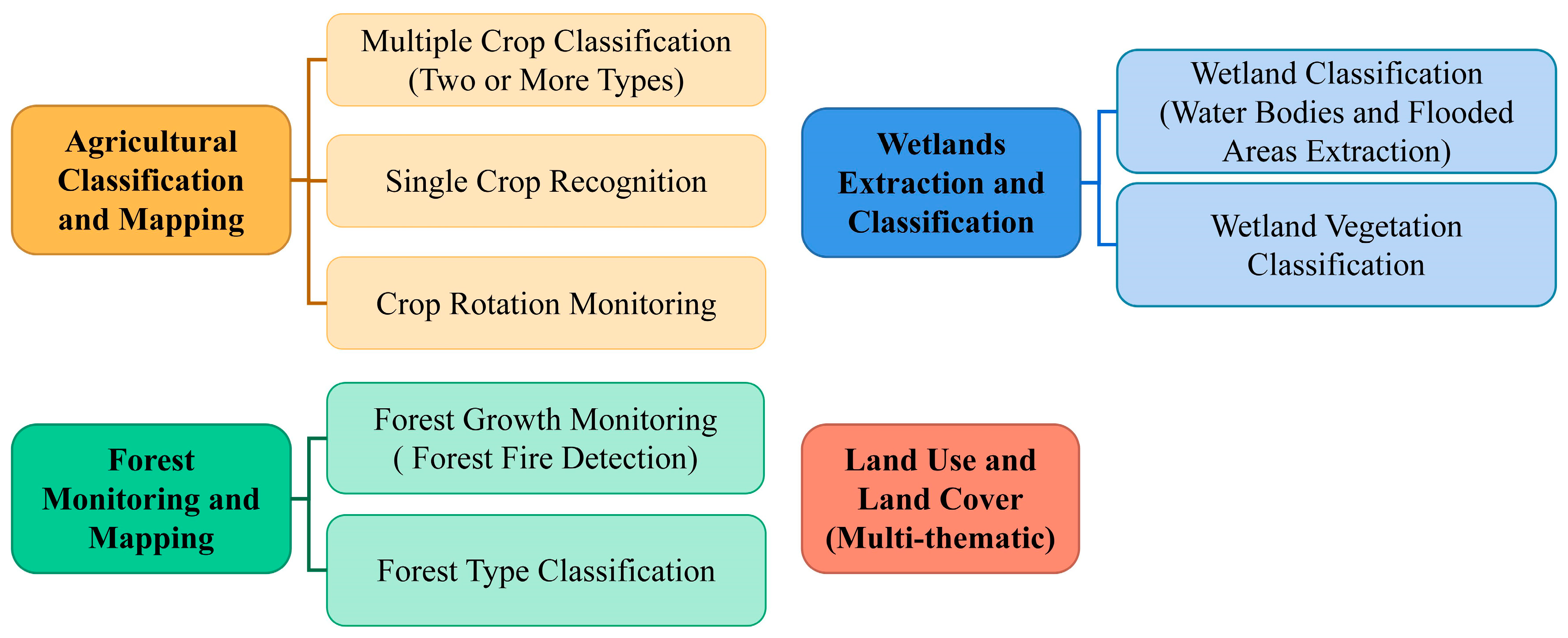
5.1. Agricultural Classification and Mapping

The spectral characteristics of vegetation are an important basis for distinguishing different types of vegetation, and seasonality is one of the most significant features of vegetation [163,164]. The spectral characteristics of each plant are highly dependent on the phenological stage of the plant [5]. Useful information about vegetation growth stages and conditions used for classification can be obtained from features extracted from times series. Traditional time series analysis often uses methods such as index thresholds for feature bands to distinguish between easily confused crop types using spectral changes over time. Machine learning can help establish connections between optimal vegetation features, while deep learning can further extract complex features from raw data and reduce the dependence on expert knowledge. Based on vegetation phenological characteristics, multitemporal deep learning has been widely used in agricultural classification and mapping, mainly including multi-crop classification, single-crop identification, and multi-type monitoring.

Due to the complexity of human factors, multiple crops are often planted in one region. More accurate multi-crop classification can better meet the needs of agricultural monitoring. Therefore, multi-crop classification has become a hot topic in the application of multitemporal deep learning. According to the literature considered in this review, 65% of agricultural application research classifies two or more crops [74,88,90,101,106]. Adrian et al. [68] used a 3D U-Net combined with optical and SAR images to classify 13 crop types with an overall accuracy of 94.1%. Yuan et al. [162] proposed a dual-branch model to improve the discrimination of different categories. In the classification application of 18 crop types, the overall accuracy reached 93.6%. However, as the number of crop types increases, some problems gradually emerge:

• Different classification systems lead to poor model portability. Depending on the monitoring range, the composition of crops also varies, and the adaptability of models decreases accordingly.
• Mapping rare crops. There are great differences in the spatial distribution of different crop types, especially crops with small planting areas and scattered crops. It is difficult to obtain higher accuracy due to sample and terrain factors.

Turkoglu et al. [31] used hierarchical classification to establish a hierarchical classification system. The mapping accuracy of rare crop types was significantly improved after dividing crops into fine categories. Tian et al. [165] proposed an adaptive feature fusion network that can adaptively integrate features of different image block sizes and better adapt to complex scenes.

Relative to multi-crop classification, single-crop identification is more targeted. For example, in the case of rice, SAR backscatter is particularly sensitive to surface roughness features, and there is a special SAR time series curve before and after rice transplantation [166]. Algorithms for mapping rice usually focus on the optical and SAR time responses during the rice growing season. Therefore, in rice identification research, SAR data or a combination of optical and SAR data is preferable. Due to the uniqueness of rice planting methods and the wide planting area, among the 26 studies on single-crop identification statistics considered in this review, as many as 18 studies focused on rice [93,123,150,167]. Pang et al. [119] used FCN and Sentinel-1 data and obtained a classification accuracy of 95.7% for urban-scale rice thematic mapping. Thorp et al. [166] divided the field status of rice growth stages into five categories based on Sentinel-1 and -2 data and obtained a maximum accuracy of 79.6%. In addition, multitemporal deep learning has also been applied in single-crop identification such as wheat [129,168,169], sugarcane [170], corn [72], etc. However, in the process of single-type identification, it is often necessary to simultaneously create sample labels that are not the research target, which increases the workload. To solve this problem, Lei et al. [171] proposed the DOCC framework, which can obtain mapping results with only interested class samples. This framework can solve the problem of redundant labeling of multiple classes and the problem that traditional single-class classification methods require manual feature design.

Crop-type monitoring uses high-temporal-resolution images to monitor phenological cycles [172]. Conventional vegetation indices such as NDVI and EVI are usually used to capture vegetation spectral signals with specific characteristics. Time series deep learning models can replace traditional manual feature engineering to improve classification accuracy. Liu et al. [64] used CNN and LSTM as frameworks to extract spatiotemporal features and complete crop rotation mapping with multi-source data (optical + SAR), respectively. It has also been proven that multi-source and multitemporal data can effectively improve the classification accuracy of crop rotation types.

5.2. Wetlands Extraction and Classification

Due to the fluctuation in water levels, wetland ecosystems have strong dynamics over time. This makes it difficult to define wetland boundaries using multi-spectral images [173,174]. Time series information can fully record the periodic changes in wetlands and meet the requirements of dynamic monitoring of wetlands. In addition, the interaction between water, soil, and vegetation in wetlands results in a variety of wetland types and much special vegetation [175]. Based on this feature, wetland classification is divided into wetland type classification and wetland vegetation classification (wetland type classification includes water (flooded area) extraction).

The definition of wetland types is relatively complex. According to different research needs at different scales, there are different definitions of wetland classification systems. For example, Mao et al. [176] divided the national scale region into 3 major wetland categories and 14 minor wetland categories based on Landsat8. Zhang et al. [177] divided tidal areas into two major wetland categories and seven minor wetland categories based on Sentinel-2 long-term sequence images. This type of research fully utilizes differences in spectra, phenology, geographic location, texture, etc., between different types and has high requirements for professional knowledge. Neural networks can extract more complex spatiotemporal spectral features and greatly reduce the demand for professional knowledge under the premise of sacrificing interpretability. Current research has combined multitemporal images with deep learning and applied them to wetland classification. Wei et al. [99] used U-Net to distribute high swamps and low swamps on the South Pacific coast, reducing the impact of seasonal and tidal effects on swamp classification, with a maximum accuracy of 90%. Liu et al. [178] used Sentinel-1 long-term data from 2016 to 2020 and a U-2-Net model to complete land cover classification with an accuracy of 96.4% in intertidal areas.

The effective use of phenological and spectral information on wetland vegetation is of great significance for wetland vegetation protection and invasive species monitoring. Taking Phragmites australis as an example, Phragmites australis is widely distributed and fragmented. Generally, medium-resolution satellite images such as Landsat are suitable for monitoring the dynamic distribution of Phragmites australis on a large scale [179,180]. Some studies tend to use high-resolution images to solve the problem of the fragmented distribution of Phragmites australis [181]. However, Phragmites australis has different sizes and states during growth, and these states are intertwined with each other. The use of multitemporal deep learning can effectively learn complex growth characteristics. Tian et al. [87] used phenological features to effectively identify the spatial distribution changes in Phragmites australis in the northern Gulf of China, with an overall accuracy of 96.22%. Zhu et al. [65] used multi-year data as model input to effectively improve the time generalization of Phragmites australis identification. In addition, multitemporal deep learning has also been applied to the distribution monitoring of mangroves [182,183], water hyacinths [184], etc.

5.3. Forest Monitoring and Mapping

The spectral response in forest environments is often complex, and it is difficult to use single temporal high-resolution images for reliable tree species classification [185]. Studies have shown that using multitemporal images can improve the overall classification accuracy of tree species and forest types [186]. Monitoring methods for forest types vary for different study areas and data types. Large-scale forest monitoring uses publicly available medium- and low-resolution images, which tend to monitor forest growth (recovery) status and more macroscopic forest-type mapping. Fine-scale monitoring uses high-resolution images with spatial resolutions of less than 10 m, which are better at monitoring forest health status, tree species classification, forest parameters, etc. According to the scale, the application of multitemporal deep learning in forest monitoring is mainly divided into forest growth status monitoring and forest type classification.

Forests often undergo changes under natural and human factors, mainly including changes in canopy coverage, changes in forest area and forest type, changes in spatial structure, etc. Based on these elements, multitemporal remote sensing images can be used to classify and evaluate different forest growth states (such as classification of forest health levels and mapping forest increase/decrease). In this field, the current application of multitemporal deep learning is mainly used for forest change recognition and forest fire monitoring. Guo et al. [187] applied deep neural networks to Landsat data for monitoring changes in forest cover. Radman et al. [188] used Sentinel-1SAR data to penetrate cloud smoke. They compared a CNN model with a machine learning model to extract the fire area. The overall accuracy of the extracted fire area was improved by 3%.

Forest classification is closely related to various quantitative and qualitative studies on forest resources. Forest classification focuses on distinguishing natural attributes within forests, dividing forests into types, such as coniferous forests, broadleaf forests, etc., and further subdividing them into tree species. Guo et al. [127] proposed a deep fusion U-Net model based on GF-2 to classify five tree species types, achieving an overall accuracy of 93.3%. Lei et al. [189] compared four different deep-learning networks for dense forests and classified seven tree species types, with the highest accuracy reaching 92.48%.

5.4. Land Use and Land Cover (Multi-Thematic)

LULC covers thematic classifications, such as agriculture, forestry, wetlands, etc., and includes a wider range of land cover types. A considerable amount of research is devoted to the comprehensive classification of land classes that appear in images [60,67,190,191]. Fine multi-thematic LULC classification is similar to thematic mapping and adds classification of other types of land cover based on thematic mapping. Although some land cover types (such as wasteland and roads) do not have crop-like phenological characteristics, combining and utilizing multi-spectral, multitemporal, and spatial information can obtain better land cover information from remote sensing images. These land classes are distinguished more by spatial features such as texture and color. Coarse non-thematic LULC classification divides all land cover types into large categories with attribute properties. For example, Li et al. [192] used the hierarchical classification method to summarize the classification of a large-scale range of land cover in order (for example, Vegetabled was classified again into Tree Dense, Tree Open, etc.).

6. Discussion and Prospects

The goal of remote sensing classification is to obtain high-precision classification results using simple and fast methods. The application of multitemporal images is precisely to obtain more land features and ensure higher-precision classification results. Deep learning greatly reduces the need for expert knowledge. This section discusses the problems arising from multitemporal remote sensing classification based on deep learning and suggests possible future application directions.

6.1. Adaptability between Deep Learning Models and Multitemporal Classification

To gain a more intuitive understanding of the performance of deep learning models in multitemporal classification, we summarized the use of models, application areas, and classification results of some studies considered in this review (Appendix A,

Table A1. Summary of typical deep learning research in various application fields based on different data sources.

Major Field (Subfield)	Model Category	Model Names (Best Model)	Data	Classes	Advantage	Weakness	Result (Comparative Model)	References
Sentinel
Agriculture (crop classification)	CNN	Geo-3D CNN+Geo-Conv1D	Sentinel-2	4	Combines the strengths of two convolutional models and uses active learning to label samples	Complex distribution of land cover types can negatively impact the effectiveness of sample extraction and classification results	OA = 92.5% Accuracy improvement: 0.61%; 1.23% (Geo-Conv1D; Geo-3D CNN)	[95]
Agriculture (crop classification)	CNN	3D U-Net	Sentinel-1+Sentinel-2	13	Fusion of optical and SAR imagery	Training based on multi-source data requires a substantial amount of time	OA = 94.1% Accuracy improvement: 15.4%; 38.4%; 9.4%; 29.8% (2D U-Net; SegNet; optical images; SAR images)	[68]
Agriculture (crop classification)	CNN+RNN	Multi-stage convSTAR	Sentinel-2	48	Enhances the classification accuracy of rare crop species	Application to different regions necessitates redefining the label hierarchy and imposes sample quantity requirements	ACC = 88% Accuracy improvement: 0.7%; 1.1% (convSTAR; multi-stage convGRU)	[130]
Agriculture (crop classification)	Transformer+ANN	Updated dual-branch network	Sentinel-1+Sentinel-2	18	The dual-branch model reduces complexity and effectively differentiates categories using contrastive learning	Only applicable in cases where both optical and SAR data are complete, as incomplete data may lead to suboptimal performance or even failure	OA = 93.60% Accuracy improvement: 0.66% (standard supervised learning)	[162]
Agriculture (single crop mapping)	CNN+RNN	TFBS	Sentinel-1	5	Strong spatiotemporal generalization capabilities	A certain degree of dependency on the samples	F-score = 0.8899 Accuracy surpasses that of LSTM, U-Net, and ConvLSTM	[93]
Agriculture (single crop mapping)	CNN+RNN	Conv2D LSTM	Sentinel-1+Sentinel-2	4	Based on the mapping of rice distribution, the classification and identification of different growth stages of rice were conducted	The limited availability of labels may pose challenges for generalizing the results	ACC = 76% Accuracy improvement: 1%; 17% (GRU; Conv2D)	[166]
LULC (LULC classification)	CNN+RNN+AM	TWINNS	Sentinel-1+Sentinel-2	13; 8	Fusion of optical and SAR imagery, and not affected by the issue of gradient vanishing	Need to incorporate considerations for multi-source scenarios	OA = 89.88%; 87.5% in different dataset Accuracy improvement: 6.71%; 1.02% (2ConvLSTM)	[60]
LULC (LULC classification)	Transformer	SITS Formers	Sentinel-2	10	Reduced sample pressure by using a self-supervised classification approach	Performing large-scale classification mapping is time-consuming	OA = 93.18%; 88.83% in different dataset Accuracy improvement: 2.64%; 3.3% (non-pretrained SITS formers) 7.31%; 7.37% (ConvRNN)	[58]
Wetland (wetland classification)	CNN	U-Net	Sentinel-2	5	High computational efficiency	Regional variations may lead to potential misclassification of high marshland areas	OA = 90%	[123]
Forest (single tree species identification)	ANN	MLP	Sentinel-2	1	Near absence of omission errors	OA is typically lower than logistic regression (LR)	OA = 91% Omission error rate = 2.8%	[63]
Landsat
Agriculture (crop classification)	FNN	Seven layers of the DNN model	Landsat5, 7–8	2	Capability to provide near-real-time, in-season crop maps	Pre-masking of non-target objects	OA = 97%	[90]
Agriculture (crop classification)	RNN+AM	DeepCropMapping (DCM)	Landsat7–8	3	High classification accuracy during the early stages of crop growth and demonstrates good spatial generalization	The quality of acquiring effective remote sensing time series depends on the quality of remote sensing imagery for specific regions and years	Average kappa = 85.8%; 82%in different regions Kappa improvement: 0.42%; 0.55% (Transformer)	[61]
LULC (LULC classification)	CNN	4D U-Net	Landsat8	15	The number of samples has a minor impact, while the model demonstrates strong robustness	High-dimensional spatial computations are more time-consuming	ACC = 61.56% Accuracy improvement: 12.79%; 7% (3D-UNet; FCN+LSTM)	[121]
Wetland (mapping of single wetland vegetation type)	AE	Stacked AutoEncoder (SAE)	Landsat5, 8	1	Maximizing the reduction of cloud effects in coastal areas	Uncertainties exist when extrapolating from regional to large-scale contexts	OA = 96.22%	[87]
RadarSat-2
Agriculture (crop classification)	CNN	GDSSM-CNN	RadarSat-2	3	Training performance is not limited by the quantity of samples	Insufficient consideration has been given to the long-term temporal variations in crop	ACC = 91.2% Accuracy improvement: 19.94%; 23.91% (GDSSM;1D-CNN)	[88]
MODIS
Agriculture (single crop mapping)	CNN	3D CNN	MOD13Q1	1	Applicable for crop mapping in the absence of pixel-level samples	The pixels in mapping are influenced by positional errors	Basic agreement with the statistical data	[169]
LULC (LULC classification)	CNN+RNN	HCS-ConvRNN	MCD43A4	4/5/11/3	The application of a hierarchical classification approach enables a more detailed characterization of land types, revealing a wealth of spatial details	Accuracy of deeper layers is not satisfactory in large-scale settings	OA = 92.18%; 61.72%; 48.53%; 45.27% at different levels of land types Accuracy improvement: 12.79%; 7% (3D-UNet; FCN+LSTM)	[192]
GF/Worldview/ZY
Agriculture (crop classification)	CNN+RNN	DCN–LSTM-based frameworks (DenseNet121-D1)	ZY-3	7	Efficiently organizes features and supports the identification of crop rotation types	Expertise is required for agricultural field segmentation prior to classification	OA = 87.87% Accuracy improvement = 3.38% (GLCM-Based)	[131]
LULC (single land cover extraction)	CNN	Mask R-CNN	GF-2+Worldview-3	1	Both good timeliness and spatial generalization, without the need for prior knowledge	Limited applicability to large-scale and complex scenes	F-score = 0.9029 Accuracy surpasses that of machine learning models	[136]
LULC (LULC classification)	CNN+AM	MSFCN	GF-1+ZY-3	6; 4	Effectively harnesses the spatiotemporal dimensions of information	Spatio-temporal generalization has not been evaluated	Average OA = 83.94%; 97.46% in different dataset Accuracy improvement = 2.17%; 0.77% (U-Net+AM) 1.86; 0.78% (FGC)	[195]
Forest (tree species classification)	CNN	Dual-uNet-Resnet	GF-2	10	Enhancing classification accuracy using multi-level fusion for fine-grained tree species classification	Spatio-temporal generalization has not been evaluated	OA = 93.3% Accuracy improvement = 3.38%; 6.5% (UNet-Resnet; U-Net)	[127]
UAV images
Agriculture (single crop mapping)	CNN+RNN+AM	ARCNN	UAV images	14	More accurate crop mapping, effectively harnesses the spatiotemporal dimensions of information	Spatio-temporal generalization has not been evaluated	OA = 92.8%	[39]
LiDAR
LULC (LULC classification)	CNN+SVM	3D CNN	Airborne LiDAR+Landsat 5	7	Effectively distinguishing areas with high confusion to achieve high-precision land cover classification	A large sample dataset is required, and potential errors may arise during the acquisition and utilization of airborne LiDAR	OA = 92.57% Average accuracy improvement in different scenarios = 2.76% (2D CNN+SVM)	[41]

). We tried to select research from different fields and screened them according to application areas and classification accuracy. Regardless of the statistics in Section 3 (Figure 3) or in Table A1, we found that CNNs have received the most applications. Moreover, CNNs appear in almost all multi-model combination applications (Table 6). This is because of the flexibility of the CNN dimension. It can not only extract time features or spatial features alone but also effectively uses multi-dimensional features. In addition, the input of CNN in the form of image blocks makes its training efficiency better than RNN-type networks that input pixel by pixel [61,99]. However, multitemporal images are sequential, and the front and rear values in the time series generated with a single pixel are closely related. The convolution-based training method of CNNs makes them incapable of capturing global features. RNN and Transformer models have strong capabilities in this regard. In recent computer vision research, the combination of the Transformer structure and a CNN has been used in visual tasks [193,194]. The vision Transformer can reflect complex spatial transformations and long-distance feature dependencies to obtain global feature representations [193]. On this basis, combining CNNs to capture adjacent feature information is a promising application direction. However, the Transformer does not perform well on short time series [61]. Multitemporal images with large time scales will inevitably lead to a doubling of data volume. How to balance training costs and model effects is a problem that needs to be solved.

6.2. Prospects for High-Resolution Image Applications

From Table A1, it can be seen that various types of data generally have an excessive dependence on samples and specific areas. Especially in high-resolution image research, most studies lack an evaluation of model transferability [39,127,195]. This problem will be particularly serious in crop classification. Due to the design of the model based on multitemporal images, the acquisition process and model training of multitemporal images will make the research results lag behind to a certain extent. At the same time, large-scale monitoring results are difficult to obtain using high-resolution images, which are more suitable for precision agriculture. A model with the advantages of high precision only does not guarantee real-time, large-scale conditions, making it less popular. However, compared with medium- and low-resolution images, high-resolution images have richer spatial features. In the future, object-oriented methods can be combined to make full use of texture information or semi-supervised and unsupervised learning can be used to improve the generalization of models.

6.3. Large-Scale Monitoring and Model Generalization

Large-scale mapping is limited by geographical and meteorological conditions, making the portability and generalization of models a challenge. Currently, most studies use medium-resolution images to learn more regional land cover features. However, compared with high-resolution images, medium-resolution images have problems such as mixed pixels, which can lead to a decrease in classification accuracy. To solve these problems, Lin et al. [151] used multi-task learning (MTL) to select different research areas for different tasks and different geographical conditions to improve the model’s generalization ability. Xu et al. [61] collected samples from different regions as inputs to the model and obtained good results in model transfer evaluation. Yang et al. [93] used sample data from different times and regions for model fine-tuning. These methods all start with samples and improve generalization according to regional differences in samples. However, the disadvantage of these methods is that it is difficult to collect samples from multiple regions, and an increase in sample size will lead to an increase in training costs. Starting from the model can solve part of the problem from the perspective of training time. Zhang et al. [196] used a self-encoding neural network called NC-SAE to compress data. Zhang et al. [197] used a lightweight network and obtained training results faster using the same amount of data with small differences in classification accuracy. Even so, it is still difficult to reconcile large-scale monitoring with high-precision classification. At present, many large teams have proven the success of big data in other application areas, such as the segment anything model (SAM) [198]. The success of SAM is encouraging, but model training with massive samples is a huge challenge for hardware and data sources. Research on high spatiotemporal generalization models for remote sensing classification is still a promising direction.

7. Concluding Remarks and Perspectives

In this review, we reviewed research on deep learning algorithms in multitemporal remote sensing image classification and constructed a research framework for this field. Firstly, starting from remote sensing data sources, we summarized the main remote sensing platforms, data preprocessing methods, and sample acquisition methods. After reviewing and summarizing the existing research, deep learning algorithms applied to multitemporal remote sensing classification were divided into four categories: neural networks based on CNN, RNN, attention mechanism models, and multi-model combinations. The application characteristics of various models were summarized and generalized. Based on the summary of typical models, the application of deep learning algorithms in different fields was discussed. Finally, the current problems were discussed, and future prospects were proposed based on the adaptability of deep learning models and multitemporal classification, the prospect of high-resolution image application, and large-scale monitoring and model generalization. It was concluded that although CNN-based models have been widely used in multitemporal image classification, they still need to be combined with other neural networks to solve the problem that global temporal features cannot be captured. The spatial generalization of multitemporal high-resolution images and the improvement of accuracy in large-scale mapping still need further research.

References

- MohanRajan, S.N.; Loganathan, A.; Manoharan, P. Survey on Land Use/Land Cover (LU/LC) change analysis in remote sensing and GIS environment: Techniques and Challenges. Environ. Sci. Pollut. Res. 2020, 27, 29900–29926. [Google Scholar] [CrossRef] [PubMed]
- ESA. Towards a European AI4EO R&I Agenda. 2018. Available online: https://eo4society.esa.int/tag/enterprise/ (accessed on 23 June 2023).
- Gomez, C.; White, J.C.; Wulder, M.A. Optical remotely sensed time series data for land cover classification: A review. ISPRS-J. Photogramm. Remote Sens. 2016, 116, 55–72. [Google Scholar] [CrossRef] [Green Version]
- Tsai, Y.H.; Stow, D.; Chen, H.L.; Lewison, R.; An, L.; Shi, L. Mapping Vegetation and Land Use Types in Fanjingshan National Nature Reserve Using Google Earth Engine. Remote Sens. 2018, 10, 927. [Google Scholar] [CrossRef] [Green Version]
- Zhong, L.; Hu, L.; Zhou, H. Deep learning based multi-temporal crop classification. Remote Sens. Environ. 2019, 221, 430–443. [Google Scholar] [CrossRef]
- Flamary, R.; Fauvel, M.; Mura, M.D.; Valero, S. Analysis of Multitemporal Classification Techniques for Forecasting Image Time Series. IEEE Geosci. Remote Sens. Lett. 2015, 12, 953–957. [Google Scholar] [CrossRef]
- Lyu, H.; Lu, H.; Mou, L.; Li, W.; Wright, J.; Li, X.; Li, X.; Zhu, X.X.; Wang, J.; Yu, L.; et al. Long-Term Annual Mapping of Four Cities on Different Continents by Applying a Deep Information Learning Method to Landsat Data. Remote Sens. 2018, 10, 471. [Google Scholar] [CrossRef] [Green Version]
- Xie, S.; Liu, L.; Zhang, X.; Chen, X. Annual land-cover mapping based on multi-temporal cloud-contaminated landsat images. Int. J. Remote Sens. 2019, 40, 3855–3877. [Google Scholar] [CrossRef]
- Ienco, D.; Gaetano, R.; Dupaquier, C.; Maurel, P. Land Cover Classification via Multitemporal Spatial Data by Deep Recurrent Neural Networks. IEEE Geosci. Remote Sens. Lett. 2017, 14, 1685–1689. [Google Scholar] [CrossRef] [Green Version]
- Pelletier, C.; Webb, G.I.; Petitjean, F. Temporal Convolutional Neural Network for the Classification of Satellite Image Time Series. Remote Sens. 2019, 11, 523. [Google Scholar] [CrossRef] [Green Version]
- Fang, F.; McNeil, B.E.; Warner, T.A.; Maxwell, A.E.; Dahle, G.A.; Eutsler, E.; Li, J.L. Discriminating tree species at different taxonomic levels using multi-temporal WorldView-3 imagery in Washington DC, USA. Remote Sens. Environ. 2020, 246, 111811. [Google Scholar] [CrossRef]
- Whelen, T.; Siqueira, P. Time-series classification of Sentinel-1 agricultural data over North Dakota. Remote Sens. Lett. 2018, 9, 411–420. [Google Scholar] [CrossRef]
- Kumar, P.; Gupta, D.K.; Mishra, V.N.; Prasad, R. Comparison of support vector machine, artificial neural network, and spectral angle mapper algorithms for crop classification using LISS IV data. Int. J. Remote Sens. 2015, 36, 1604–1617. [Google Scholar] [CrossRef]
- Shukla, G.; Garg, R.D.; Srivastava, H.S.; Garg, P.K. An effective implementation and assessment of a random forest classifier as a soil spatial predictive model. Int. J. Remote Sens. 2018, 39, 2637–2669. [Google Scholar] [CrossRef]
- Castro, J.B.; Feitosa, R.Q.; Happ, P.N. An hybrid recurrent convolutional neural network for crop type recognition based on multitemporal sar image sequences. In Proceedings of the IGARSS 2018-2018 IEEE International Geoscience and Remote Sensing Symposium, Valencia, Spain, 22–27 July 2018; pp. 3824–3827. [Google Scholar]
- Russwurm, M.; Korner, M. Multi-Temporal Land Cover Classification with Sequential Recurrent Encoders. ISPRS Int. J. Geo-Inf. 2018, 7, 129. [Google Scholar] [CrossRef] [Green Version]
- Russwurm, M.; Korner, M. Self-attention for raw optical Satellite Time Series Classification. ISPRS-J. Photogramm. Remote Sens. 2020, 169, 421–435. [Google Scholar] [CrossRef]
- Teixeira, I.; Morais, R.; Sousa, J.J.; Cunha, A. Deep Learning Models for the Classification of Crops in Aerial Imagery: A Review. Agriculture 2023, 13, 965. [Google Scholar] [CrossRef]
- Sheykhmousa, M.; Mahdianpari, M.; Ghanbari, H.; Mohammadimanesh, F.; Ghamisi, P.; Homayouni, S. Support Vector Machine Versus Random Forest for Remote Sensing Image Classification: A Meta-Analysis and Systematic Review. IEEE J. Sel. Top. Appl. Earth Observ. Remote Sens. 2020, 13, 6308–6325. [Google Scholar] [CrossRef]
- Datta, D.; Mallick, P.K.; Bhoi, A.K.; Ijaz, M.F.; Shafi, J.; Choi, J. Hyperspectral Image Classification: Potentials, Challenges, and Future Directions. Comput. Intell. Neurosci. 2022, 2022, 3854635. [Google Scholar] [CrossRef]
- Griffiths, D.; Boehm, J. A Review on Deep Learning Techniques for 3D Sensed Data Classification. Remote Sens. 2019, 11, 1499. [Google Scholar] [CrossRef] [Green Version]
- Pashaei, M.; Kamangir, H.; Starek, M.J.; Tissot, P. Review and Evaluation of Deep Learning Architectures for Efficient Land Cover Mapping with UAS Hyper-Spatial Imagery: A Case Study over a Wetland. Remote Sens. 2020, 12, 959. [Google Scholar] [CrossRef] [Green Version]
- Zang, N.; Cao, Y.; Wang, Y.B.; Huang, B.; Zhang, L.Q.; Mathiopoulos, P.T. Land-Use Mapping for High-Spatial Resolution Remote Sensing Image Via Deep Learning: A Review. IEEE J. Sel. Top. Appl. Earth Observ. Remote Sens. 2021, 14, 5372–5391. [Google Scholar] [CrossRef]
- Kattenborn, T.; Leitloff, J.; Schiefer, F.; Hinz, S. Review on Convolutional Neural Networks (CNN) in vegetation remote sensing. ISPRS-J. Photogramm. Remote Sens. 2021, 173, 24–49. [Google Scholar] [CrossRef]
- Kuras, A.; Brell, M.; Rizzi, J.; Burud, I. Hyperspectral and Lidar Data Applied to the Urban Land Cover Machine Learning and Neural-Network-Based Classification: A Review. Remote Sens. 2021, 13, 3393. [Google Scholar] [CrossRef]
- Kaul, A.; Raina, S. Support vector machine versus convolutional neural network for hyperspectral image classification: A systematic review. Concurr. Comput.-Pract. Exp. 2022, 34, e6945. [Google Scholar] [CrossRef]
- Bouguettaya, A.; Zarzour, H.; Kechida, A.; Taberkit, A.M. Deep learning techniques to classify agricultural crops through UAV imagery: A review. Neural Comput. Appl. 2022, 34, 9511–9536. [Google Scholar] [CrossRef] [PubMed]
- Adegun, A.A.; Viriri, S.; Tapamo, J.R. Review of deep learning methods for remote sensing satellite images classification: Experimental survey and comparative analysis. J. Big Data 2023, 10, 93. [Google Scholar] [CrossRef]
- Machichi, M.A.; Mansouri, L.E.; Imani, Y.; Bourja, O.; Lahlou, O.; Zennayi, Y.; Bourzeix, F.; Houmma, I.H.; Hadria, R. Crop mapping using supervised machine learning and deep learning: A systematic literature review. Int. J. Remote Sens. 2023, 44, 2717–2753. [Google Scholar] [CrossRef]
- Joshi, A.; Pradhan, B.; Gite, S.; Chakraborty, S. Remote-Sensing Data and Deep-Learning Techniques in Crop Mapping and Yield Prediction: A Systematic Review. Remote Sens. 2023, 15, 2014. [Google Scholar] [CrossRef]
- Turkoglu, M.O.; D’Aronco, S.; Perich, G.; Liebisch, F.; Streit, C.; Schindler, K.; Wegner, J.D. Crop mapping from image time series: Deep learning with multi-scale label hierarchies. Remote Sens. Environ. 2021, 264, 112603. [Google Scholar] [CrossRef]
- Zhang, H.; Jiao, Z.; Dong, Y.; Du, P.; Li, Y.; Lian, Y.; Cui, T. Analysis of Extracting Prior BRDF from MODIS BRDF Data. Remote Sens. 2016, 8, 1004. [Google Scholar] [CrossRef] [Green Version]
- Wang, Z.G.; Yan, W.Z.; Oates, T. Time Series Classification from Scratch with Deep Neural Networks: A Strong Baseline. In Proceedings of the 2017 International Joint Conference on Neural Networks (IJCNN), Anchorage, AK, USA, 14–19 May 2017; pp. 1578–1585. [Google Scholar]
- Bah, M.D.; Hafiane, A.; Canals, R. Deep Learning with Unsupervised Data Labeling for Weed Detection in Line Crops in UAV Images. Remote Sens. 2018, 10, 1690. [Google Scholar] [CrossRef] [Green Version]
- Valdivieso-Ros, C.; Alonso-Sarria, F.; Gomariz-Castillo, F. Effect of the Synergetic Use of Sentinel-1, Sentinel-2, LiDAR and Derived Data in Land Cover Classification of a Semiarid Mediterranean Area Using Machine Learning Algorithms. Remote Sens. 2023, 15, 312. [Google Scholar] [CrossRef]
- Yang, Q.; Shi, L.S.; Han, J.Y.; Yu, J.; Huang, K. A near real-time deep learning approach for detecting rice phenology based on UAV images. Agric. For. Meteorol. 2020, 287, 107938. [Google Scholar] [CrossRef]
- Disney, M.I.; Vicari, M.B.; Burt, A.; Calders, K.; Lewis, S.L.; Raumonen, P.; Wilkes, P. Weighing trees with lasers: Advances, challenges and opportunities. Interface Focus. 2018, 8, 20170048. [Google Scholar] [CrossRef] [Green Version]
- Zhou, D.B.; Liu, S.J.; Yu, J.; Li, H. A High-Resolution Spatial and Time-Series Labeled Unmanned Aerial Vehicle Image Dataset for Middle-Season Rice. ISPRS Int. J. Geo-Inf. 2020, 9, 728. [Google Scholar] [CrossRef]
- Feng, Q.L.; Yang, J.Y.; Liu, Y.M.; Ou, C.; Zhu, D.H.; Niu, B.W.; Liu, J.T.; Li, B.G. Multi-Temporal Unmanned Aerial Vehicle Remote Sensing for Vegetable Mapping Using an Attention-Based Recurrent Convolutional Neural Network. Remote Sens. 2020, 12, 1668. [Google Scholar] [CrossRef]
- Vilar, P.; Morais, T.G.; Rodrigues, N.R.; Gama, I.; Monteiro, M.L.; Domingos, T.; Teixeira, R. Object-Based Classification Approaches for Multitemporal Identification and Monitoring of Pastures in Agroforestry Regions using Multispectral Unmanned Aerial Vehicle Products. Remote Sens. 2020, 12, 814. [Google Scholar] [CrossRef] [Green Version]
- Xu, Z.W.; Guan, K.Y.; Casler, N.; Peng, B.; Wang, S.W. A 3D convolutional neural network method for land cover classification using LiDAR and multi-temporal Landsat imagery. ISPRS-J. Photogramm. Remote Sens. 2018, 144, 423–434. [Google Scholar] [CrossRef]
- Han, T.; Sanchez-Azofeifa, G.A. A Deep Learning Time Series Approach for Leaf and Wood Classification from Terrestrial LiDAR Point Clouds. Remote Sens. 2022, 14, 3157. [Google Scholar] [CrossRef]
- Zhang, X.B.; Yang, P.X.; Zhou, M.Z. Multireceiver SAS Imagery with Generalized PCA. IEEE Geosci. Remote Sens. Lett. 2023, 20, 1502205. [Google Scholar] [CrossRef]
- Choi, H.M.; Yang, H.S.; Seong, W.J. Compressive Underwater Sonar Imaging with Synthetic Aperture Processing. Remote Sens. 2021, 13, 1924. [Google Scholar] [CrossRef]
- Yang, D.; Wang, C.; Cheng, C.S.; Pan, G.; Zhang, F.H. Semantic Segmentation of Side-Scan Sonar Images with Few Samples. Electronics 2022, 11, 3002. [Google Scholar] [CrossRef]
- Neupane, D.; Seok, J. A Review on Deep Learning-Based Approaches for Automatic Sonar Target Recognition. Electronics 2020, 9, 1972. [Google Scholar] [CrossRef]
- Cheng, J. Underwater Target Recognition Technology Base on Deep Learning. Master’s Thesis, China Ship Research and Development Academy, Beijing, China, 2018. [Google Scholar]
- Perry, S.W.; Ling, G. A recurrent neural network for detecting objects in sequences of sector-scan sonar images. IEEE J. Ocean. Eng. 2004, 29, 857–871. [Google Scholar] [CrossRef]
- Sledge, I.J.; Emigh, M.S.; King, J.L.; Woods, D.L.; Cobb, J.T.; Principe, J.C. Target Detection and Segmentation in Circular-Scan Synthetic Aperture Sonar Images Using Semisupervised Convolutional Encoder-Decoders. IEEE J. Ocean. Eng. 2022, 47, 1099–1128. [Google Scholar] [CrossRef]
- Song, C.; Woodcock, C.E.; Seto, K.C.; Lenney, M.P.; Macomber, S.A. Classification and change detection using Landsat TM data: When and how to correct atmospheric effects? Remote Sens. Environ. 2001, 75, 230–244. [Google Scholar] [CrossRef]
- Sola, I.; Garcia-Martin, A.; Sandonis-Pozo, L.; Alvarez-Mozos, J.; Perez-Cabello, F.; Gonzalez-Audicana, M.; Lloveria, R.M. Assessment of atmospheric correction methods for Sentinel-2 images in Mediterranean landscapes. Int. J. Appl. Earth Obs. Geoinf. 2018, 73, 63–76. [Google Scholar] [CrossRef]
- Pancorbo, J.L.; Lamb, B.T.; Quemada, M.; Hively, W.D.; Gonzalez-Fernandez, I.; Molina, I. Sentinel-2 and WorldView-3 atmospheric correction and signal normalization based on ground-truth spectroradiometric measurements. ISPRS-J. Photogramm. Remote Sens. 2021, 173, 166–180. [Google Scholar] [CrossRef]
- Moravec, D.; Komarek, J.; Medina, S.; Molina, I. Effect of Atmospheric Corrections on NDVI: Intercomparability of Landsat 8, Sentinel-2, and UAV Sensors. Remote Sens. 2021, 13, 3550. [Google Scholar] [CrossRef]
- Claverie, M.; Ju, J.; Masek, J.G.; Dungan, J.L.; Vermote, E.F.; Roger, J.C.; Skakun, S.V.; Justice, C. The Harmonized Landsat and Sentinel-2 surface reflectance data set. Remote Sens. Environ. 2018, 219, 145–161. [Google Scholar] [CrossRef]
- Shen, J.; Tao, C.; Qi, J.; Wang, H. Semi-Supervised Convolutional Long Short-Term Memory Neural Networks for Time Series Land Cover Classification. Remote Sens. 2021, 13, 3504. [Google Scholar] [CrossRef]
- Mazzia, V.; Khaliq, A.; Chiaberge, M. Improvement in Land Cover and Crop Classification based on Temporal Features Learning from Sentinel-2 Data Using Recurrent-Convolutional Neural Network (R-CNN). Appl. Sci. 2020, 10, 238. [Google Scholar] [CrossRef] [Green Version]
- Yuan, Y.; Lin, L. Self-Supervised Pretraining of Transformers for Satellite Image Time Series Classification. IEEE J. Sel. Top. Appl. Earth Observ. Remote Sens. 2021, 14, 474–487. [Google Scholar] [CrossRef]
- Yuan, Y.; Lin, L.; Liu, Q.S.; Hang, R.L.; Zhou, Z.G. SITS-Former: A pre-trained spatio-spectral-temporal representation model for Sentinel-2 time series classification. Int. J. Appl. Earth Obs. Geoinf. 2022, 106, 102651. [Google Scholar] [CrossRef]
- Seydi, S.T.; Amani, M.; Ghorbanian, A. A Dual Attention Convolutional Neural Network for Crop Classification Using Time-Series Sentinel-2 Imagery. Remote Sens. 2022, 14, 498. [Google Scholar] [CrossRef]
- Ienco, D.; Interdonato, R.; Gaetano, R.; Minh, D. Combining Sentinel-1 and Sentinel-2 Satellite Image Time Series for land cover mapping via a multi-source deep learning architecture. ISPRS-J. Photogramm. Remote Sens. 2019, 158, 11–22. [Google Scholar] [CrossRef]
- Xu, J.F.; Zhu, Y.; Zhong, R.H.; Lin, Z.X.; Xu, J.L.; Jiang, H.; Huang, J.F.; Li, H.F.; Lin, T. DeepCropMapping: A multi-temporal deep learning approach with improved spatial generalizability for dynamic corn and soybean mapping. Remote Sens. Environ. 2020, 247, 111946. [Google Scholar] [CrossRef]
- Hosseiny, B.; Mahdianpari, M.; Brisco, B.; Mohammadimanesh, F.; Salehi, B. WetNet: A Spatial-Temporal Ensemble Deep Learning Model for Wetland Classification Using Sentinel-1 and Sentinel-2. IEEE Trans. Geosci. Remote Sens. 2022, 60, 4406014. [Google Scholar] [CrossRef]
- D’Amico, G.; Francini, S.; Giannetti, F.; Vangi, E.; Travaglini, D.; Chianucci, F.; Mattioli, W.; Grotti, M.; Puletti, N.; Corona, P.; et al. A deep learning approach for automatic mapping of poplar plantations using Sentinel-2 imagery. Gisci. Remote Sens. 2021, 58, 1352–1368. [Google Scholar] [CrossRef]
- Liu, Y.Q.; Zhao, W.Z.; Chen, S.; Ye, T. Mapping Crop Rotation by Using Deeply Synergistic Optical and SAR Time Series. Remote Sens. 2021, 13, 4160. [Google Scholar] [CrossRef]
- Zhu, W.Q.; Ren, G.B.; Wang, J.P.; Wang, J.B.; Hu, Y.B.; Lin, Z.Y.; Li, W.; Zhao, Y.J.; Li, S.B.; Wang, N. Monitoring the Invasive Plant Spartina alterniflora in Jiangsu Coastal Wetland Using MRCNN and Long-Time Series Landsat Data. Remote Sens. 2022, 14, 2630. [Google Scholar] [CrossRef]
- Xi, Y.; Ren, C.Y.; Tian, Q.J.; Ren, Y.X.; Dong, X.Y.; Zhang, Z.C. Exploitation of Time Series Sentinel-2 Data and Different Machine Learning Algorithms for Detailed Tree Species Classification. IEEE J. Sel. Top. Appl. Earth Observ. Remote Sens. 2021, 14, 7589–7603. [Google Scholar] [CrossRef]
- Sharma, A.; Liu, X.W.; Yang, X.J. Land cover classification from multi-temporal, multi-spectral remotely sensed imagery using patch-based recurrent neural networks. Neural Netw. 2018, 105, 346–355. [Google Scholar] [CrossRef] [PubMed] [Green Version]
- Adrian, J.; Sagan, V.; Maimaitijiang, M. Sentinel SAR-optical fusion for crop type mapping using deep learning and Google Earth Engine. ISPRS-J. Photogramm. Remote Sens. 2021, 175, 215–235. [Google Scholar] [CrossRef]
- Tiwari, A.; Narayan, A.B.; Dikshit, O. Deep learning networks for selection of measurement pixels in multi-temporal SAR interferometric processing. ISPRS-J. Photogramm. Remote Sens. 2020, 166, 169–182. [Google Scholar] [CrossRef]
- Jin, H.R.; Mountrakis, G. Fusion of optical, radar and waveform LiDAR observations for land cover classification. ISPRS-J. Photogramm. Remote Sens. 2022, 187, 171–190. [Google Scholar] [CrossRef]
- Zhang, W.; Du, P.J.; Fu, P.J.; Zhang, P.; Tang, P.F.; Zheng, H.R.; Meng, Y.P.; Li, E.Z. Attention-Aware Dynamic Self-Aggregation Network for Satellite Image Time Series Classification. IEEE Trans. Geosci. Remote Sens. 2022, 60, 4406517. [Google Scholar] [CrossRef]
- Ren, T.W.; Liu, Z.; Zhang, L.; Liu, D.Y.; Xi, X.J.; Kang, Y.H.; Zhao, Y.Y.; Zhang, C.; Li, S.M.; Zhang, X.D. Early Identification of Seed Maize and Common Maize Production Fields Using Sentinel-2 Images. Remote Sens. 2020, 12, 2140. [Google Scholar] [CrossRef]
- Wang, H.Y.; Zhao, X.; Zhang, X.; Wu, D.H.; Du, X.Z. Long Time Series Land Cover Classification in China from 1982 to 2015 Based on Bi-LSTM Deep Learning. Remote Sens. 2019, 11, 1639. [Google Scholar] [CrossRef] [Green Version]
- Reuss, F.; Greimeister-Pfeil, I.; Vreugdenhil, M.; Wagner, W. Comparison of Long Short-Term Memory Networks and Random Forest for Sentinel-1 Time Series Based Large Scale Crop Classification. Remote Sens. 2021, 13, 5000. [Google Scholar] [CrossRef]
- Zhou, Y.N.; Luo, J.C.; Feng, L.; Yang, Y.P.; Chen, Y.H.; Wu, W. Long-short-term-memory-based crop classification using high-resolution optical images and multi-temporal SAR data. Gisci. Remote Sens. 2019, 56, 1170–1191. [Google Scholar] [CrossRef]
- Gong, P.; Liu, H.; Zhang, M.; Li, C.; Wang, J.; Huang, H.; Clinton, N.; Ji, L.; Li, W.; Bai, Y.; et al. Stable classification with limited sample: Transferring a 30-m resolution sample set collected in 2015 to mapping 10-m resolution global land cover in 2017. Sci. Bull. 2019, 64, 370–373. [Google Scholar] [CrossRef] [PubMed]
- Hakkenberg, C.R.; Dannenberg, M.P.; Song, C.; Ensor, K.B. Characterizing multi-decadal, annual land cover change dynamics in Houston, TX based on automated classification of Landsat imagery. Int. J. Remote Sens. 2019, 40, 693–718. [Google Scholar] [CrossRef]
- Hughes, G. On the mean accuracy of statistical pattern recognizers. IEEE Trans. Inf. Theory 1968, 14, 55–63. [Google Scholar] [CrossRef] [Green Version]
- Wang, X.; Zhang, J.H.; Xun, L.; Wang, J.W.; Wu, Z.J.; Henchiri, M.; Zhang, S.C.; Zhang, S.; Bai, Y.; Yang, S.S.; et al. Evaluating the Effectiveness of Machine Learning and Deep Learning Models Combined Time-Series Satellite Data for Multiple Crop Types Classification over a Large-Scale Region. Remote Sens. 2022, 14, 2341. [Google Scholar] [CrossRef]
- Zhang, H.G.; He, B.B.; Xing, J. Mapping Paddy Rice in Complex Landscapes with Landsat Time Series Data and Superpixel-Based Deep Learning Method. Remote Sens. 2022, 14, 3721. [Google Scholar] [CrossRef]
- Paul, S.; Kumari, M.; Murthy, C.S.; Kumar, D.N. Generating pre-harvest crop maps by applying convolutional neural network on multi-temporal Sentinel-1 data. Int. J. Remote Sens. 2022, 43, 6078–6101. [Google Scholar] [CrossRef]
- Teimouri, N.; Dyrmann, M.; Jorgensen, R.N. A Novel Spatio-Temporal FCN-LSTM Network for Recognizing Various Crop Types Using Multi-Temporal Radar Images. Remote Sens. 2019, 11, 990. [Google Scholar] [CrossRef] [Green Version]
- El Mendili, L.; Puissant, A.; Chougrad, M.; Sebari, I. Towards a Multi-Temporal Deep Learning Approach for Mapping Urban Fabric Using Sentinel 2 Images. Remote Sens. 2020, 12, 423. [Google Scholar] [CrossRef] [Green Version]
- Song, A.; Choi, J.; Han, Y.; Kim, Y. Change Detection in Hyperspectral Images Using Recurrent 3D Fully Convolutional Networks. Remote Sens. 2018, 10, 1827. [Google Scholar] [CrossRef] [Green Version]
- Bazzi, H.; Baghdadi, N.; Ienco, D.; El Hajj, M.; Zribi, M.; Belhouchette, H.; Jose Escorihuela, M.; Demarez, V. Mapping Irrigated Areas Using Sentinel-1 Time Series in Catalonia, Spain. Remote Sens. 2019, 11, 1836. [Google Scholar] [CrossRef] [Green Version]
- Sothe, C.; De Almeida, C.M.; Schimalski, M.B.; La Rosa, L.; Castro, J.; Feitosa, R.Q.; Dalponte, M.; Lima, C.L.; Liesenberg, V.; Miyoshi, G.T.; et al. Comparative performance of convolutional neural network, weighted and conventional support vector machine and random forest for classifying tree species using hyperspectral and photogrammetric data. Gisci. Remote Sens. 2020, 57, 369–394. [Google Scholar] [CrossRef]
- Tian, J.Y.; Wang, L.; Yin, D.M.; Li, X.J.; Diao, C.Y.; Gong, H.L.; Shi, C.; Menenti, M.; Ge, Y.; Nie, S.; et al. Development of spectral-phenological features for deep learning to understand Spartina alterniflora invasion. Remote Sens. Environ. 2020, 242, 111745. [Google Scholar] [CrossRef]
- Li, H.P.; Lu, J.; Tian, G.X.; Yang, H.J.; Zhao, J.H.; Li, N. Crop Classification Based on GDSSM-CNN Using Multi-Temporal RADARSAT-2 SAR with Limited Labeled Data. Remote Sens. 2022, 14, 3889. [Google Scholar] [CrossRef]
- Russwurm, M.; Courty, N.; Emonet, R.; Lefevre, S.; Tuia, D.; Tavenard, R. End-to-end learned early classification of time series for in-season crop type mapping. ISPRS-J. Photogramm. Remote Sens. 2023, 196, 445–456. [Google Scholar] [CrossRef]
- Cai, Y.P.; Guan, K.Y.; Peng, J.; Wang, S.W.; Seifert, C.; Wardlow, B.; Li, Z. A high-performance and in-season classification system of field-level crop types using time-series Landsat data and a machine learning approach. Remote Sens. Environ. 2018, 210, 35–47. [Google Scholar] [CrossRef]
- Ji, S.P.; Zhang, C.; Xu, A.J.; Shi, Y.; Duan, Y.L. 3D Convolutional Neural Networks for Crop Classification with Multi-Temporal Remote Sensing Images. Remote Sens. 2018, 10, 75. [Google Scholar] [CrossRef] [Green Version]
- Masolele, R.N.; De Sy, V.; Herold, M.; Marcos, D.; Verbesselt, J.; Gieseke, F.; Mullissa, A.G.; Martius, C. Spatial and temporal deep learning methods for deriving land-use following deforestation: A pan-tropical case study using Landsat time series. Remote Sens. Environ. 2021, 264, 112600. [Google Scholar] [CrossRef]
- Yang, L.B.; Huang, R.; Huang, J.F.; Lin, T.; Wang, L.M.; Mijiti, R.; Wei, P.L.; Tang, C.; Shao, J.; Li, Q.Z.; et al. Semantic Segmentation Based on Temporal Features: Learning of Temporal-Spatial Information from Time-Series SAR Images for Paddy Rice Mapping. IEEE Trans. Geosci. Remote Sens. 2022, 60, 4403216. [Google Scholar] [CrossRef]
- Martinez, J.; La Rosa, L.; Feitosa, R.Q.; Sanches, I.D.; Happ, P.N. Fully convolutional recurrent networks for multidate crop recognition from multitemporal image sequences. ISPRS-J. Photogramm. Remote Sens. 2021, 171, 188–201. [Google Scholar] [CrossRef]
- Yang, S.T.; Gu, L.J.; Li, X.F.; Gao, F.; Jiang, T. Fully Automated Classification Method for Crops Based on Spatiotemporal Deep-Learning Fusion Technology. IEEE Trans. Geosci. Remote Sens. 2022, 60, 5405016. [Google Scholar] [CrossRef]
- Russwurm, M.; Korner, M. Temporal Vegetation Modelling using Long Short-Term Memory Networks for Crop Identification from Medium-Resolution Multi-Spectral Satellite Images. In Proceedings of the 2017 IEEE Conference on Computer Vision and Pattern Recognition Workshops (CVPRW), Honolulu, HI, USA, 21–26 July 2017; pp. 1496–1504. [Google Scholar] [CrossRef]
- Chen, B.L.; Zheng, H.W.; Wang, L.L.; Hellwich, O.; Chen, C.B.; Yang, L.; Liu, T.; Luo, G.P.; Bao, A.M.; Chen, X. A joint learning Im-BiLSTM model for incomplete time-series Sentinel-2A data imputation and crop classification. Int. J. Appl. Earth Obs. Geoinf. 2022, 108, 102762. [Google Scholar] [CrossRef]
- Shorten, C.; Khoshgoftaar, T.M. A survey on Image Data Augmentation for Deep Learning. J. Big Data 2019, 6, 60. [Google Scholar] [CrossRef] [Green Version]
- Wei, P.L.; Chai, D.F.; Lin, T.; Tang, C.; Du, M.Q.; Huang, J.F. Large-scale rice mapping under different years based on time-series Sentinel-1 images using deep semantic segmentation model. ISPRS-J. Photogramm. Remote Sens. 2021, 174, 198–214. [Google Scholar] [CrossRef]
- Dou, P.; Shen, H.F.; Li, Z.W.; Guan, X.B. Time series remote sensing image classification framework using combination of deep learning and multiple classifiers system. Int. J. Appl. Earth Obs. Geoinf. 2021, 103, 102477. [Google Scholar] [CrossRef]
- Xu, J.F.; Yang, J.; Xiong, X.G.; Li, H.F.; Huang, J.F.; Ting, K.C.; Ying, Y.B.; Lin, T. Towards interpreting multi-temporal deep learning models in crop mapping. Remote Sens. Environ. 2021, 264, 112599. [Google Scholar] [CrossRef]
- Song, X.P.; Potapov, P.V.; Krylov, A.; King, L.; Di Bella, C.M.; Hudson, A.; Khan, A.; Adusei, B.; Stehman, S.V.; Hansen, M.C. National-scale soybean mapping and area estimation in the United States using medium resolution satellite imagery and field survey. Remote Sens. Environ. 2017, 190, 383–395. [Google Scholar] [CrossRef]
- Zhuang, F.Z.; Qi, Z.Y.; Duan, K.Y.; Xi, D.B.; Zhu, Y.C.; Zhu, H.S.; Xiong, H.; He, Q. A Comprehensive Survey on Transfer Learning. Proc. IEEE 2021, 109, 43–76. [Google Scholar] [CrossRef]
- Osco, L.P.; Furuya, D.; Furuya, M.; Correa, D.V.; Goncalvez, W.N.; Junior, J.M.; Borges, M.; Blassioli-Moraes, M.C.; Michereff, M.; Aquino, M.; et al. An impact analysis of pre-processing techniques in spectroscopy data to classify insect-damaged in soybean plants with machine and deep learning methods. Infrared Phys. Technol. 2022, 123, 104203. [Google Scholar] [CrossRef]
- Wang, Y.; Albrecht, C.M.; Braham, N.; Mou, L.C.; Zhu, X.X. Self-Supervised Learning in Remote Sensing. IEEE Geosci. Remote Sens. Mag. 2022, 10, 213–247. [Google Scholar] [CrossRef]
- Li, J.T.; Shen, Y.L.; Yang, C. An Adversarial Generative Network for Crop Classification from Remote Sensing Timeseries Images. Remote Sens. 2021, 13, 65. [Google Scholar] [CrossRef]
- Jiang, T.; Liu, X.N.; Wu, L. Method for Mapping Rice Fields in Complex Landscape Areas Based on Pre-Trained Convolutional Neural Network from HJ-1 A/B Data. ISPRS Int. J. Geo-Inf. 2018, 7, 418. [Google Scholar] [CrossRef] [Green Version]
- Berg, P.; Pham, M.T.; Courty, N. Self-Supervised Learning for Scene Classification in Remote Sensing: Current State of the Art and Perspectives. Remote Sens. 2022, 14, 3995. [Google Scholar] [CrossRef]
- Krizhevsky, A.; Sutskever, I.; Hinton, G.E. Imagenet classification with deep convolutional neural networks. Commun. ACM 2017, 60, 84–90. [Google Scholar] [CrossRef] [Green Version]
- Fawaz, H.I.; Forestier, G.; Weber, J.; Idoumghar, L.; Muller, P. Deep learning for time series classification: A review. Data Min. Knowl. Discov. 2019, 33, 917–963. [Google Scholar] [CrossRef] [Green Version]
- Liao, C.H.; Wang, J.F.; Xie, Q.H.; Al Baz, A.; Huang, X.D.; Shang, J.L.; He, Y.J. Synergistic Use of Multi-Temporal RADARSAT-2 and VEN mu S Data for Crop Classification Based on 1D Convolutional Neural Network. Remote Sens. 2020, 12, 832. [Google Scholar] [CrossRef] [Green Version]
- Cecili, G.; De Fioravante, P.; Dichicco, P.; Congedo, L.; Marchetti, M.; Munafo, M. Land Cover Mapping with Convolutional Neural Networks Using Sentinel-2 Images: Case Study of Rome. Land 2023, 12, 879. [Google Scholar] [CrossRef]
- Taylor, S.D.; Browning, D.M. Classification of Daily Crop Phenology in PhenoCams Using Deep Learning and Hidden Markov Models. Remote Sens. 2022, 14, 286. [Google Scholar] [CrossRef]
- Simonyan, K.; Zisserman, A. Very deep convolutional networks for large-scale image recognition. arXiv 2014, arXiv:1409.1556. [Google Scholar]
- Long, J.; Shelhamer, E.; Darrell, T. Fully convolutional networks for semantic segmentation. In Proceedings of the IEEE Conference on Computer Vision and Pattern Recognition, Boston, MA, USA, 7–12 June 2015; pp. 3431–3440. [Google Scholar] [CrossRef]
- Li, Z.Q.; Chen, S.B.; Meng, X.Y.; Zhu, R.F.; Lu, J.Y.; Cao, L.S.; Lu, P. Full Convolution Neural Network Combined with Contextual Feature Representation for Cropland Extraction from High-Resolution Remote Sensing Images. Remote Sens. 2022, 14, 2157. [Google Scholar] [CrossRef]
- La Rosa, L.; Feitosa, R.Q.; Happ, P.N.; Sanches, I.D.; Da Costa, G. Combining Deep Learning and Prior Knowledge for Crop Mapping in Tropical Regions from Multitemporal SAR Image Sequences. Remote Sens. 2019, 11, 2029. [Google Scholar] [CrossRef] [Green Version]
- Chen, J.Z.; Zhang, D.J.; Wu, Y.Q.; Chen, Y.L.; Yan, X.H. A Context Feature Enhancement Network for Building Extraction from High-Resolution Remote Sensing Imagery. Remote Sens. 2022, 14, 2276. [Google Scholar] [CrossRef]
- Pang, J.T.; Zhang, R.; Yu, B.; Liao, M.J.; Lv, J.C.; Xie, L.X.; Li, S.; Zhan, J.Y. Pixel-level rice planting information monitoring in Fujin City based on time-series SAR imagery. Int. J. Appl. Earth Obs. Geoinf. 2021, 104, 102551. [Google Scholar] [CrossRef]
- Ronneberger, O.; Fischer, P.; Brox, T. U-net: Convolutional Networks for Biomedical Image Segmentation. In Medical Image Computing and Computer-Assisted Intervention–MICCAI 2015, Proceedings of the 18th International Conference, Munich, Germany, 5–9 October 2015; Proceedings, Part III; Springer: Berlin/Heidelberg, Germany, 2015; pp. 234–241. [Google Scholar]
- Giannopoulos, M.; Tsagkatakis, G.; Tsakalides, P. 4D U-Nets for Multi-Temporal Remote Sensing Data Classification. Remote Sens. 2022, 14, 634. [Google Scholar] [CrossRef]
- Wei, P.L.; Chai, D.F.; Huang, R.; Peng, D.L.; Lin, T.; Sha, J.M.; Sun, W.W.; Huang, J.F. Rice mapping based on Sentinel-1 images using the coupling of prior knowledge and deep semantic segmentation network: A case study in Northeast China from 2019 to 2021. Int. J. Appl. Earth Obs. Geoinf. 2022, 112, 102948. [Google Scholar] [CrossRef]
- Li, H.X.; Wang, C.Z.; Cui, Y.X.; Hodgson, M. Mapping salt marsh along coastal South Carolina using U-Net. ISPRS-J. Photogramm. Remote Sens. 2021, 179, 121–132. [Google Scholar] [CrossRef]
- Badrinarayanan, V.; Kendall, A.; Cipolla, R. Segnet: A deep convolutional encoder-decoder architecture for image segmentation. IEEE Trans. Pattern Anal. Mach. Intell. 2017, 39, 2481–2495. [Google Scholar] [CrossRef]
- He, K.M.; Zhang, X.Y.; Ren, S.Q.; Sun, J. Deep Residual Learning for Image Recognition. In Proceedings of the 2016 IEEE Conference on Computer Vision and Pattern Recognition (CVPR), Las Vegas, NV, USA, 27–30 June 2016; pp. 770–778. [Google Scholar] [CrossRef] [Green Version]
- Xu, H.; Xiao, X.M.; Qin, Y.W.; Qiao, Z.; Long, S.Q.; Tang, X.Z.; Liu, L. Annual Maps of Built-Up Land in Guangdong from 1991 to 2020 Based on Landsat Images, Phenology, Deep Learning Algorithms, and Google Earth Engine. Remote Sens. 2022, 14, 3562. [Google Scholar] [CrossRef]
- Guo, Y.; Li, Z.Y.; Chen, E.X.; Zhang, X.; Zhao, L.; Xu, E.E.; Hou, Y.A.; Liu, L.Z. A Deep Fusion uNet for Mapping Forests at Tree Species Levels with Multi-Temporal High Spatial Resolution Satellite Imagery. Remote Sens. 2021, 13, 3613. [Google Scholar] [CrossRef]
- Huang, G.; Liu, Z.; Van Der Maaten, L.; Weinberger, K.Q. Densely connected convolutional networks. In Proceedings of the IEEE Conference on Computer Vision and Pattern Recognition, Honolulu, HI, USA, 21–26 July 2017; pp. 4700–4708. [Google Scholar] [CrossRef] [Green Version]
- Arun, P.V.; Karnieli, A. Deep Learning-Based Phenological Event Modeling for Classification of Crops. Remote Sens. 2021, 13, 2477. [Google Scholar] [CrossRef]
- Qu, Y.; Zhao, W.Z.; Yuan, Z.L.; Chen, J.G. Crop Mapping from Sentinel-1 Polarimetric Time-Series with a Deep Neural Network. Remote Sens. 2020, 12, 2493. [Google Scholar] [CrossRef]
- Zhou, Y.N.; Luo, J.C.; Feng, L.; Zhou, X.C. DCN-Based Spatial Features for Improving Parcel-Based Crop Classification Using High-Resolution Optical Images and Multi-Temporal SAR Data. Remote Sens. 2019, 11, 1619. [Google Scholar] [CrossRef] [Green Version]
- Chen, Y.; Li, J.; Xiao, H.; Jin, X.; Yan, S.; Feng, J. Dual path networks. Adv. Neural Inf. Process. Syst. 2017, 30, 1–9. [Google Scholar]
- Chen, L.; Papandreou, G.; Kokkinos, I.; Murphy, K.; Yuille, A.L. Semantic image segmentation with deep convolutional nets and fully connected crfs. arXiv 2014, arXiv:1412.7062. [Google Scholar]
- Li, X.C.; Tian, J.Y.; Li, X.J.; Wang, L.; Gong, H.L.; Shi, C.; Nie, S.; Zhu, L.; Chen, B.B.; Pan, Y.; et al. Developing a sub-meter phenological spectral feature for mapping poplars and willows in urban environment. ISPRS-J. Photogramm. Remote Sens. 2022, 193, 77–89. [Google Scholar] [CrossRef]
- Lin, T.; Dollár, P.; Girshick, R.; He, K.; Hariharan, B.; Belongie, S. Feature pyramid networks for object detection. In Proceedings of the IEEE Conference on Computer Vision and Pattern Recognition, Honolulu, HI, USA, 21–26 July 2017; pp. 2117–2125. [Google Scholar]
- Song, S.R.; Liu, J.H.; Liu, Y.; Feng, G.Q.; Han, H.; Yao, Y.; Du, M.Y. Intelligent Object Recognition of Urban Water Bodies Based on Deep Learning for Multi-Source and Multi-Temporal High Spatial Resolution Remote Sensing Imagery. Sensors 2020, 20, 397. [Google Scholar] [CrossRef] [Green Version]
- Mehra, A.; Jain, N.; Srivastava, H.S. A novel approach to use semantic segmentation based deep learning networks to classify multi-temporal SAR data. Geocarto Int. 2022, 37, 163–178. [Google Scholar] [CrossRef]
- Zhao, X.M.; Hong, D.F.; Gao, L.R.; Zhang, B.; Chanussot, J. Transferable Deep Learning from Time Series of Landsat Data for National Land-Cover Mapping with Noisy Labels: A Case Study of China. Remote Sens. 2021, 13, 4194. [Google Scholar] [CrossRef]
- Li, H.; Xiong, P.; An, J.; Wang, L. Pyramid attention network for semantic segmentation. arXiv 2018, arXiv:1805.10180. [Google Scholar]
- Connor, J.T.; Martin, R.D.; Atlas, L.E. Recurrent Neural Networks and Robust Time-Series Prediction. IEEE Trans. Neural Netw. 1994, 5, 240–254. [Google Scholar] [CrossRef] [Green Version]
- Zaremba, W.; Sutskever, I.; Vinyals, O. Recurrent neural network regularization. arXiv 2014, arXiv:1409.2329. [Google Scholar]
- Hochreiter, S.; Schmidhuber, J. Long short-term memory. Neural Comput. 1997, 9, 1735–1780. [Google Scholar] [CrossRef]
- Ndikumana, E.; Minh, D.; Baghdadi, N.; Courault, D.; Hossard, L. Deep Recurrent Neural Network for Agricultural Classification using multitemporal SAR Sentinel-1 for Camargue, France. Remote Sens. 2018, 10, 1217. [Google Scholar] [CrossRef] [Green Version]
- Sun, Z.H.; Di, L.P.; Fang, H. Using long short-term memory recurrent neural network in land cover classification on Landsat and Cropland data layer time series. Int. J. Remote Sens. 2019, 40, 593–614. [Google Scholar] [CrossRef]
- Zhao, H.W.; Duan, S.B.; Liu, J.; Sun, L.; Reymondin, L. Evaluation of Five Deep Learning Models for Crop Type Mapping Using Sentinel-2 Time Series Images with Missing Information. Remote Sens. 2021, 13, 2790. [Google Scholar] [CrossRef]
- Zhao, H.W.; Chen, Z.X.; Jiang, H.; Jing, W.L.; Sun, L.; Feng, M. Evaluation of Three Deep Learning Models for Early Crop Classification Using Sentinel-1A Imagery Time Series-A Case Study in Zhanjiang, China. Remote Sens. 2019, 11, 2673. [Google Scholar] [CrossRef] [Green Version]
- Sreedhar, R.; Varshney, A.; Dhanya, M. Sugarcane crop classification using time series analysis of optical and SAR sentinel images: A deep learning approach. Remote Sens. Lett. 2022, 13, 812–821. [Google Scholar] [CrossRef]
- Chung, J.; Gulcehre, C.; Cho, K.; Bengio, Y. Empirical evaluation of gated recurrent neural networks on sequence modeling. arXiv 2014, arXiv:1412.3555. [Google Scholar]
- Huang, Z.; Xu, W.; Yu, K. Bidirectional LSTM-CRF models for sequence tagging. arXiv 2015, arXiv:1508.01991. [Google Scholar]
- Nguyen, T.T.; Hoang, T.D.; Pham, M.T.; Vu, T.T.; Nguyen, T.H.; Huynh, Q.T.; Jo, J. Monitoring agriculture areas with satellite images and deep learning. Appl. Soft. Comput. 2020, 95, 106565. [Google Scholar] [CrossRef]
- Lin, Z.X.; Zhong, R.H.; Xiong, X.G.; Guo, C.Q.; Xu, J.F.; Zhu, Y.; Xu, J.L.; Ying, Y.B.; Ting, K.C.; Huang, J.F.; et al. Large-Scale Rice Mapping Using Multi-Task Spatiotemporal Deep Learning and Sentinel-1 SAR Time Series. Remote Sens. 2022, 14, 699. [Google Scholar] [CrossRef]
- de Castro, H.C.; de Carvalho, O.A.; de Carvalho, O.; de Bem, P.P.; de Moura, R.D.; de Albuquerque, A.O.; Silva, C.R.; Ferreira, P.; Guimaraes, R.F.; Gomes, R. Rice Crop Detection Using LSTM, Bi-LSTM, and Machine Learning Models from Sentinel-1 Time Series. Remote Sens. 2020, 12, 2655. [Google Scholar] [CrossRef]
- Ghaffarian, S.; Valente, J.; van der Voort, M.; Tekinerdogan, B. Effect of Attention Mechanism in Deep Learning-Based Remote Sensing Image Processing: A Systematic Literature Review. Remote Sens. 2021, 13, 2965. [Google Scholar] [CrossRef]
- Townshend, J.; Justice, C.O. Analysis of the Dynamics of African Vegetation Using the Normalized Difference Vegetation Index. Int. J. Remote Sens. 1986, 7, 1435–1445. [Google Scholar] [CrossRef]
- Main-Knorn, M.; Pflug, B.; Louis, J.; Debaecker, V.; Muller-Wilm, U.; Gascon, F. Sen2Cor for Sentinel-2. In Image and Signal Processing for Remote Sensing XXIII; Bruzzone, L., Bovolo, F., Eds.; SPIE: Bellingham, DC, USA, 2017; Volume 10427. [Google Scholar] [CrossRef] [Green Version]
- Wold, S.; Esbensen, K.; Geladi, P. Principal Component Analysis. Chemom. Intell. Lab. Syst. 1987, 2, 37–52. [Google Scholar] [CrossRef]
- Chen, Y.S.; Wang, Y.; Gu, Y.F.; He, X.; Ghamisi, P.; Jia, X.P. Deep Learning Ensemble for Hyperspectral Image Classification. IEEE J. Sel. Top. Appl. Earth Observ. Remote Sens. 2019, 12, 1882–1897. [Google Scholar] [CrossRef]
- Jia, F.; Li, S.H.; Zuo, H.; Shen, J.J. Deep Neural Network Ensemble for the Intelligent Fault Diagnosis of Machines Under Imbalanced Data. IEEE Access 2020, 8, 120974–120982. [Google Scholar] [CrossRef]
- Guo, Z.W.; Qi, W.W.; Huang, Y.B.; Zhao, J.H.; Yang, H.J.; Koo, V.C.; Li, N. Identification of Crop Type Based on C-AENN Using Time Series Sentinel-1A SAR Data. Remote Sens. 2022, 14, 1379. [Google Scholar] [CrossRef]
- Awad, M.M.; Lauteri, M. Self-Organizing Deep Learning (SO-UNet)-A Novel Framework to Classify Urban and Peri-Urban Forests. Sustainability 2021, 13, 5548. [Google Scholar] [CrossRef]
- Censi, A.M.; Ienco, D.; Gbodjo, Y.; Pensa, R.G.; Interdonato, R.; Gaetano, R. Attentive Spatial Temporal Graph CNN for Land Cover Mapping from Multi Temporal Remote Sensing Data. IEEE Access 2021, 9, 23070–23082. [Google Scholar] [CrossRef]
- Yuan, Y.; Lin, L.; Zhou, Z.G.; Jiang, H.J.; Liu, Q.S. Bridging optical and SAR satellite image time series via contrastive feature extraction for crop classification. ISPRS-J. Photogramm. Remote Sens. 2023, 195, 222–232. [Google Scholar] [CrossRef]
- Walter, A.; Liebisch, F.; Hund, A. Plant phenotyping: From bean weighing to image analysis. Plant Methods 2015, 11, 14. [Google Scholar] [CrossRef] [Green Version]
- Anderegg, J.; Yu, K.; Aasen, H.; Walter, A.; Liebisch, F.; Hund, A. Spectral Vegetation Indices to Track Senescence Dynamics in Diverse Wheat Germplasm. Front. Plant Sci. 2020, 10, 1749. [Google Scholar] [CrossRef] [Green Version]
- Tian, X.Y.; Bai, Y.Q.; Li, G.Q.; Yang, X.; Huang, J.X.; Chen, Z.C. An Adaptive Feature Fusion Network with Superpixel Optimization for Crop Classification Using Sentinel-2 Imagery. Remote Sens. 2023, 15, 1990. [Google Scholar] [CrossRef]
- Thorp, K.R.; Drajat, D. Deep machine learning with Sentinel satellite data to map paddy rice production stages across West Java, Indonesia. Remote Sens. Environ. 2021, 265, 112679. [Google Scholar] [CrossRef]
- Jo, H.W.; Lee, S.; Park, E.; Lim, C.H.; Song, C.; Lee, H.; Ko, Y.; Cha, S.; Yoon, H.; Lee, W.K. Deep Learning Applications on Multitemporal SAR (Sentinel-1) Image Classification Using Confined Labeled Data: The Case of Detecting Rice Paddy in South Korea. IEEE Trans. Geosci. Remote Sens. 2020, 58, 7589–7601. [Google Scholar] [CrossRef]
- Wang, S.Y.; Xu, Z.G.; Zhang, C.M.; Zhang, J.H.; Mu, Z.S.; Zhao, T.Y.; Wang, Y.Y.; Gao, S.; Yin, H.; Zhang, Z.Y. Improved Winter Wheat Spatial Distribution Extraction Using A Convolutional Neural Network and Partly Connected Conditional Random Field. Remote Sens. 2020, 12, 821. [Google Scholar] [CrossRef] [Green Version]
- Zhong, L.H.; Hu, L.; Zhou, H.; Tao, X. Deep learning based winter wheat mapping using statistical data as ground references in Kansas and northern Texas, US. Remote Sens. Environ. 2019, 233, 111411. [Google Scholar] [CrossRef]
- Virnodkar, S.S.; Pachghare, V.K.; Patil, V.C.; Jha, S.K. CaneSat dataset to leverage convolutional neural networks for sugarcane classification from Sentinel-2. J. King Saud Univ.-Comput. Inf. Sci. 2022, 34, 3343–3355. [Google Scholar] [CrossRef]
- Lei, L.; Wang, X.Y.; Zhong, Y.F.; Zhao, H.W.; Hu, X.; Luo, C. DOCC: Deep one-class crop classification via positive and unlabeled learning for multi-modal satellite imagery. Int. J. Appl. Earth Obs. Geoinf. 2021, 105, 102598. [Google Scholar] [CrossRef]
- Sakamoto, T.; Van Nguyen, N.; Kotera, A.; Ohno, H.; Ishitsuka, N.; Yokozawa, M. Detecting temporal changes in the extent of annual flooding within the Cambodia and the Vietnamese Mekong Delta from MODIS time-series imagery. Remote Sens. Environ. 2007, 109, 295–313. [Google Scholar] [CrossRef]
- Dronova, I.; Gong, P.; Clinton, N.E.; Wang, L.; Fu, W.; Qi, S.H.; Liu, Y. Landscape analysis of wetland plant functional types: The effects of image segmentation scale, vegetation classes and classification methods. Remote Sens. Environ. 2012, 127, 357–369. [Google Scholar] [CrossRef]
- Xu, P.P.; Niu, Z.G.; Tang, P. Comparison and assessment of NDVI time series for seasonal wetland classification. Int. J. Digit. Earth 2018, 11, 1103–1131. [Google Scholar] [CrossRef]
- Gallant, A.L. The Challenges of Remote Monitoring of Wetlands. Remote Sens. 2015, 7, 10938–10950. [Google Scholar] [CrossRef] [Green Version]
- Mao, D.H.; Wang, Z.M.; Du, B.J.; Li, L.; Tian, Y.L.; Jia, M.M.; Zeng, Y.; Song, K.S.; Jiang, M.; Wang, Y.Q. National wetland mapping in China: A new product resulting from object-based and hierarchical classification of Landsat 8 OLI images. ISPRS-J. Photogramm. Remote Sens. 2020, 164, 11–25. [Google Scholar] [CrossRef]
- Zhang, Z.; Xu, N.; Li, Y.F.; Li, Y. Sub-continental-scale mapping of tidal wetland composition for East Asia: A novel algorithm integrating satellite tide-level and phenological features. Remote Sens. Environ. 2022, 269, 112799. [Google Scholar] [CrossRef]
- Liu, G.Y.; Liu, B.; Zheng, G.; Li, X.F. Environment Monitoring of Shanghai Nanhui Intertidal Zone With Dual-Polarimetric SAR Data Based on Deep Learning. IEEE Trans. Geosci. Remote Sens. 2022, 60, 4208918. [Google Scholar] [CrossRef]
- Lu, J.; Zhang, Y. Spatial distribution of an invasive plant Spartina alterniflora and its potential as biofuels in China. Ecol. Eng. 2013, 52, 175–181. [Google Scholar] [CrossRef]
- O’Donnell, J.P.R.; Schalles, J.F. Examination of Abiotic Drivers and Their Influence on Spartina alterniflora Biomass over a Twenty-Eight Year Period Using Landsat 5 TM Satellite Imagery of the Central Georgia Coast. Remote Sens. 2016, 8, 477. [Google Scholar] [CrossRef] [Green Version]
- Chen, M.M.; Ke, Y.H.; Bai, J.H.; Li, P.; Lyu, M.Y.; Gong, Z.N.; Zhou, D.M. Monitoring early stage invasion of exotic Spartina alterniflora using deep-learning super-resolution techniques based on multisource high-resolution satellite imagery: A case study in the Yellow River Delta, China. Int. J. Appl. Earth Obs. Geoinf. 2020, 92, 102180. [Google Scholar] [CrossRef]
- Moreno, G.; de Carvalho, O.A.; de Carvalho, O.; Andrade, T.C. Deep semantic segmentation of mangroves in Brazil combining spatial, temporal, and polarization data from Sentinel-1 time series. Ocean Coast. Manag. 2023, 231, 106381. [Google Scholar] [CrossRef]
- Ghorbanian, A.; Ahmadi, S.A.; Amani, M.; Mohammadzadeh, A.; Jamali, S. Application of Artificial Neural Networks for Mangrove Mapping Using Multi-Temporal and Multi-Source Remote Sensing Imagery. Water 2022, 14, 244. [Google Scholar] [CrossRef]
- Rodriguez-Garlito, E.C.; Paz-Gallardo, A.; Plaza, A.J. Mapping the Accumulation of Invasive Aquatic Plants in the Guadiana River, Spain, Using Multitemporal Remote Sensing. IEEE Geosci. Remote Sens. Lett. 2023, 20, 5504705. [Google Scholar] [CrossRef]
- Key, T.; Warner, T.A.; McGraw, J.B.; Fajvan, M.A. A comparison of multispectral and multitemporal information in high spatial resolution imagery for classification of individual tree species in a temperate hardwood forest. Remote Sens. Environ. 2001, 75, 100–112. [Google Scholar] [CrossRef]
- Sothe, C.; de Almeida, C.M.; Liesenberg, V.; Liesenberg, V. Evaluating Sentinel-2 and Landsat-8 Data to Map Sucessional Forest Stages in a Subtropical Forest in Southern Brazil. Remote Sens. 2017, 9, 838. [Google Scholar] [CrossRef] [Green Version]
- Guo, Y.T.; Long, T.F.; Jiao, W.L.; Zhang, X.M.; He, G.J.; Wang, W.; Peng, Y.; Xiao, H. Siamese Detail Difference and Self-Inverse Network for Forest Cover Change Extraction Based on Landsat 8 OLI Satellite Images. Remote Sens. 2022, 14, 627. [Google Scholar] [CrossRef]
- Radman, A.; Shah-Hosseini, R.; Homayouni, S. A deep convolutional neural network for burn progression mapping using Sentinel-1 SAR time-series. Int. J. Remote Sens. 2023, 44, 2196–2215. [Google Scholar] [CrossRef]
- Lei, Z.L.; Li, H.; Zhao, J.; Jing, L.H.; Tang, Y.W.; Wang, H.K. Individual Tree Species Classification Based on a Hierarchical Convolutional Neural Network and Multitemporal Google Earth Images. Remote Sens. 2022, 14, 5124. [Google Scholar] [CrossRef]
- Interdonato, R.; Ienco, D.; Gaetano, R.; Ose, K. DuPLO: A DUal view Point deep Learning architecture for time series classificatiOn. ISPRS-J. Photogramm. Remote Sens. 2019, 149, 91–104. [Google Scholar] [CrossRef] [Green Version]
- Wang, H.Y.; Zhao, X.; Liang, S.L.; Wu, D.H.; Zhang, X.; Wang, Q.; Zhao, J.C.; Du, X.Z.; Zhou, Q. Developing Long Time Series 1-km Land Cover Maps From 5-km AVHRR Data Using a Super-Resolution Method. IEEE Trans. Geosci. Remote Sens. 2021, 59, 5479–5493. [Google Scholar] [CrossRef]
- Li, J.Y.; Zhang, B.; Huang, X. A hierarchical category structure based convolutional recurrent neural network (HCS-ConvRNN) for Land-Cover classification using dense MODIS Time-Series data. Int. J. Appl. Earth Obs. Geoinf. 2022, 108, 102744. [Google Scholar] [CrossRef]
- Peng, Z.; Huang, W.; Gu, S.; Xie, L.; Wang, Y.; Jiao, J.; Ye, Q. Conformer: Local features coupling global representations for visual recognition. arXiv 2021, arXiv:2105.03889. [Google Scholar]
- Pan, X.; Ge, C.; Lu, R.; Song, S.; Chen, G.; Huang, Z.; Huang, G. On the integration of self-attention and convolution. arXiv 2022, arXiv:2111.14556. [Google Scholar]
- Li, R.; Zheng, S.Y.; Duan, C.X.; Wang, L.B.; Zhang, C. Land cover classification from remote sensing images based on multi-scale fully convolutional network. Geo-Spat. Inf. Sci. 2022, 25, 278–294. [Google Scholar] [CrossRef]
- Zhang, W.T.; Wang, M.; Guo, J.; Lou, S.T. Crop Classification Using MSCDN Classifier and Sparse Auto-Encoders with Non-Negativity Constraints for Multi-Temporal, Quad-Pol SAR Data. Remote Sens. 2021, 13, 2749. [Google Scholar] [CrossRef]
- Zhang, W.X.; Zhang, H.; Zhao, Z.T.; Tang, P.; Zhang, Z. Attention to Both Global and Local Features: A Novel Temporal Encoder for Satellite Image Time Series Classification. Remote Sens. 2023, 15, 618. [Google Scholar] [CrossRef]
- Kirillov, A.; Mintun, E.; Ravi, N.; Mao, H.; Rolland, C.; Gustafson, L.; Xiao, T.; Whitehead, S.; Berg, A.C.; Lo, W. Segment anything. arXiv 2023, arXiv:2304.02643. [Google Scholar]