Regional Study on the Oceanic Cool Skin and Diurnal Warming Effects: Observing and Modeling

Abstract

The cool skin and diurnal warming effects are important factors affecting the vertical temperature gradient in the upper ocean. Accurately understanding skin effects is of great significance for studying ocean–atmosphere modeling and climate change. The skin models need to be validated for their applicability under different oceanic conditions to improve their accuracy. Shipboard measurements from August 2015 to October 2018 in the Northwest Pacific Ocean are used to validate some of the current models. The results show that the Tropical Ocean-Global Atmosphere (TOGA) Coupled Ocean–Atmosphere Response Experiment (COARE) cool skin model obtains a mean cool skin value of −0.25 K, which is close to the averaged observed value of −0.23 K. A significant positive correlation between the sea–air temperature difference and the amplitude of the cool skin effect is observed in this study. Three diurnal warming models are discussed and compared. The profiles of ocean surface heating (POSH) model performed the best and was the closest one to the observation. The mean temperature differences bewteen the COARE and POSH models are close to 0 K, while the other model shows the overestimation with a mean temperature difference of 0.21 K. The measurements and validations of the thermal skin effects in this study can be useful for regional research on the air–sea interaction and upper ocean gradients.

1. Introduction

Sea surface temperature (SST) is an essential variable for the study of air–sea interaction. A “skin layer” is formed on the surface of the ocean due to the heat transfer between the sea and the atmosphere. Generally, the temperature of the skin is lower than that of the mixed layer beneath, as heat transfers from the ocean to the atmosphere, resulting in the cool skin effect [1]. During the daytime, the absorption of solar radiation by the mixed layer causes an increase in temperature, known as the diurnal warming effect [2]. Observing and understanding the cool skin and diurnal warming effects are of great significance for studying the interaction between the ocean and the atmosphere as well as the remote sensing retrieval of SST. The gradients of SST on the upper ocean surface are impacted by the thermal skin effect. Sea surface skin temperature ($SS{T}_{skin}$) at depths of about 10–20 μm measured by infrared radiometers and sea surface depth temperature ($SS{T}_{depth}$) at depths from millimeters to a few meters collected by contact sensors are often used for satellite SST retrieval and validation. It is important to correct skin effects using cool skin and diurnal warming models. In addition, the conversion between $SS{T}_{skin}$ and $SS{T}_{depth}$ to the foundation SST plays a significant role in satellite SST fusion.

Many studies on the observation and simulation of the cool skin and diurnal warming effects were conducted. The numerical characteristics of the cool skin effect and its dependency on variables such as wind speed were discussed [3]. Empirical models fit with meteorological variables and physical models considering physical mechanisms were established [2,3,4,5,6,7,8,9]. The empirical models obtained the cool skin effect by fitting the dependence with the wind speed. The physical models calculated the thickness and amplitude of the cool skin by mainly considering the thermal instability of the cool skin layer, the free convection caused by the salinity gradients, and the forced convection caused by the surface shear stress.

Regarding the diurnal warming effect, some studies used specialized instruments to observe the vertical temperature gradients formed by the warming of the mixed layer [10,11]. Furthermore, they investigated the relationships between the diurnal warming effect and variables such as wind speed, solar radiation, local time, etc. [12]. Based on the characteristics of the diurnal warming effect, numerous models were developed [2,13,14,15,16,17]. The commonly used diurnal warming models were simplified physical models to avoid complex modeling and model parameters. Accurate diurnal warming models can calculate the temperatures near the air–sea interface, which is useful for numerical weather forecasting and other related works on air–sea interaction.

In recent years, some studies have validated and compared the performance of skin models using in situ measurements. Zhang H. et al. conducted a comprehensive comparison study of the widely used Tropical Ocean-Global Atmosphere (TOGA) Coupled Ocean–Atmosphere Response Experiment (COARE) cool skin model (hereafter referred to as F96) in the waters surrounding Australia, and the results showed that the F96 model had good performance modeling the cool skin effect [6]. Zhang R. et al. found that the F96 model underestimated the cool skin effect in the South China Sea and proposed to modify the Saunders coefficient to improve the model [18]. Luo et al. compared the diurnal warming models using shipboard measurements in the Caribbean Sea, and the biases of the models were from 0.166 K to 0.251 K [7]. Jia et al. observed the diurnal warming effect in the high latitude waters of 52°~77°N using Saildrone autonomous surface vehicles (ASV), and the validation results showed significant deviations during low wind speeds and at noon [9].

Measurements obtained by a research vessel of the Ocean University of China in the Northwest Pacific Ocean from 2015 to 2018 are used to simulate skin effects and validate models in this study. This paper is divided into four sections. The first section introduces the research background, and the second section presents the data and models used in the study. The third section gives the comparison results of the observed and modeled skin effects and discusses their relationships with some vital factors. The fourth section provides the conclusion.

2. Materials and Methods

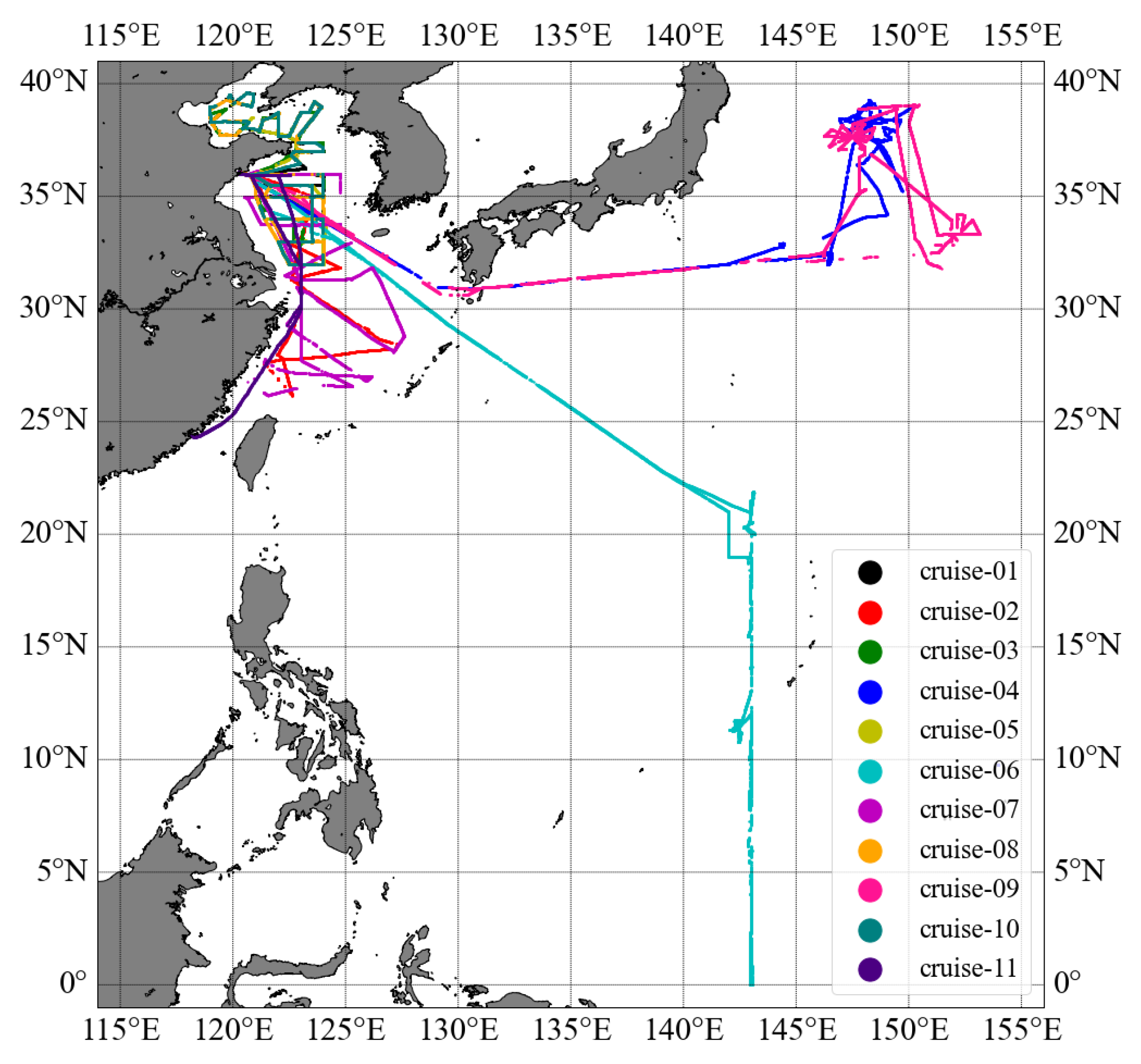
2.1. Shipboard Measurements

All the data used in this study were collected by instruments onboard Ocean University of China’s research vessel Dong Fang Hong II. The measurements comprised 11 cruises ranging from August 2015 to October 2018. As shown in Figure 1, the cruise tracks mainly cover regions in the Northwest Pacific Ocean, including eight cruises in the China Seas and their adjacent waters, two in the waters east of Japan (Cruise–04, Cruise–09), and one that headed south to the Equator (Cruise–06). The time periods and ranges of latitudes and longitudes for each cruise are shown in

Table 1. Cruise information including start and end date, ranges of latitudes, longitudes and $SS{T}_{skin}$ measurements.

Cruise Number	Start Date	End Date	Latitude	Longitude	$\mathit{S}\mathit{S}{\mathit{T}}_{\mathit{s}\mathit{k}\mathit{i}\mathit{n}}\left(\mathbf{K}\right)$
01	16 Aug. 2015	07 Sep. 2015	31.99°N–39.62°N	118.94°E–124.03°E	294.1–301.2
02	17 Oct. 2015	04 Nov. 2015	26.17°N–36.1°N	120.25°E–127.29°E	290.7–299.7
03	13 Jan. 2016	01 Feb. 2016	31.98°N–39°N	118.95°E–124.01°E	271.1–285.1
04	20 Mar. 2016	26 Apr. 2016	30.9°N–39.17°N	120.52°E–150.09°E	275.3–297.0
05	27 Dec. 2016	17 Jan. 2017	31.98°N–39.62°N	118.97°E–124.13°E	276.2–287.7
06	31 Jan. 2017	15 Mar. 2017	0°–36.1°N	120.25°E–143.17°E	277.2–303.8
07	22 Mar. 2017	15 Apr. 2017	26.17°N–36.14°N	120.26°E–127.6°E	278.5–297.8
08	17 Dec. 2017	11 Jan. 2018	31.97°N–39.62°N	118.94°E–124.02°E	274.5–287.0
09	03 May. 2018	22 Jun. 2018	30.62°N–39.08N	120.26°E–153.14°E	283.2–300.2
10	20 Jul. 2018	10 Aug. 2018	31.99°N–39.62°N	118.95°E–123.98°E	294.3–306.5
11	17 Sep. 2018	31 Oct. 2018	24.32°N–36.11°N	118.12°E–123.04°E	288.5–300.2

, every cruise lasted for half a month to one and a half.

The infrared sea surface temperature autonomous radiometer (ISAR) provided the $SS{T}_{skin}$ measurements. ISAR is a self-calibrating radiometer that has a spectral range from 9.6 to 11.5 μm and is capable of measuring $SS{T}_{skin}$ at depth of around 10 μm with accuracy of ±0.1 K [19]. The ISAR-5C was deployed on the port side of the top deck at height of about 13 m and measured the sea surface and sky with view angles of 135° and 45° from zenith. Sea surface emissivity (SSE) is the key variable in the retrieval of $SS{T}_{skin}$. SSE varies with view angles, wavelengths, wind speeds, etc. [20,21,22]. Errors of SSE at large view angles and high wind speed conditions will introduce large uncertainties in $SS{T}_{skin}$ measurements [23]. A constant value of 0.9871 for SSE was used in this ISAR-5C $SS{T}_{skin}$ algorithm considering the broad-band spectral response and 135° viewing zenith angle. The radiometer was calibrated before and after every cruise using an external blackbody that could be traced to the National Physical Laboratory’s (NPL) radiometric standards from the international comparison campaign, named fiducial reference measurements for surface temperatures derived by satellite (FRM4STS) [24]. The calibration results of both pre- and post-cruise showed good agreement with the ±0.1 K accuracy of ISAR-5C. The measurements which were collected near ports were eliminated since the target of the radiometer might not be the sea, and the true sea surface might be contaminated by complicated factors. The $SS{T}_{skin}$ was measured every 4 to 5 min and had a temperature range from around 271.1 K to 306.5 K throughout all the cruises. The ranges of $SS{T}_{skin}$ measurements for each cruise are shown in Table 1. The largest range of $SS{T}_{skin}$ occurred in Cruise–06, which ranged from 277.2 K to 303.8 K.

The $SS{T}_{depth}$ was measured by a Sea Bird SBE 48 hull temperature sensor that was deployed on the same port side of the ship’s hull at around 4 m depth below the waterline. Since the measured depth of SBE 48 is about 4 m, the $SS{T}_{depth}$ cannot be considered equivalent to the foundation SST, this will lead to an underestimation of the diurnal warming effect [7]. The $SS{T}_{depth}$ data were collected every second. The downwelling longwave and shortwave solar radiation were measured by the Kipp & Zonen CGR4 pyrgeometer and CMP21 pyranometer, respectively. The height of solar radiation measurements was 15 m above the waterline in order to be as unobstructed as possible within their 180° field of view. The wind speed, air temperature and pressure, and relative humidity measurements were all provided by the vessel management system (VMS) on the Dong Fang Hong II. The wind speed data were measured at height of 19 m, and other meteorological sensors shared an observing platform, which was 18 m height above the sea surface. According to the VMS data description, wind speed measurements were corrected using the ship’s heading and speed information. The wind speeds were converted to the reference height of 10 m (U₁₀) using the F96 model, for which calculation details were referred to by Smith (1988) [25]. The invalid data of SBE 48, solar radiation, and meteorological sensors were eliminated. The solar radiation and meteorological measurements were averaged every minute. Figure 2 shows the distributions of the data (73,706 measurements in total) with time series in months (Figure 2a), U₁₀ (Figure 2b), and $SS{T}_{skin}$ (Figure 2c). Measurements were distributed in every month, and the maximum and minimum occurred in October and November with total measurements of 11,518 and 925, respectively. There are relatively fewer data under lower temperatures below 277 K and higher temperatures above 303 K. Most of the measurements were distributed under moderate and low wind speeds, which was 16% when U₁₀ was greater than 10 m/s.

2.2. Cool Skin and Diurnal Warming Models

2.2.1. F96 Model

Fairall et al. estimated both cool skin and diurnal warming effects using measurements from the TOGA COARE program held from 1992 to 1993 [2,26]. The F96 cool skin model followed the physical basis proposed by Saunders [1]. The net heat flux $Q_{net}$ transferred from cool skin layer to the air is given by

$$Q_{net}=Q_l+Q_s+Q_{lw}$$

(1)

where $Q_l$ is latent heat flux, $Q_s$ is sensible heat flux, and $Q_{lw}$ is net longwave flux. The cool skin $\Delta T_C$ is calculated as

$$\Delta T_C=\frac{Q_{net}\delta }{k}$$

(2)

where $\delta$ is the thickness of the cool skin, $k$ is the thermal conductivity of the water, and $\delta$ is given by

$$\delta =\frac{\lambda \nu }{{({\rho }_a/\rho )}^{1/2}{u}_{*a}}$$

(3)

where $\lambda$ is the Saunders constant; $\nu$ is the kinematic viscosity; ${\rho }_a$ and $\rho$ are the densities of air and seawater, respectively; and $u_{*a}$ is the atmospheric friction velocity. Details of the Saunders constant calculation can be found in Section 2.2 of the literature [2].

The diurnal warming effect-modeled $\Delta T_w$ in F96 is given as

$$\Delta T_w=\frac{2Q_{ac}}{\rho c_p{D}_T}$$

(4)

where $Q_{ac}$ is the integrated radiative fluxes, $c_p$ is the specific heat of seawater, and $D_T$ is the thickness of the warming layer.

The COARE v3.6 was used to model F96 cool skin and diurnal warming effect in this study. The model takes $SS{T}_{skin}$; $SS{T}_{depth}$; and meteorological data including wind speed, air temperature and pressure, relative humidity, and their measuring heights as inputs and outputs air–sea fluxes, $\Delta T_C$, $\Delta T_w$, U₁₀, etc.

2.2.2. POSH Model

Gentemann et al. refined F96 diurnal warming model and this modified model can provide temperature profiles within the warm layer, hereafter called the profiles of ocean surface heating (POSH) [15]. The POSH model changes the local time of setting to zero of accumulated heat and momentum from 0 a.m. to 6 a.m. The F96 model does not account for dissipation that causes measurements to rapidly deviate due to the lack of viscous dissipation and any heat or momentum exchanges through the base of the warm layer. The POSH model considers that the diurnal warming may persist from night to the following day when wind speeds are low, and the diurnal temperature layer is not fully eroded. A nine-band spectral parameterization was used in POSH instead of the previous three-band one, which exhibited strong absorption characteristics at all depths, particularly in shallow layers, thereby enabling improved capture of the heating profiles of shallow diurnal thermoclines. To better model the depth of radiation absorption, the effect of the subsurface solar angle was also considered. The total radiation $Q_{tot}$ within the warm layer is given by

$$Q_{tot}=1.2(1-r_{SW})Q_{SW\downarrow }{f}_w(D_T)-(Q_{lw}+Q_s+Q_l)$$

(5)

where $r_{SW}$ is the mean reflectivity of the sea surface, $Q_{SW\downarrow }$ is the downwelling shortwave radiation, and $f_w(D_T)$ is the attenuation of shortwave radiation within the warm layer [15].

The F96 model assumes that the accumulated warm layer heat only decreased through longwave radiation and sea surface turbulence fluxes and that there is no heat conduction between the warm layer and the mixed layer. However, the heat is reduced through heat conduction and turbulence mixing that passes through the bottom of the warm layer, and the momentum dissipates through viscous effects. The diurnal profile is linear-interpolated in F96 model, but the POSH model calculates it using non-linear ways at time and depth steps. The refined model is given by

$$\Delta T(z)=e^{-9.5(\frac{z}{D_T})}{}^a$$

(6)

where $a$ is the coefficient of the empirical formula related to the wind speed [15]. The POSH model takes input data such as the $SS{T}_{depth}$, wind speed, and air temperature and outputs daily diurnal warming data and the temperature profile for the warm layer.

2.2.3. ZB05 Model

Based on the one-dimensional ocean heat transfer equation, Zeng and Beljaars proposed the ZB05 model for calculating diurnal warming [14]. Given wind speed, solar radiation, and $SS{T}_{depth}$ data as input, $SS{T}_{skin}$ data are calculated through the cool skin and the diurnal warming effect. The equation of the cool skin is defined as

$$T_s-T_{-\delta }=\frac{\delta }{{\rho }_w{C}_W{K}_w}(Q+R_s{f}_s)$$

(7)

where $T_s$ is the $SS{T}_{skin}$, $\delta$ is the thickness of the cool skin layer, ${\rho }_w$ is the density of the water, $C_W$ is the specific heat of water, $K_w$ is the thermal conductivity of water, $Q$ is the net heat flux in Equation (1), $R_s$ is the shortwave solar heat flux, and $f_s$ is the fraction of solar radiation absorbed in the sublayer. As for the diurnal warming effect, the top of the warm layer corresponds to the bottom of the cool skin layer. Takaya et al. refined ZB05 model including modifications to the Monin–Obukhov similarity function for stable conditions and the mixing enhancement by Langmuir circulation [16]. The rate of temperature change within this layer is as follows:

$$\frac{𝜕(T_{-\delta }-T_{-d})}{𝜕t}=\frac{Q+R_s-R(-d)}{d{\rho }_w{c}_w\nu /(\nu +1)}-\frac{(\nu +1)k{u}_{*w}}{d{\phi }_t(d/L){(U_{*w}/U_s)}^{1/3}}(T_{-\delta }-T_{-d})$$

(8)

where $d$ is the depth of the warm layer, $T_{-d}$ is the $SS{T}_{depth}$, $\nu$ is the empirical function based on d, $k$ represents the von Karman constant and is set as 0.4, $u_{*w}$ is the friction velocity of seawater, and L represents the Monin–Obukhov length. $U_s$ is the sea surface Stokes velocity, which is set to 1 cm/s [17]. The modified stability function ${\phi }_t$ is given as

$$\begin{array}{ll}{\phi }_t(\frac{-z}{L})=1+\frac{5\frac{-z}{L}+4{(\frac{-z}{L})}^2}{1+3\frac{-z}{L}+0.25{(\frac{-z}{L})}^2}& \frac{-z}{L}\ge 0\\ {\phi }_t(\frac{-z}{L})={(1-16\frac{-z}{L})}^{-1/2}& \frac{-z}{L}<0\end{array}$$

(9)

The refined ZB05 model is used in this study, which uses measurements of $SS{T}_{depth}$, wind speed, air temperature, and solar radiation as inputs.

When comparing outputs of diurnal warming models to field observation, we used modeled diurnal warming $\Delta T_W$ and cool skin $\Delta T_C$ to correct $SS{T}_{depth}$ to $SS{T}_{skin}$. The corrected $SS{T}_{skin}$ is given as

$$SS{T}_{skin}=SS{T}_{depth}+\Delta T_W-\Delta T_C$$

(10)

where the $\Delta T_W$ is the modeled diurnal warming effect, and the $\Delta T_C$ is the F96-modeled cool skin effect used in this study [2]. The $SS{T}_{skin}$ in Equation (10) represents the simulated skin temperature using diurnal models.

3. Results and Discussion

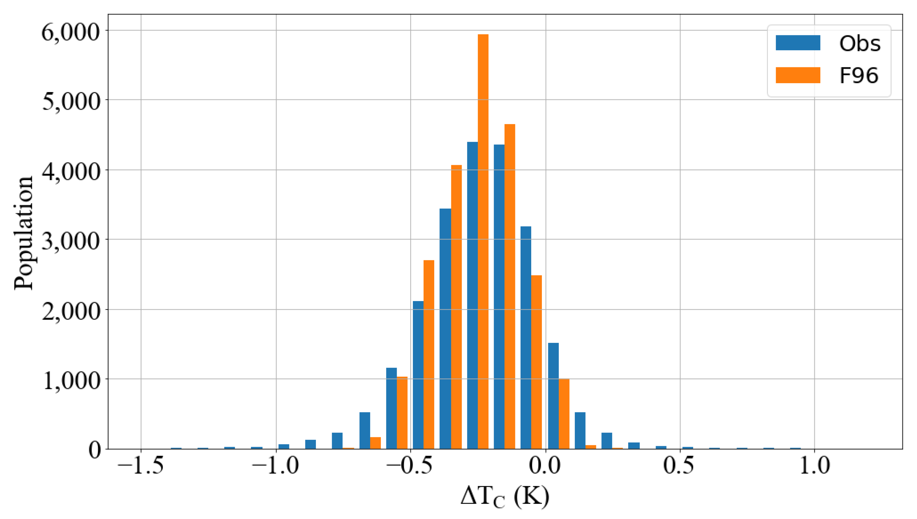
3.1. Cool Skin Effect

This section validates the F96 cool skin model using the cruises’ measurements. The $SS{T}_{depth}$ measurement depth in the study was around 4 m. To avoid the influence of the diurnal warming effect on the cool skin effect, only nighttime data with an absolute value of the solar zenith angle greater than 110° were used in the study considering less solar heating residuals from sunset to midnight [6].

The histograms of the F96-modeled cool skin and the observed (Obs) $\Delta T_C$ are shown in Figure 3.

Table 2. Statistics for the observed and F96-modeled cool skin $\Delta T_C$. “Mean” stands for the averaged value; “Mid” stands for the median value; “STD” stands for the standard deviation; “RSD” stands for the robust standard deviation; “N” is the total number of measurements.

	Mean (K)	Mid (K)	STD (K)	RSD (K)	N
Obs	−0.23	−0.22	0.22	0.19	22,085
F96	−0.25	−0.25	0.15	0.15	22,085

displays the statistics of the $\Delta T_C$, which shows a total number of 22,085 measurements. As shown in Figure 3, the F96-modeled $\Delta T_C$ were distributed between −0.7 K and 0.56 K, with 4.8% positive values and 95.2% below 0 K. The observed $\Delta T_C$ ranged from −1.44 K to 1.13 K, with a higher number of positive values, 2467 measurements, accounting for 11.2%. The mean values of the F96-modeled and observed $\Delta T_C$ were close, −0.25 K and −0.23 K, respectively. The standard deviation of the F96-modeled $\Delta T_C$ was 0.15 K, which was smaller than the 0.22 K of the observed $\Delta T_C$.

Figure 4 shows the $\Delta T_C$ as a function of the U₁₀ measurements. In previous studies on the cool skin effect, the negative mean values of the cool skin $\Delta T_C$ were larger at lower wind speeds, and the magnitudes of the $\Delta T_C$ decreased as the wind speed increased. The mean value of the $\Delta T_C$ stabilized under high wind speed conditions. However, in this study, the magnitudes of the mean values for both the F96-modeled and observed $\Delta T_C$ increased as the U₁₀ increased from 0 to 2 m/s, possibly due to the residual of the strong diurnal warming effect from sunset to midnight. Under high wind speed conditions where the U₁₀ was greater than 10 m/s, the magnitudes of the observed $\Delta T_C$ increased from −0.15 K to −0.31 K. Figure 5a shows the relationships between months and measured sea–air temperature difference, and Figure 5b shows the relationships between months and U₁₀ observation. The sea–air temperature difference had an obvious seasonal variability, which the mean value reached 3.1 K in January and reduced to around 0 K in summer. The high wind speed conditions mainly occurred from January to May, together with relatively higher sea–air temperature differences. Figure 6 shows the $\Delta T_C$ as a function of the sea–air temperature differences. The magnitudes of the observed $\Delta T_C$ increased from −0.16 K to −0.41 K when the sea–air temperature differences increased from −2 K to 7 K. The positive correlation in Figure 6 may be the main factor affecting the overestimation of the $\Delta T_C$ under high wind speeds, as the higher sea–air temperature difference results in more latent and sensible heat transfer.

The F96-modeled and observed $\Delta T_C$ as a function of the $SS{T}_{skin}$ measurements are shown in Figure 7. The relationship between the $\Delta T_C$ and $SS{T}_{skin}$ measurements is not significant in this study. The magnitudes of the observed $\Delta T_C$ decreased from −0.31 K to −0.14 K when the $SS{T}_{skin}$ increased from 290 K to 302 K, showing a negative correlation with skin temperature. It was different from the positive correlation that was proposed in previous research [4,6]. The F96-modeled $\Delta T_C$ can simulate the trends of the cool skin effect with the $SS{T}_{skin}$ well under the relatively higher measurement numbers.

3.2. Diurnal Warming Effect

The F96, POSH, and ZB05 diurnal warming models are compared with the observations in this section. Only daytime data with an absolute value of the solar zenith angle less than 90° were used in this study. The analysis in this section focuses on the relationships between the temperature differences (modeled $SS{T}_{skin}$ minus observed $SS{T}_{skin}$) and factors including U₁₀, local time, and shortwave solar radiation.

Figure 8 displays the scatter plots of the observed $SS{T}_{skin}$ with F96, POSH, and ZB05-modeled $SS{T}_{skin}$. The red dashed lines display a 1:1 relationship, while the orange solid line represents the fitted lines using the least squares method.

Table 3. Statistics for the temperature differences (modeled $SS{T}_{skin}$ minus observed $SS{T}_{skin}$ ) using three diurnal warming models.

	Mean (K)	Mid (K)	STD (K)	RSD (K)	N
F96–Obs	0.00	−0.02	0.38	0.18	35,638
POSH–Obs	0.01	−0.01	0.35	0.18	35,638
ZB05–Obs	0.21	0.10	0.46	0.29	35,638

shows the statistics on the temperature differences. The total number of daytime measurements was 35,638. The average $SS{T}_{skin}$ differences between the F96 model and the observation are close to 0 K, the same for the POSH model, and the standard deviations are 0.38 K and 0.35 K, respectively. The difference between ZB05-modeled $SS{T}_{skin}$ and the observation showed a mean value of 0.21 K and a standard deviation of 0.46 K.

The difference between the model $SS{T}_{skin}$ minus the observed $SS{T}_{skin}$ as a function of U₁₀ for the results of the three models is shown in Figure 9a. The F96- and POSH-modeled differences shared a similar relationship. The mean values and standard deviations of the differences were larger at low wind speeds and decreased to be stable as U₁₀ increases. The maximum mean differences between F96 and POSH were 0.21 K and 0.17 K under a U₁₀ less than 4 m/s, respectively. As for a U₁₀ greater than 4 m/s, the mean differences were close to 0 K. The ZB05 model overestimated the differences under all wind speed conditions, and the maximum mean difference at low wind speeds was 0.44 K. The mean differences and standard deviations of the ZB05 model continuously decreased as the wind speed increased. The reason for the larger bias at low wind speeds may be that the assumption of extending the vertical temperature distribution from the sea surface to a fixed depth is inappropriate when the wind-driven mixing is weak [15,17].

Figure 9b illustrates that the mean differences between the F96 and POSH models remain within ±0.1 K as a function of the shortwave solar radiation. The POSH model had smaller mean differences compared to the F96 model within the whole range of solar radiation variation. This was mainly due to the modification of the solar shortwave radiation absorption model for the warm layer in POSH, which was changed to a nine-band exponential absorption model, resulting in better heat accumulation [15]. The ZB05 model began to show positive differences when the shortwave solar radiation was greater than 200 W/m², which continued to increase with increasing solar radiation, with a maximum average deviation of 0.9 K. The reason for this phenomenon may be that the model assumes the depth of the warm layer to be a constant value of 3 m [27].

In order to investigate the effect of the dissipation rate of the heat in the warm layer, especially in the late afternoon, we further checked the relationship between the difference and the local time. Figure 9c displays the variation in modeled differences with local time. The F96 model exhibited positive mean differences before 8 a.m. and negative mean differences until 3 p.m., after which it became positive again and reached a maximum positive difference of 0.13 K. The large positive bias of the F96 model in the late afternoon may be caused by the assumption that the warm layer does not exchange heat and momentum with the mixed layer, resulting in the accumulation of heat and momentum in the warm layer. The slow decay rate of the heat and momentum in the warm layer was set by the F96 model, which led to the overestimation of the modeled $SS{T}_{skin}$ [15]. In contrast, the mean differences in the POSH model were close to zero at all times, with the maximum value of 0.05 K at 3 p.m. The faster decay rate of the heat and momentum in POSH avoided the overestimation of the diurnal warming effect. The ZB05 model showed positive differences throughout almost the entire day due to the overestimation under solar radiation greater than 300 W/m². The maximum mean difference was 0.46 K, which occurred at 12 a.m. In addition, the ZB05 model had a slight negative bias in the late afternoon, mainly due to the rapid dissipation rate of the heat in the warm layer, though in an actual situation the residual heat may remain in the upper ocean layer after sunset, sometimes persisting until midnight [14].

In order to further explore the performance of the three diurnal warming models, data from 46 days that had significant diurnal warming effects were selected. Selected measurements of diurnal warming as functions of local time, wind speed, and solar radiation are shown in Figure 10. The maximum observed diurnal warming effect value was 3.3 K, as shown in Figure 10a. The observed diurnal warming effect began to appear at 7 a.m. and reached its peak value at 1–2 p.m. Figure 10b illustrates that larger diurnal warming effects were observed under low wind speed conditions, which then decreased due to the mixing of the upper ocean caused by stronger winds. The relationship between the diurnal warming effect and shortwave solar radiation indicates that stronger solar radiation results in an increase in the effect amplitude.

Figure 11 presents the relationships between the mean temperature differences in the three models and the variables of U₁₀, shortwave solar radiation, and local time. The F96 model showed a maximum positive mean difference of 0.26 K and a maximum negative mean difference of −0.06 K under a U₁₀ less than 7 m/s. The POSH model had the largest positive mean difference of 0.05 K at the lowest wind speed, which overall showed negative differences as the wind speed increased, with a maximum negative mean difference of −0.10 K under a U₁₀ less than 7 m/s. When the wind speed was greater than 5 m/s, the F96- and POSH-modeled mean differences shared similar patterns. The ZB05 model overestimated differences compared to the F96 and POSH models under a U₁₀ less than 9 m/s. The ZB05 model decreased when the wind speed increased and had a maximum positive difference of 0.41 K.

The F96 model had the maximum positive mean difference of 0.20 K under the lowest shortwave solar radiation (<50 W/m²), as shown in Figure 11b. As the solar radiation increased, the differences decreased and turned into negative values at around 550 W/m². The maximum negative difference was −0.24 K when the solar radiation reached about 1000 W/m². The POSH model performed well with solar radiation less than 700 W/m² and showed increasing negative differences, down to −0.23 K at 800–850 W/m². The ZB05 model showed overall positive mean differences, with a maximum value of 1.2 K at 900~950 W/m².

As shown in Figure 11c, the F96 model underestimated the diurnal warming effect during the local time period of 9 a.m. to 3 p.m., which was basically the period that the peak diurnal warming effect occurred. The maximum negative difference was −0.17 K at 1–2 p.m. The F96 model showed a positive difference, with a maximum value of 0.5 K during the dissipation phase of the diurnal warming effect at dusk. The ZB05 model generally overestimated the differences, with a maximum value of 0.67 K from 12 a.m. to 1 p.m. In addition, there was a negative mean difference of −0.18 K at the time period of 6 p.m. to 7 p.m. The POSH model was the closest one to the observed values, with a maximum mean difference of −0.18 K from 10 to 11 a.m. The trend of the relationships in Figure 9 and Figure 11 showed some discrepancies in comparison with Luo et al. (2022), which evaluated ZB05 and F96 models using measurements in the Caribbean region [7]. The F96 modeled difference had positive biases of 0.1 K to 0.2 K at solar radiation ranged from 0 to 800 w/m2, and it was close to 0 K in this study. The models often use some average or default values, which may result in discrepancies when applying in different regions.

4. Conclusions

Simulating and measuring the effects of cool skin and diurnal warming are important parts of studying SST. In this study, shipboard measurements including $SS{T}_{skin}$, $SS{T}_{depth}$, longwave and shortwave solar radiation, wind speed, and other auxiliary data were utilized to validate modeled skin effects. The measurements were collected in the Northwest Pacific Ocean from August 2015 to October 2018.

The study evaluated three models, namely, F96, POSH, and ZB05. The F96 cool skin model demonstrated a good performance in simulating the $\Delta T_C$, in comparison to the measurements. Moreover, the F96 model could capture the relationships between the cool skin effect and wind speed, $SS{T}_{skin}$, as well as the sea–air temperature difference. There was an overestimation of cool skin $\Delta T_C$ under high wind speeds greater than 10 m/s, the measurements mainly occurred in winter and spring together with higher sea–air temperature differences. A significant positive correlation between the sea–air temperature difference and the amplitude of the cool skin effect was observed in this study, which may cause the overestimation of cool skin under a high wind speed.

The F96 and POSH models simulated the diurnal warming effect with temperature differences approaching 0 K, while the mean difference of the ZB05 model was 0.21 K. The wind speed, shortwave solar radiation, and local time are important factors affecting the diurnal warming effect. The validation results revealed that the F96 and POSH models performed well compared to the ZB05 model, except that the F96 model overestimated the difference in the late afternoon in local time. Additionally, data that exhibited a clear diurnal warming effect were selected to validate the models, and the POSH model was the closest one to the observation. More models will be validated in future work. The regional measurements and the validation of the cool skin and diurnal warming effects in this study could serve as a reference for the thermal skin effects, air–sea interaction, and upper ocean gradient research. In particular, the process of satellite SST inversion using buoy $SS{T}_{depth}$ data should be corrected by the cool skin and diurnal warming models, as well as the validation. The discrepancies of different models and their variabilities related to the factors according to the findings of this study should be taken care of and discussed.

References

1. Saunders, P.M. The temperature at the ocean-air interface. J. Atmos. Sci. 1967, 24, 269–273. [Google Scholar] [CrossRef]
2. Fairall, C.W.; Bradley, E.F.; Godfrey, J.S.; Wick, G.A.; Edson, J.B.; Young, G.S. Cool-skin and warm-layer effects on sea surface temperature. J. Geophys. Res. 1996, 101, 1295–1308. [Google Scholar] [CrossRef]
3. Donlon, C.J.; Minnett, P.J.; Gentemann, C.L.; Nightingale, T.; Barton, I.; Ward, B.; Murray, J. Toward Improved Validation of Satellite Sea Surface Skin Temperature Measurements for Climate Research. J. Clim. 2002, 14, 353–369. [Google Scholar] [CrossRef]
4. Minnett, P.J.; Smith, M.; Ward, B. Measurements of the oceanic thermal skin effect. Deep Sea Res. Part II 2011, 58, 861–868. [Google Scholar] [CrossRef]
5. Alappattu, D.P.; Wang, Q.; Yamaguchi, R.; Lind, R.J.; Reynolds, M.; Christman, A.J. Warm layer and cool skin corrections for bulk water temperature measurements for air-sea interaction studies. J. Geophys. Res. Ocean. 2017, 122, 6470–6481. [Google Scholar] [CrossRef]
6. Zhang, H.F.; Beggs, H.; Ignatov, A.; Babanin, A.V. Nighttime Cool Skin Effect Observed from Infrared SST Autonomous Radiometer (ISAR) and Depth Temperatures. J. Atmos. Ocean. Technol. 2020, 37, 33–46. [Google Scholar] [CrossRef]
7. Luo, B.K.; Minnett, P.J.; Szczodrak, M.; Akella, S. Regional and Seasonal Variability of the Oceanic Thermal Skin Effect. J. Geophys. Res. Ocean. 2022, 127, e2022JC018465. [Google Scholar] [CrossRef]
8. Tu, C.Y.; Tsuang, B.J. Cool-skin simulation by a one-column ocean model. Geophys. Res. Lett. 2005, 32, L22602. [Google Scholar] [CrossRef] [Green Version]
9. Jia, C.; Minnett, P.J.; Luo, B.K. Significant diurnal warming events observed by Saildrone at high latitudes. J. Geophys. Res. Ocean. 2023, 128, e2022JC019368. [Google Scholar] [CrossRef]
10. Soloviev, A.; Lukas, R. Observation of large diurnal warming events in the near-surface layer of the western equatorial Pacific warm pool. Deep Sea Res. Part I 1997, 44, 1055–1076. [Google Scholar] [CrossRef] [Green Version]
11. Ward, B. Near-surface ocean temperature. J. Geophys. Res. Ocean. 2006, 111, C02004. [Google Scholar] [CrossRef] [Green Version]
12. Gentemann, C.L.; Minnett, P.J. Radiometric measurements of ocean surface thermal variability. J. Geophys. Res. Ocean. 2008, 113, C08017. [Google Scholar] [CrossRef] [Green Version]
13. Price, J.F.; Weller, R.A.; Pinkel, R. Diurnal cycling: Observations and models of the upper ocean response to diurnal heating, cooling, and wind mixing. J. Geophys. Res. 1986, 91, 8411–8427. [Google Scholar] [CrossRef] [Green Version]
14. Zeng, X.B.; Beljaars, A. A prognostic scheme of sea surface skin temperature for modeling and data assimilation. Geophys. Res. Lett. 2005, 32, L14605. [Google Scholar] [CrossRef] [Green Version]
15. Gentemann, C.L.; Minnett, P.J.; Ward, B. Profiles of ocean surface heating (POSH): A new model of upper ocean diurnal warming. J. Geophys. Res. Ocean. 2009, 114, C07017. [Google Scholar] [CrossRef] [Green Version]
16. Takaya, Y.; Bidlot, J.R.; Beljaars, A.C.M.; Janssen, P. Refinements to a prognostic scheme of skin sea surface temperature. J. Geophys. Res. Ocean. 2010, 115, C06009. [Google Scholar] [CrossRef] [Green Version]
17. Akella, S.; Todling, R.; Suarez, M. Assimilation for skin SST in the NASA GEOS atmospheric data assimilation system. Q. J. R. Meteorol. Soc. 2017, 143, 1032–1046. [Google Scholar] [CrossRef] [Green Version]
18. Zhang, R.W.; Zhou, F.H.; Wang, X.; Wang, D.X.; Gulev, S.K. Cool Skin Effect and its Impact on the Computation of the Latent Heat Flux in the South China Sea. J. Geophys. Res. Ocean. 2021, 126, 2020JC016498. [Google Scholar] [CrossRef]
19. Donlon, C.J.; Robinson, I.S.; Reynolds, M.; Wimmer, W.; Fisher, G.; Edwards, R.; Nightingale, T.J. An infrared sea surface temperature autonomous radiometer (ISAR) for deployment aboard volunteer observing ships (VOS). J. Atmos. Ocean. Technol. 2008, 25, 93–113. [Google Scholar] [CrossRef]
20. Masuda, K.; Takashima, T.; Takayama, Y. Emissivity of pure and sea waters for the model sea surface in the infrared window regions. Remote Sens. Environ. 1988, 24, 313–329. [Google Scholar] [CrossRef]
21. Wu, X.; Smith, W.L. Emissivity of rough sea surface for 8–13 µm: Modeling and verification. Appl. Opt. 1997, 36, 2609–2619. [Google Scholar] [CrossRef] [PubMed]
22. Niclòs, R.; Caselles, V.; Valor, E.; Coll, C.; Sanchez, J.M. A simple equation for determining sea surface emissivity in the 3–15 µm region. Int. J. Remote Sens. 2009, 30, 1603–1619. [Google Scholar] [CrossRef]
23. Wimmer, W.; Robinson, I.S. The ISAR instrument uncertainty model. J. Atmos. Ocean. Technol. 2016, 33, 2415–2433. [Google Scholar] [CrossRef]
24. Theocharous, E.; Fox, N.P.; Barker-Snook, I.; Niclos, R.; Santos, V.G.; Minnett, P.J.; Gottsche, F.M.; Poutier, L.; Morgan, N.; Nightingale, T.; et al. The 2016 CEOS Infrared Radiometer Comparison: Part II: Laboratory Comparison of Radiation Thermometers. J. Atmos. Ocean. Technol. 2019, 36, 1079–1092. [Google Scholar] [CrossRef] [Green Version]
25. Wu, J. On the cool skin of the ocean. Bound. Layer Meteorol. 1985, 31, 203–207. [Google Scholar] [CrossRef]
26. Fairall, C.W.; Bradley, E.F.; Hare, J.E.; Grachev, A.A.; Edson, J.B. Bulk parameterization of air-sea fluxes: Updates and verification for the COARE algorithm. J. Clim. 2003, 16, 571–591. [Google Scholar] [CrossRef]
27. Bellenger, H.; Duvel, J.P. An Analysis of Tropical Ocean Diurnal Warm Layers. J. Clim. 2009, 22, 3629–3646. [Google Scholar] [CrossRef]
Figure 1. Cruise tracks with cruise numbers used in this study.
Remotesensing 15 03814 g001
Figure 2. Distributions of measurements in this study: (a) distributions with times in months; (b) distributions with U10; (c) distributions with S S T s k i n .
Remotesensing 15 03814 g002
Figure 3. The histograms of the F96-modeled cool skin and the observed (Obs) Δ T C .
Remotesensing 15 03814 g003
Figure 4. Δ T C as a function of the U10 measurements. The lines represent the mean values of the Δ T C measurements (red) and the F96 model (blue), with intervals of 1 m/s. The error bars represent the standard deviations. The bars display the populations within every interval.
Remotesensing 15 03814 g004
Figure 5. Relationships between months and measured (a) sea–air temperature difference; (b) U10 measurements. The lines represent the mean values of the measurements (red), with intervals of one month. The error bars represent the standard deviations. The bars display the populations within every interval.
Remotesensing 15 03814 g005
Figure 6. Δ T C as a function of the sea–air temperature difference measurements. The lines represent the mean values of the Δ T C measurements (red) and the F96 model (blue), with intervals of 1 K. The error bars represent the standard deviations. The bars display the populations within every interval.
Remotesensing 15 03814 g006
Figure 7. Δ T C as a function of the S S T s k i n measurements. The lines represent the mean values of the Δ T C measurements (red) and the F96 model (blue), with intervals of 1 K. The error bars represent the standard deviations. The bars display the populations within every interval.
Remotesensing 15 03814 g007
Figure 8. Scatter plots of the observed S S T s k i n with (a) F96-, (b) POSH-, and (c) ZB05-modeled S S T s k i n .
Remotesensing 15 03814 g008
Figure 9. The temperature differences (modeled S S T s k i n minus observed S S T s k i n ) as a function of (a) U10 measurements; (b) shortwave solar radiation measurements; (c) local time. The lines represent the mean temperature differences between the F96 model (red), the POSH model (blue), and the ZB05 model (green). The error bars represent the standard deviations. The bars display the populations within every interval.
Remotesensing 15 03814 g009
Figure 10. The selected measurements of diurnal warming as functions of (a) local time, (b) U10 measurements, and (c) shortwave solar radiation. The lines represent the observed bin-averaged diurnal warming amplitude. The error bars represent the standard deviations.
Remotesensing 15 03814 g010aRemotesensing 15 03814 g010b
Figure 11. The temperature differences (modeled S S T s k i n minus observed S S T s k i n ) in selected 46 days’ data as a function of (a) U10 measurements; (b) shortwave solar radiation measurements; (c) local time. The lines represent the mean temperature differences between the F96 model (red), the POSH model (blue), and the ZB05 model (green). The error bars represent the standard deviations. The bars display the populations within every interval.
Remotesensing 15 03814 g011