Technical Note

Gluing Atmospheric Lidar Signals Based on an Improved Gray Wolf Optimizer

1
Key Laboratory of Optoelectronic Information Science and Technology (Ministry of Education), School of Precision Instruments and Opto-Electronic Engineering, Tianjin University, Tianjin 300072, China
2
School of Marine Science and Technology, Tianjin University, Tianjin 300072, China
*
Author to whom correspondence should be addressed.
Remote Sens. 2023, 15(15), 3812; https://doi.org/10.3390/rs15153812
Submission received: 30 June 2023 / Revised: 26 July 2023 / Accepted: 30 July 2023 / Published: 31 July 2023

Abstract

:
Lidar is important active remote sensing equipment in the field of atmospheric environment detection. However, the detection range of lidar is severely limited by the dynamic range of photodetectors. To solve this problem, atmospheric lidars are often equipped with two or more channels to receive signals from different altitude ranges, where gluing the multi-channel echo signals becomes a key issue for accurate data inversion. In this paper, a multi-channel signal gluing algorithm based on the Improved Gray Wolf Optimizer (IGWO) and Neighborhood Rough Set (NRS), named IGWO-RSD, is proposed. The fitness function F is formed by three objective functions: correlation coefficient R, regression stability coefficient S and mean fit deviation D. All three objective functions are obtained from the data itself and do not rely on prior information. The weights of the objective functions R, S and D are pre-trained by NRS, and IGWO is used to optimize the fitness function F. With ground-based aerosol lidar data, all-day signal gluing experiments are performed, where IGWO-RSD demonstrates obvious advantages in stability, accuracy and applicability in lidar signal processing compared with NRSWNSGA-II.

Graphical Abstract

1. Introduction

Lidar is widely used in the field of atmospheric remote sensing due to its high spatial and temporal resolution, high accuracy and ability for continuous real-time monitoring. However, in medium- and long-range detection of atmospheric environments, the echo-signal intensity can cover more than six orders of magnitude, which is beyond the linear responding range of the state-of-the-art single-photon detectors. To overcome this problem, atmospheric lidar systems typically employ multi channels to collect signals from different height ranges.
There are two main multi-channel structures. The first one has receiving telescopes of different apertures or lasers at different wavelengths [1,2], while the second one separates signals of different intensities in the receiving system using optical or electrical methods [3,4,5,6]. Different detectors working in analog-to-digital mode (AD) and photon counting mode (PC) can be used to collect data from low- and high-altitude channels, respectively. The major concern of the multi-channel structure is to accurately obtain high-dynamic-range echo-signal profiles within the linear ranges of the detectors.
The echo signal of the multi-channel lidar must be glued using appropriate algorithms before the retrieving process. For this purpose, linear regression should be established through a certain gluing region of the signals to obtain the ‘‘glue coefficients’’ and then to match the AD and PC data. The current research focus is to find the optimal gluing region, mainly including three methods: strength constraint, height constraint and constraint based on certain evaluation indicators. The strength constraint refers to the upper limit of the fitting signal strength determined by the nonlinearity of the near-field channels and the lower limit of the fitting signal strength determined by the signal-to-noise ratio of the far-field channels [7,8], which can preliminarily determine the gluing region. However, Zhang et al. found that as the correlation of the dual-channel data decreases [8], the fitting results become unstable. D’Amico et al. employed a correlation coefficient and a regression stability coefficient as evaluation indicators, by gradually reducing the height range with a fixed step [9]. Huang et al. used fitting regression coefficients and gluing deviation per kilometer as evaluation indicators [10,11], and performed fixed-step traversal on the given height range based on empirical values. Both works provided relatively reliable gluing regions, but it should be noted that iteration with a fixed step size is mechanical in the algorithm, limiting the ability to search for the optimal gluing region. In addition, gluing methods based on the lamp mapping technique, statistical principles and spatiotemporal variance have been proposed [12,13,14], but they are very complex to operate or have poor applicability.
Duan et al. proposed an algorithm based on the Non-dominated Sorting Genetic Algorithm II (NSGA-II) and Neighborhood Rough Set (NRS) to obtain the optimal solution in the randomly generated initial gluing region [15], named NRSWNSGA-II. Meanwhile, the correlation coefficient R, regression stability coefficient S and standard gain ratio deviation T were selected as objective functions, which exhibited better gluing stability and accuracy than the other methods.
NRSWNSGA-II does have good performance; however, it still can be improved in terms of its objective function, solving ability and the final gluing method. In this paper, the Improved Gray Wolf Optimizer (IGWO) is proposed by using R, S and the mean fit deviation D as objective functions, which is abbreviated as IGWO-RSD. Here, D rather than T is adopted, as the indicator improves the algorithm ability in handling strong background signals, eliminates the dependency of gluing algorithms on prior information and extends the applicability of the algorithm. IGWO also improves the solution accuracy and convergence speed compared with NSGA-II. Moreover, substituting segmented gluing for point gluing ensures the smoothness of the echo-photon profile and minimizes the distortion of the original data.

2. Methods

2.1. General Idea

This paper mainly discusses data gluing of dual-channel atmospheric lidar. An optimization algorithm named IGWO-RSD is proposed to solve the gluing region and gluing coefficient corresponding to the optimal value of the objective function. The gluing coefficient G consists of the fitting slope K and intercept b, which is obtained by fitting the dual-channel data of the gluing region, shown as
N f i t = K N + b
where N is the original echo signal and Nfit is the fitted signal. The IGWO-RSD algorithm is composed of an optimization algorithm based on IGWO and a weight training algorithm based on NRS. The objective function F is defined by three parameters, the fit correlation coefficient R, the regression stability coefficient S and the mean fit deviation D. The overall process of IGWO-RSD is shown in Figure 1.
All lidar signal samples need to be preprocessed before the gluing algorithm, which mainly contains background subtraction, saturation correction of the detectors and other corrections required for lidar systems. The details of the preprocessing can be found in [9].
The samples are divided into two parts. One is the training set to obtain the weights of the objective functions and the other is the testing set to evaluate the gluing effect. NRS is used to weigh the objective functions R, S and D of the training set to obtain their weights α1, α2 and α3. Then, a composite fitness function F is defined. Next, the lidar data to be glued are optimized by IGWO to find the optimal gluing region corresponding to the optimal value of F. Thereupon, the gluing of the dual-channel data is completed.

2.2. Improved Gray Wolf Optimizer (IGWO)

The optimization aims to determine the optimal value of the decision variable by iterating the algorithm to obtain the maximum or minimum objective function under certain constraints. Usually, seeking the absolute optimal solution to optimization problems is time-consuming and costly, and optimization algorithms are required to approximate the optimal solution in a reasonable time, which has been widely used in many complex scientific and engineering fields. The Gray Wolf Optimizer (GWO) was proposed by Mirjalili et al. in 2013 [16]. As a meta-heuristic optimization algorithm, it has the advantages of simplicity, flexibility, free from inference and fast convergence. However, the GWO has problems such as a lack of population diversity, imbalanced exploitation and exploration and premature convergence. In 2020, the IGWO was put forward by Nadimi-Shahraki et al. [17], which performs better in balancing global and local searches and solves the problem of the GWO easily falling into local optima.

2.2.1. Initial Gluing Region and Fitness Function

In the IGWO, each feasible solution in the gluing region is considered a wolf, and all wolves are generated from an initial gluing region [z0, z1]. z0 represents the lowermost position of the initial gluing region, which is generally the lowest altitude in the near-field channel where nonlinearity effects caused by detector saturation can be corrected. z1 is the uppermost position of the initial gluing region, typically the highest altitude at which the signal-to-noise ratio (SNR) of the far-field channel signal is guaranteed (SNR ≥ 10). The SNR of the far-field signal above z1 is too low for atmospheric parameter inversion. The SNR is defined as
S N R = N f a r N b g N f a r
where Nfar is the far-field signal and Nbg is the background noise.
The fitness function is an evaluation index for selecting the best individual in the wolf pack, and selecting an appropriate fitness function for a specific problem is the key to obtaining the optimal solution. To obtain the optimal gluing region, three objective functions R, S and D are selected to form the fitness function F, expressed as
F = α 1 R + α 2 S + α 3 D
where the weights of three objective functions α1, α2 and α3 are determined by the weight training algorithm based on NRS, which is introduced in Section 2.3.
R is the correlation coefficient of the linear-least-squares fit between the near- and the far-field signals. The range for R is [0, 1], and a higher R indicates stronger correlations between the dual-channel signals. If the value of R is less than 0.9, the dual-channel signals are not linearly correlated. The expression of R is given by Equation (4), where Nnear and Nfar are the near- and far-field signals.
R = j ( N i j n e a r N j n e a r ¯ ) ( N i j f a r N j f a r ¯ ) j ( N i j n e a r N j n e a r ¯ ) 2 j ( N i j f a r N j f a r ¯ ) 2
If the gluing region is large, there could be a difference between the first and the second half of the gluing region. The regression stability coefficient S was defined through regression analysis in [9]. The gluing region is divided into two equal sub-regions named I1 and I2, where solving each region using Equations (5)–(7) and performing the linear-least-squares fit on the dual-channel signals provide the fitting slopes K1, K2 and residuals Re1, Re2. The corresponding fitting slopes k1 and k2 can be obtained by the linear-least-squares fit between Re and range z, as shown in Equation (7).
N i n e a r = K N i f a r
R e i = K i N i f a r N i n e a r
R e i = k i z ( i = 1 , 2 )
The definition of S is given as follows,
S = | k 1 k 2 | Δ k 1 2 + Δ k 2 2
where Δk1 and Δk2 are the standard deviations of the fitting slopes k1, k2. The larger the S, the more unstable the results of the regression analysis of the two regions. When S is increased to 1, the agreement probability between the dual-channel signals is only 32% [18].
D is defined as the average deviation between the near-field signal (Nnear) and the fitted far-field signal (Nfar_fit), as given by Equation (9). A smaller D indicates that the deviation between dual-channel signals is larger. The gluing coefficients in the i-th gluing region [z0i, z1i] are obtained by the linear-least-squares fit between the dual-channel signals. Nfar_fit is obtained through multiplying Nfar by the gluing coefficients, as shown in Equation (1). D is obtained by calculating the average deviation of Nnear and Nfar_fit for each bin within the entire initial gluing region [z0, z1].
D = | j ( N j n e a r N j f a r _ f i t ) N j n e a r Bin num |
where Binnum is the number of bins in [z0, z1], and Njnear represents the Nnear in the j-th bin.
Ref. [15] selected R, S and T as the objective functions, where T is the standard gain ratio deviation, expressed as
T = | K i K 0 | K 0
where Ki is the fitting slope of the dual-channel signals of the i-th data, K0 is the standard gain ratio, which is prior information given by the lidar system, but it is difficult to give an accurate value.
It should be noted all of the objective functions, R, S and D, come from the signal itself, while T relies on prior information K0. The third section will show that introducing incorrect prior information (inaccurate K0) into the gluing algorithm can lead to significant errors. Given that, D is used to replace T as the third objective function in this paper. In this way, no additional error is introduced because all of the objective functions only rely on the characteristics of the signal itself rather than any other prior information.

2.2.2. Fundamentals

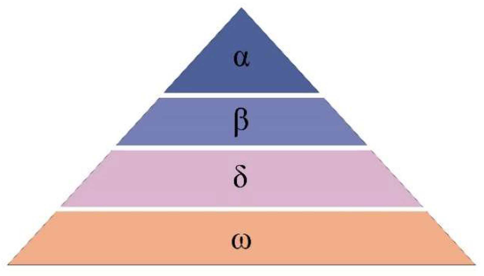
The basic principle of the IGWO algorithm is briefly introduced here, and the specific implementation of the algorithm can be found in [16,17]. The gray wolf is a pack animal with a very strict internal hierarchy, and the IGWO searches for the optimal solution by simulating the social hierarchy and hunting behavior of gray wolves. The hierarchy of wolves can be represented as shown by Figure 2, where all wolves are classified into four categories: α, β, δ and ω. α, βand δ are leaders who can guide the other ordinary members, named ω, toward promising areas to find global optimal solutions.
The hunting behavior of wolves consists of three steps: encircling, hunting and attacking the prey, and the IGWO’s iterative process of finding the optimal solution is similar. The process of wolves encircling their prey can be described by Equation (11), where Xp is the location of the target, X(i) is the position vector of the i-th iteration of gray wolves, A and C are coefficient vectors defined by Equation (13) and r1, r2 are random factors in [0, 1].
D = | C × X p X ( i ) |
X ( i + 1 ) = X p ( i ) A × D
A = 2 × A × r 1 a ( i )
C = 2 × r 2
where a is defined by
a ( i ) = 2 ( 2 × i ) / M a x I t e r
MaxIter in Equation (15) represents the maximum set number of program iterations. a linearly decreases from 2 to 0 when the number of iterations is increased, and the global and local search capabilities of the algorithm can be balanced by changing the decrease method into nonlinear functions.
For each wolf, the distances Dα, D𝛽 and Dδ from α, 𝛽 and δ were solved from Equation (11). Then, the step and direction of ω moving towards α, β and δ are defined by Equation (12), that is X1(i), X2(i), X3(i), and Equation (16) represents the final position of ω after one iteration.
X G W O ( i + 1 ) = X 1 ( i ) + X 2 ( i ) + X 3 ( i ) 3
It is found that the GWO algorithm tends to prematurely converge to a local optimum when attempting to solve the problem of gluing atmospheric lidar signals. In the decision space, the fitness function F consists of three objective functions with different complex distributions. The complex fitness function leads to more local optimal solutions, so this problem requires a higher global search capability of the algorithm. The IGWO, which is described in [17], presents a dimension learning-based hunting (DLH) search strategy that increases population diversity, thereby improving the global search capability of the algorithm. The idea of the DLH search strategy is to generate another candidate XDLH through multi-neighbor learning and random factors.
The optimal solution of each iteration of the IGWO is generated from XGWO, obtained by the GWO search strategy, and XDLH, obtained by the DLH search strategy. A better solution will be obtained by comparing their fitness values, shown as follows:
X ( i + 1 ) = X G W O ( i + 1 ) , f i t ( X G W O ) < f i t ( X D L H ) X D L H ( i + 1 ) , f i t ( X G W O ) f i t ( X D L H )

2.3. Neighborhood Rough Set (NRS)

As shown in Equation (3), the fitness function F is composed of three objective functions, R, S and D. How to determine their weights α1, α2 and α3 is critical to achieve a better gluing effect.
Here, the weight training algorithm based on the NRS [15,19,20] is used to train the samples and obtain the weights of three objective functions, R, S and D. A certain number of samples U are randomly selected and the values of R, S and D are solved in a range of heights given by empirical values. In NRS, R, S and D are condition attributes. The condition attributes of each sample are evaluated and scored according to the division criteria in Table 1, and then their scores are summed to obtain the decision attribute E.
The normalized R, S and D form the evaluation matrix A. Firstly, the radius of the neighborhood of the R, S and D is determined for each sample i, shown as
r i , j = S t d ( A ˜ j ) / λ ,     i = 1 , 2 N ,     j = 1 , 2 , 3
where N is the number of samples, j represents the three conditional attributes R, S and D, Std is the standard deviation, λ characterizes the classification accuracy of the neighborhood and λ = 3 in this paper. The set of neighborhoods δB of the condition attribute B R , S , D is
δ B ( x i ) = x k | x k U , | A k , j A i , j | r i , j
where xi is the i-th sample, xk represents the other samples in U the Euclidean distance of which to xi is less than the radius of the neighborhood of xi.
By dividing U into L equivalence classes (Y1, Y2……YL) according to the scores of the decision attribute E, the lower approximation (positive domain) to B can be found:
N B E = l = 1 L N B Y l
where NBYl is given by
N B Y l = { X i | r B ( x i ) Y l , x i U }
Then, the dependency degree of the decision attribute E on B is obtained:
γ B ( E ) = card ( N B E ) / card ( U )
where card denotes the number of elements of the set, and consequently, the attribute significance to the objective function B can be derived, expressed as
S i g ( B , E ) = γ { R , S , D } ( E ) γ { R , S , D } B ( E )
The weights of the objective function B are
α ( B ) = S i g ( B , E ) m = 1 3 S i g ( B m , E )

2.4. Final Gluing Method

The IGWO algorithm is used to optimize the fitness function F, and the optimal gluing regions and gluing coefficients G for the three objective functions R, S and D are acquired, according to which the far-field signal is fitted to obtain Nfar_fit. The whole photon profile is divided into three regions as follows
N f i n = N f a r _ f i t                                                                                   f o r         z < z 0 ω ( z ) N f a r _ f i t + ( 1 ω ( z ) ) N n e a r   f o r         z Δ z N n e a r                                                                                         f o r         z > z 1 e
For the region below z0, the fitted far-field signal (Nfar_fit) is selected, where z0 is the nadir of the near-field channel where the signal nonlinearity is correctable.
The region in Δz is processed using ω(z) to average Nfar_fit and Nnear in order to ensure the smoothness of the whole profile. ω(z) is given by
ω z = cos π z z 0 / Δ z
and Δz is expressed as
Δ z = [ z 0 , z 1 e ]
where z1e is the height determined by empirical values. For short-range lidar systems such as the aerosol lidar, it can generally be taken as 300 m or shorter [9], while for medium- and long-range lidar systems such as the Rayleigh lidar, it can be taken as 1 km–2 km [5]. The length of Δz should be as short as possible to minimize the impact of smoothing on the distortion of the raw signals for further atmospheric parameter inversion.
For the region above z1e, the signal of the near-field channel (Nnear) is selected.

3. Results

The samples for the gluing experiments were downloaded from the website of the LIDAR Group of the University of Wisconsin [21]. The samples collected by the Arctic High Spectral Resolution Lidar (AHSRL) in Korea and Singapore were adopted in this paper, which included 8300 samples. All the samples had a time resolution of 1 h and a vertical resolution of 7.5 m.
The weights of the objective functions R, S and D were obtained by the NRS algorithm using 3000 randomly selected samples for weight training. Their values are shown in Table 2. Due to the differences in the R, S and D values of different samples, the sample size in the training set should be large enough to reflect the characteristics of the overall dataset. When the sample size was greater than 1500, the weights obtained from training were basically stable. In this paper, 3000 samples were selected to form the training set.
In the IGWO, the number of grey wolves was set as 100 and the number of iterations was 70. It should be noted that we chose larger parameters in order to verify the performance of the algorithm, while smaller parameters would be feasible in practical applications.

3.1. Verification of Gluing Stability

In atmospheric lidar systems, the dual-channel signals do not have the same gain ratio at all altitudes due to cloud scattering and the saturation of photon detectors, and this is the main cause of gluing instability [12]. In [15], this problem was solved by choosing objective function T to introduce a priori information K0 in the algorithm, but additional errors would be introduced if K0 was inaccurate. In this paper, we chose D to mitigate the impact of signal distortion on the gluing results, which improved the accuracy of the algorithm.
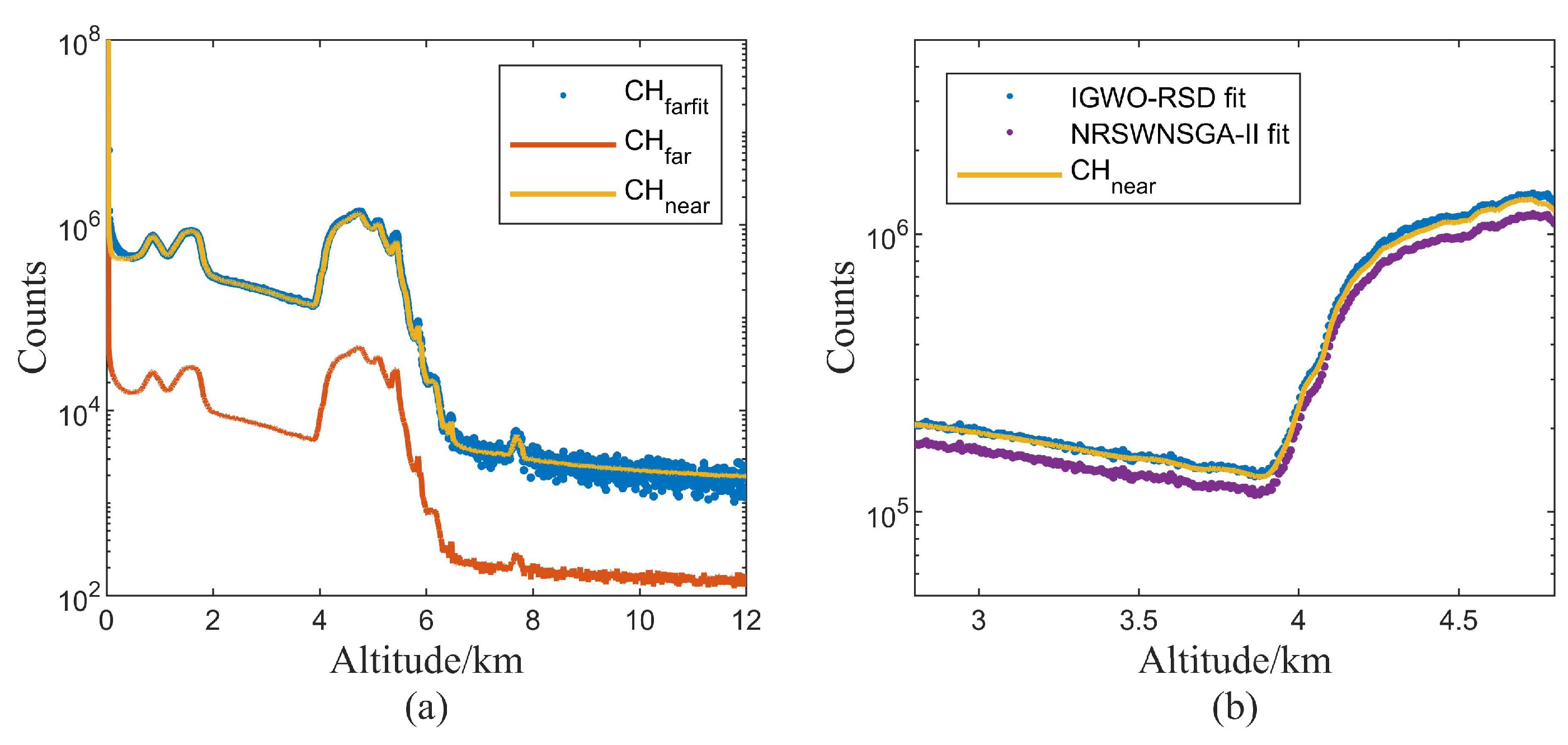
A midday (12:00 to 13:00 on 5 January 2017) sample was used to test the stability of the gluing algorithms, because the strong solar background noise leads to significant saturation at lower altitudes. The sample was glued using NRSWNSGA-II and IGWO-RSD. The gluing results are shown in Figure 3.
As shown in Figure 3a, the fitting results of the IGWO-RSD are, overall, in good agreement with using far-field signals to fit the near-field signals. The deviation in the altitude range of 0–200 m is due to the detector saturation. That the signal in the altitude range of 4–6 km signal cannot be well matched at some peaks is caused by both detector saturation and cloud scattering. In fact, the error of the near-field signals cannot be completely eliminated considering that the non-paralyzable model used in correcting saturation signals has limited applicability [9,22]. The gluing coefficients obtained by the two algorithms have differences and their fitting results are shown in Figure 3b. It can be seen that the far-field signal fitting results of the IGWO-RSD algorithm accord well to the near-field signal, while those fitted by NRSWNSGA-II demonstrate large deviations due to the influence of inaccurate K0. It indicates that the IGWO-RSD has better performance in dealing with signals with strong background noise.
In order to verify the gluing stability of the two algorithms, the gluing experiment of the midday sample was repeated 50 times using two algorithms, respectively, and the results are shown in Figure 4.
Figure 4a,b shows the distribution of the fitting slope K and counts of the near-field signal in z0, respectively. The largest deviation of K obtained by the NRSWNSGA-II algorithm from the mean value (24.5869) reaches 0.3, with a variance of 0.0259, while the deviation of the IGWO-RSD algorithm is lower than 0.1 and the variance is 0.0012, indicating that the stability of the IGWO-RSD algorithm is better than NRSWNSGA-II. Meanwhile, more than 85% of the results of IGWO-RSD converge to the same value of 28.6439, which is the global optimal solution. It should be attributed to the better search capability of the IGWO and also in part due to a better choice of the objective function D. As previously discussed, in NRSWNSGA-II, T would introduce inaccurate prior information (K0) for the gluing, resulting in an overall low fitting slope as well as degraded stability.

3.2. Comparison of Solving Capability

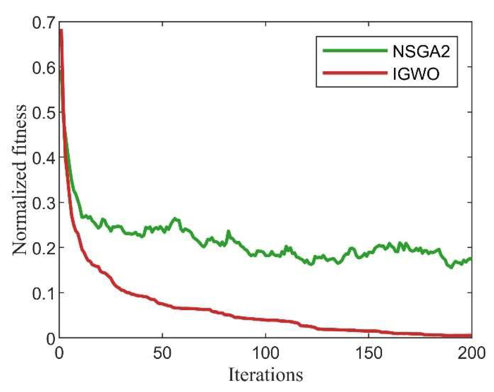
One major difference between IGWO-RSD and NRSWNSGA-II is in the selection of the optimizer, where it is the IGWO for IGWO-RSD and NSGA-II for NRSWNSGA-II. Choosing a suitable optimizer for a given problem can greatly improve the performance of the optimization algorithm. In order to verify the superiority of IGWO over NSGA-II in the problem of solving the optimal gluing region, here, we compare the convergence of two optimizers in the case of 200 iterations of the fitness value, as shown in Figure 5. The fitness function F is used to compare the solving ability of two optimizers. The horizontal and vertical axes present the number of iterations and the normalized fitness value, respectively. Since different samples converge to different fitness values, 100 samples at different times are randomly selected and each fitness value is normalized and averaged.
It can be seen in Figure 5 that the NSGA-II easily falls into the local optimum, while the IGWO has better global search capability than NSGA-II. NSGA-II falls into the local optimum after 50 iterations, while the IGWO continues to search for the global optimal solution. The fitness value obtained by NSGA-II is 20% higher than that obtained by the IGWO on average. Meanwhile, as NSGA-II is a multi-objective optimizer that focuses on solving the Pareto set of the optimal solution [23], it does not guarantee a stable decrease in the fitness function during iterating, which is not conducive to solving the gluing region with an optimal fitness value. In summary, the choice of the IGWO as the optimizer is more suitable than NSGA-II for the problem of solving the optimal gluing region of multi-channel signals of atmospheric lidar.

3.3. Full-Day Gluing Experiment

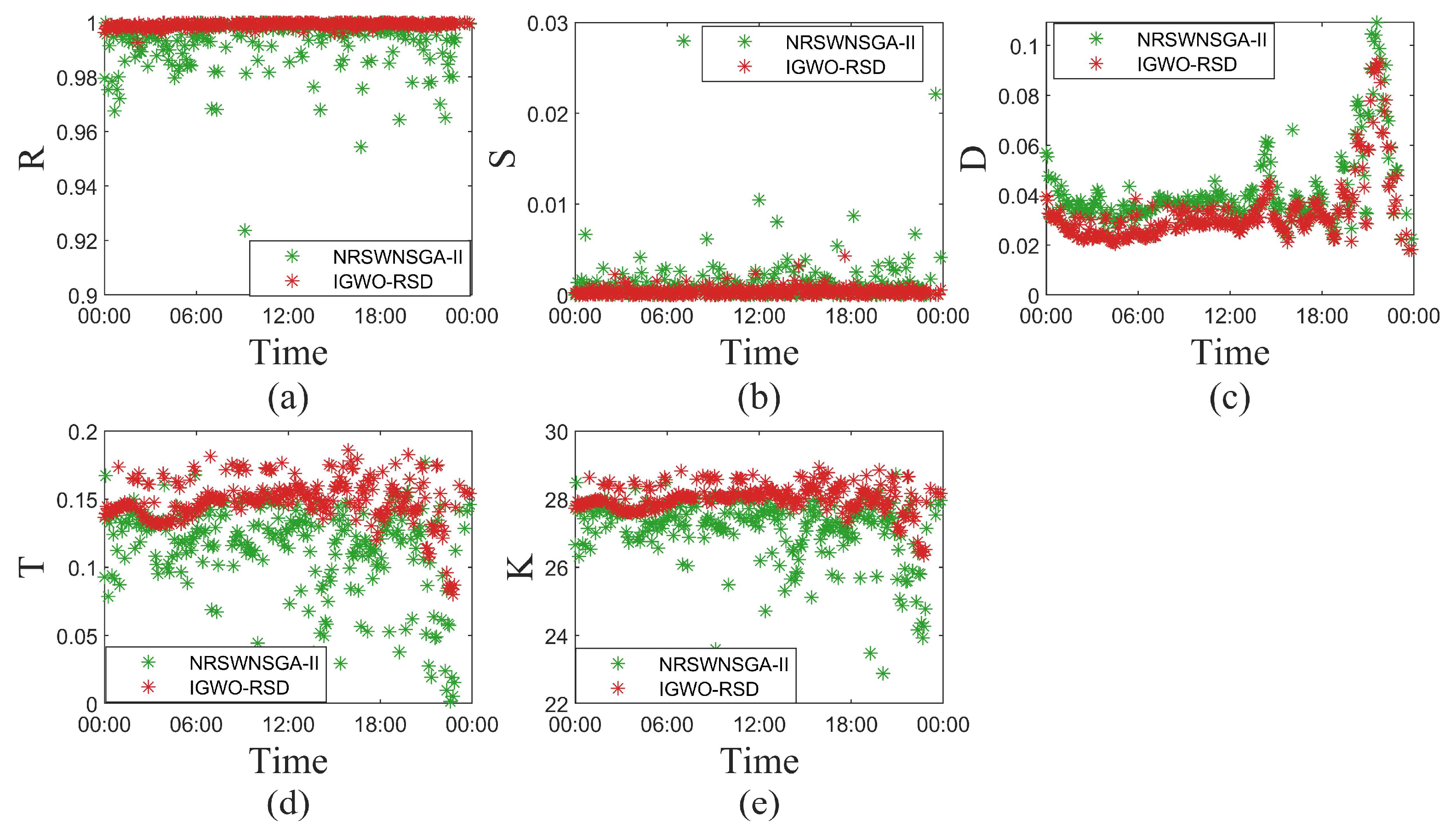
In order to demonstrate the performance of the IGWO-RSD under different signal quality conditions, samples at different time periods of the full day were employed for gluing experiments. Samples collected by the AHSRL system in Korea for the whole day of 8 May 2017 were selected to compare the performance of the two algorithms in a full-day gluing experiment. Five metrics, namely the correlation coefficient R, the regression stability coefficient S, the mean fit deviation D, the standard gain ratio deviation T and the fitting slope K were compared to provide a comprehensive analysis of the fitting results of the two algorithms. It also reflected the effectiveness of the gluing algorithm on the inversion of atmospheric optical properties.
Figure 6 shows the results of R, S, D, T and K of the two algorithms. It can be seen that the fluctuation in the gluing results by NRSWNSGA-II is much more significant than those by the IGWO-RSD. The former produces a minimum value of R = 0.9102 with a variance of 1.07 × 10⁻⁴, while the latter has a stable R, the average value of which is 0.9926 with a variance of 8.83 × 10⁻⁴. The maximum value of S obtained by NRSWNSGA-II is 0.0280, while the S of the IGWO-RSD is distributed below 0.0043. The mean value of D by NRSWNSGA-II (0.0401) is larger than that by the IGWO-RSD (0.0333). The mean and variance of the three objective functions R, S and D obtained by the IGWO-RSD are better than those of NRSWNSGA-II.
The AHSRL samples in Singapore were used in [15], in which the objective function T converges to zero. Here, we choose the AHSRL data in Korea, and the T of both algorithms does not converge to zero. It indicates that there is an error in K0 introduced by the lidar system, and the deviation from the fitting results is around 15%. The mean value of T for NRSWNSGA-II is smaller than that for the IGWO-RSD. The results of NRSWNSGA-II are better at this point, but the physical meaning of T is the deviation of the fitting slope from the prior information (K0), and in the case of inaccurate K0, T does not reflect any benefit of the gluing results. Since the physical meaning of D is the average deviation of the two-channel signals, a smaller D intuitively reflects a larger deviation in the gluing results.
The fitting slope K shows that the gluing results obtained by the IGWO-RSD are stably distributed around 28.0, with a variance of 0.09, while for those obtained by NRSWNSGA-II, the range of K spreads from 23.5936 to 28.4962 with a variance of 0.5180, and the gluing results are extremely unstable. In NRSWNSGA-II, choosing T as the objective function introduces errors in gluing if K0 itself is not accurate. Therefore, the result of D is larger and the final fitting slope K is smaller than those with IGWO-RSD. It is noticeable that the stability of all the five parameters of the IGWO-RSD is better than that of NRSWNSGA-II, which is due to the stronger global search capability of the former, as discussed in the previous section.
The comparison of the gluing results with the samples from Singapore selected from [15] is shown in Figure 7. It can be seen that the results of the IGWO-RSD in objective functions R, S and D are obviously better than NRSWNSGA-II. Unlike the gluing results from Korea, the difference in fitting slope K between the two algorithms in Singapore is not significant. The reason for this is that the standard gain ratio K0 of the AHSRL system in Singapore is more desirable than that in Korea, which has obvious errors. Generally speaking, using the mean fit deviation D instead of T excludes the possible errors caused by the prior information (introduced by using T as the objective function). Moreover, the choice of D only depends on the characteristics of the signals itself, which means that the IGWO-RSD can be used in more atmospheric lidar systems.

4. Conclusions

Gluing the multi-channel lidar signal is important but challenging in the long-range detection of atmospheric environments. In this paper, a signal gluing algorithm (IGWO-RSD) for atmospheric lidar is developed, which has advantages in terms of accuracy, stability and applicability compared with traditional algorithms, and it is also insensitive to background noise. Three measurements were taken for this purpose. First, the IGWO algorithm was adopted in lidar signal gluing for the first time, which improved the accuracy and stability in solving the optimal gluing region. Second, a fitness function consisting of three objective functions (R, S and D) is proposed, where the standard gain ratio deviation T was replaced by the mean fit deviation D to remove the effect of prior information. As a result, better accuracy and wider applicability were achieved. Objective function D also helps in signal gluing with strong background noise. Third, substituting segmented gluing for point gluing ensures the smoothness of the echo-photon profile and minimizes the distortion of the original data. It is believed that the IGWO-RSD is of great value in signal processing of the multi-channel atmospheric lidar. To maximize the performance of the algorithm, machine learning can be introduced, which will provide new solutions and ideas for lidar signal processing and analysis.

Author Contributions

Conceptualization, S.L. and D.X.; methodology, S.L. and K.Z.; software, S.L. and X.Z.; validation, S.L. and T.W.; investigation, S.L.; writing—original draft preparation, S.L.; writing—review and editing, K.Z. and T.W.; visualization, Y.S., Y.W., Y.Z. and X.L.; project administration, K.Z. and J.Y.; funding acquisition, K.Z. All authors have read and agreed to the published version of the manuscript.

Funding

This research was funded by National Natural Science Foundation of China (NSFC) grant number 62175184 and Tianjin Key Laboratory of Optoelectronic Sensor and Sensing Network Technology.

Data Availability Statement

The data presented in this study are available on request from the corresponding author.

Conflicts of Interest

The authors declare no conflict of interest.

References

  1. Singh, U.N.; Keckhut, P.; McGee, T.J.; Gross, M.R.; Hauchecorne, A.; Fishbein, E.F.; Waters, J.W.; Gille, J.C.; Roche, A.E.; Russell, J.M., III. Stratospheric Temperature Measurements by Two Collocated NDSC Lidars during UARS Validation Campaign. J. Geophys. Res. Atmos. 1996, 101, 10287–10297. [Google Scholar] [CrossRef]
  2. Yue, C. Using Rayleigh Lidar Observe and Study of the Middle Atmosphere over Beijing. Master’s Thesis, The University of Chinese Academy of Sciences, Beijing, China, 25 May 2015. [Google Scholar]
  3. Alpers, M.; Eixmann, R.; Fricke-Begemann, C.; Gerding, M.; Höffner, J. Temperature Lidar Measurements from 1 to 105 Km Altitude Using Resonance, Rayleigh, and Rotational Raman Scattering. Atmos. Chem. Phys. 2004, 4, 793–800. [Google Scholar] [CrossRef] [Green Version]
  4. Kaifler, B.; Rempel, D.; Roßi, P.; Büdenbender, C.; Kaifler, N.; Baturkin, V. A Technical Description of the Balloon Lidar Experiment (BOLIDE). Atmos. Meas. Tech. 2020, 13, 5681–5695. [Google Scholar] [CrossRef]
  5. Kaifler, B.; Kaifler, N. A Compact Rayleigh Autonomous Lidar (CORAL) for the Middle Atmosphere. Atmos. Meas. Tech. 2021, 14, 1715–1732. [Google Scholar] [CrossRef]
  6. Fu, Y.P.; Wang, Y.; Zhang, T.S.; Fan, G.Q.; Liu, W.Q.; Chang, Z.; Qiu, X.H.; Fang, L.L.; Tian, Y.Z. Signal Acquisition System with Simultaneous Analog and Photon Counting Measurement for Lidar. Chin. J. Lasers 2015, 42, 318–327. [Google Scholar]
  7. Newsom, R.K.; Turner, D.D.; Mielke, B.; Clayton, M.; Ferrare, R.; Sivaraman, C. Simultaneous Analog and Photon Counting Detection for Raman Lidar. Appl. Opt. AO 2009, 48, 3903–3914. [Google Scholar] [CrossRef] [PubMed]
  8. Zhang, Y.; Yi, F.; Kong, W.; Yi, Y. Slope Characterization in Combining Analog and Photon Count Data from Atmospheric Lidar Measurements. Appl. Opt. AO 2014, 53, 7312–7320. [Google Scholar] [CrossRef] [PubMed]
  9. D’Amico, G.; Amodeo, A.; Mattis, I.; Freudenthaler, V.; Pappalardo, G. EARLINET Calculus Chain–Technical–Part 1: Pre-Processing of Raw Lidar Data. Atmos. Meas. Tech. 2016, 9, 491–507. [Google Scholar] [CrossRef] [Green Version]
  10. Huang, L.F.; Gong, W.; Li, J.; Mao, F.Y.; Lei, L.F. Signal Splicing of Dual-Receiver Mie Scattering Lidar in Atmospheric Remote Sensing. Natl. Remote Sens. Bull. 2012, 16, 705–719. [Google Scholar]
  11. Li, J.; Gong, W.; Mao, F.Y.; Zhang, J.Y. Dual Field of View Lidar for Observing Atmospheric Aerosols over Wuhan, China. Acta Opt. Sin. 2013, 33, 9–15. [Google Scholar]
  12. Walker, M.; Venable, D.; Whiteman, D.N. Gluing for Raman Lidar Systems Using the Lamp Mapping Technique. Appl. Opt. AO 2014, 53, 8535–8543. [Google Scholar] [CrossRef] [PubMed]
  13. Gao, F.; Veberič, D.; Stanič, S.; Bergant, K.; Hua, D.-X. Performance Improvement of Long-Range Scanning Mie Lidar for the Retrieval of Atmospheric Extinction. J. Quant. Spectrosc. Radiat. Transf. 2013, 122, 72–78. [Google Scholar] [CrossRef]
  14. Gao, F.; Xu, X.; Zhu, Q.; Wang, L.; He, T.; Wang, L.; Stanič, S.; Hua, D. Evaluation and Improvement of Lidar Performance Based on Temporal and Spatial Variance Calculation. Appl. Sci. 2019, 9, 1786. [Google Scholar] [CrossRef] [Green Version]
  15. Duan, L.L.; Liu, D.; Zhang, Y.P.; Cheng, Z.T.; Luo, J.; Yang, F.Y.; Shen, Y.B.; Bai, J. Lidar Data Gluing Technology Based on Hybrid Intelligent Algorithm. Acta Opt. Sin. 2017, 37, 21–29. [Google Scholar]
  16. Mirjalili, S.; Mirjalili, S.M.; Lewis, A. Grey Wolf Optimizer. Adv. Eng. Softw. 2014, 69, 46–61. [Google Scholar] [CrossRef] [Green Version]
  17. Nadimi-Shahraki, M.H.; Taghian, S.; Mirjalili, S. An Improved Grey Wolf Optimizer for Solving Engineering Problems. Expert Syst. Appl. 2021, 166, 113917. [Google Scholar] [CrossRef]
  18. Taylor, J. Introduction to Error Analysis, the Study of Uncertainties in Physical Measurements, 2nd ed.; University Science Books: Herndon, VA, USA, 1997. [Google Scholar]
  19. An, R.M.; Suo, M.L. Application of Attributes Reduction and Weights Calculation through Neighborhood Rough Set. Comput. Eng. Appl. 2016, 52, 160–165. [Google Scholar]
  20. Hu, Q.H.; Yu, D.R.; Xie, Z.X. Numerical Attribute Reduction Based on Neighborhood Granulation and Rough Approximation. J. Softw. 2008, 19, 640–649. [Google Scholar] [CrossRef]
  21. University of Wisconsin Lidar Group. Available online: https://radiance.ssec.wisc.edu/ (accessed on 15 June 2023).
  22. Evans, R.D. The Atomic Nucleus; McGrow-Hill: New York, NY, USA, 1955; pp. 785–794. [Google Scholar]
  23. Deb, K.; Pratap, A.; Agarwal, S.; Meyarivan, T. A Fast and Elitist Multiobjective Genetic Algorithm: NSGA-II. IEEE Trans. Evol. Comput. 2002, 6, 182–197. [Google Scholar] [CrossRef] [Green Version]
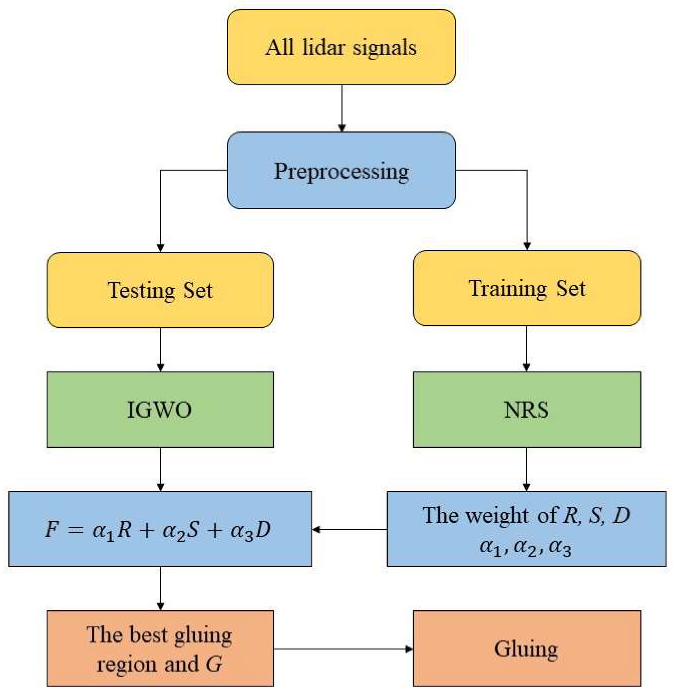
Figure 1. The flowchart of IGWO-RSD.
Remotesensing 15 03812 g001
Figure 2. Hierarchy of gray wolf.
Remotesensing 15 03812 g002
Figure 3. Comparison of midday signal gluing. (a) IGWO-RSD fitting, where the red line represents the near-field signal, the yellow line represents the far-field signal and the blue points are fitted from the far-field signal by IGWO-RSD. (b) Comparison of IGWO-RSD and NRSWNSGA-II fitting results, where the blue points are the IGWO-RSD fitting results and the purple points are the results of NRSWNSGA-II.
Remotesensing 15 03812 g003
Figure 4. Stability of midday sample gluing. (a) Stability of the fitting slope K. (b) The counts of near-channel in z0.
Remotesensing 15 03812 g004
Figure 5. Comparison of the solving abilities of the optimizers.
Remotesensing 15 03812 g005
Figure 6. Full-day gluing experiment in Korea, where the red points are results of the IGWO-RSD and the green points are the results of NRSWNSGA-II. (a) Correlation coefficient R. (b) Regression stability coefficient S. (c) Mean fit deviation D. (d) Standard gain ratio deviation T. (e) Fitting slope K.
Remotesensing 15 03812 g006
Figure 7. Full-day gluing experiment in Singapore, where the red points are the results of the IGWO-RSD, and the green points are the results of NRSWNSGA-II. (a) Correlation coefficient R. (b) Regression stability coefficient S. (c) Mean fit deviation D. (d) Standard gain ratio deviation T. (e) Fitting slope K.
Remotesensing 15 03812 g007
Table 1. Criterion of objective function hierarchical scoring.
Property PointR/%S/%D/%
0[99, 100][0, 0.1][0, 0.05]
1[98, 99)(0.1, 0.2](0.05, 0.1]
2[96, 98)(0.2, 0.4](0.1, 0.2]
3[92, 96)(0.4, 0.6](0.2, 0.3]
4ElseElseElse
Table 2. Operating parameters of the algorithms.
ParameterValueParameterValue
Number of wolves100Number of iterations70
Weight of R0.4102Lower limit of R0.9
Weight of S0.2233Time resolution of samples60 min
Weight of D0.3665Vertical resolution of samples7.5 m
Disclaimer/Publisher’s Note: The statements, opinions and data contained in all publications are solely those of the individual author(s) and contributor(s) and not of MDPI and/or the editor(s). MDPI and/or the editor(s) disclaim responsibility for any injury to people or property resulting from any ideas, methods, instructions or products referred to in the content.