
MFSFNet: Multi-Scale Feature Subtraction Fusion Network for Remote Sensing Image Change Detection

Abstract
:
1. Introduction
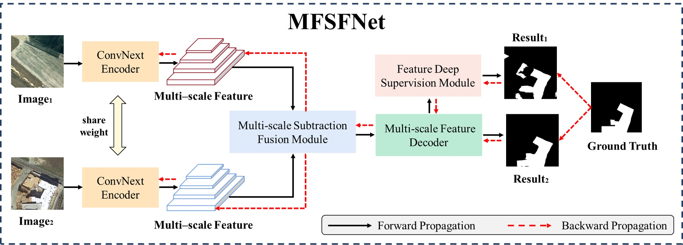
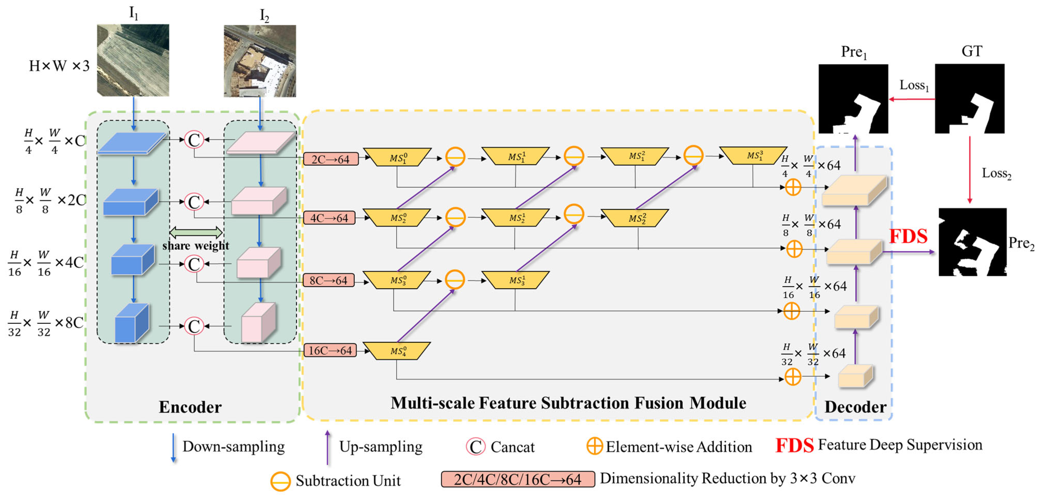
- We propose the MFSFNet for high-resolution remote sensing image change detection. This network enhances change features and reduces redundant pseudo-change features through a multi-scale subtraction fusion strategy.
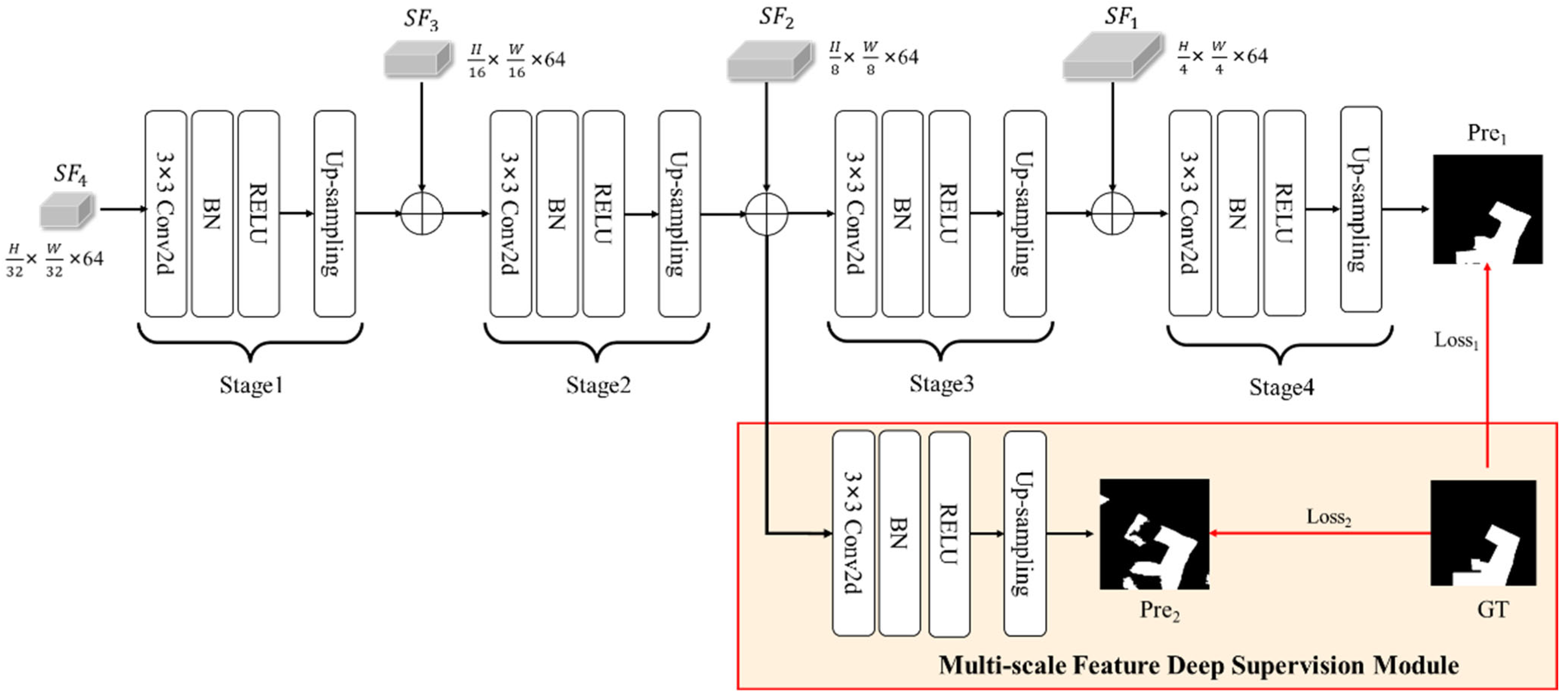
- We utilize a lightweight feature extraction network and introduce a novel deep supervision strategy in the change decoder, which enhances the training performance of the network.
2. Related Works
2.1. Encoder in Change Detection Task
2.2. Multi-Scale Feature Fusion in Change Detection Task
3. Methods
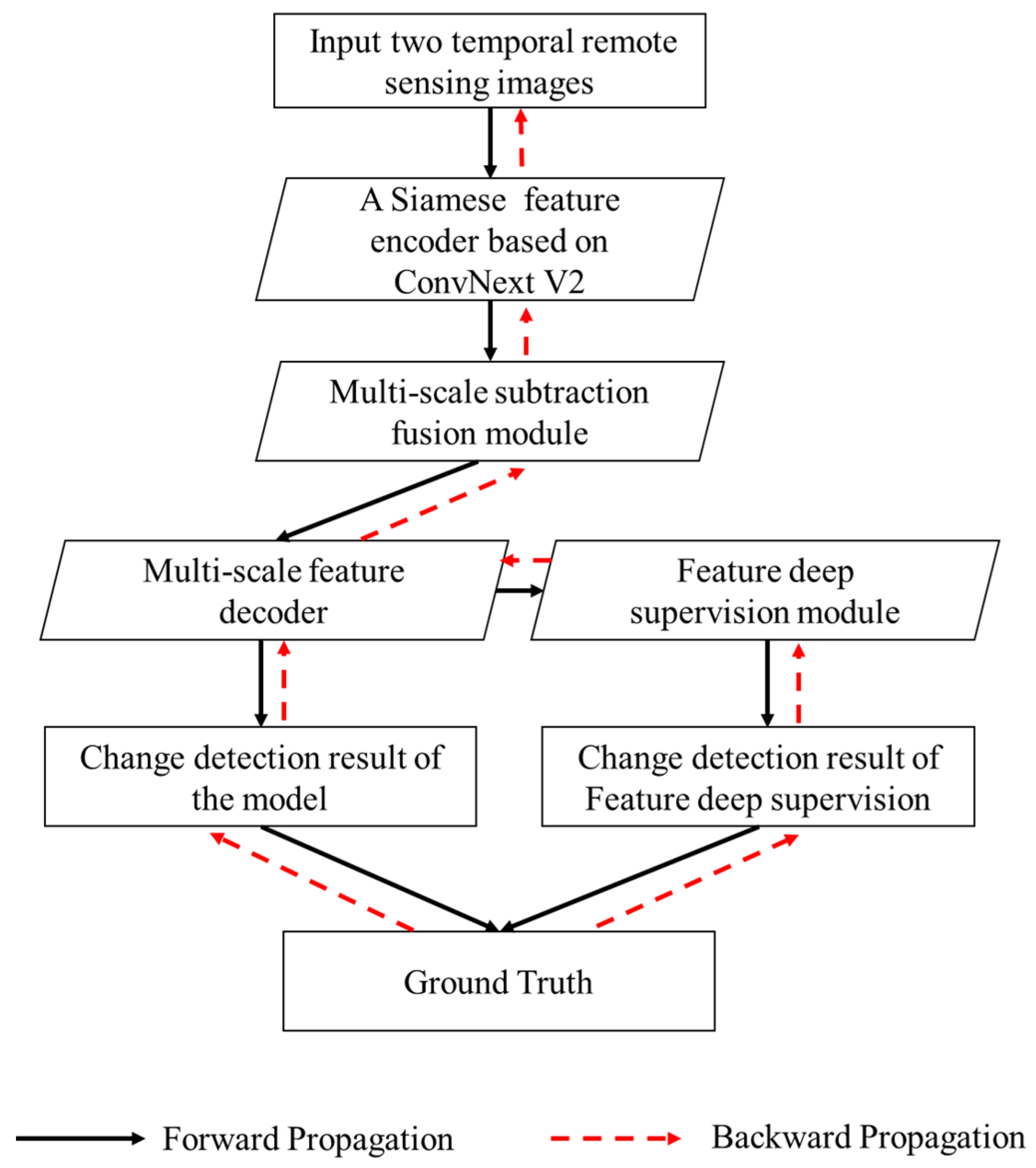
3.1. Flowchart and Overall Architecture of MFSFNet
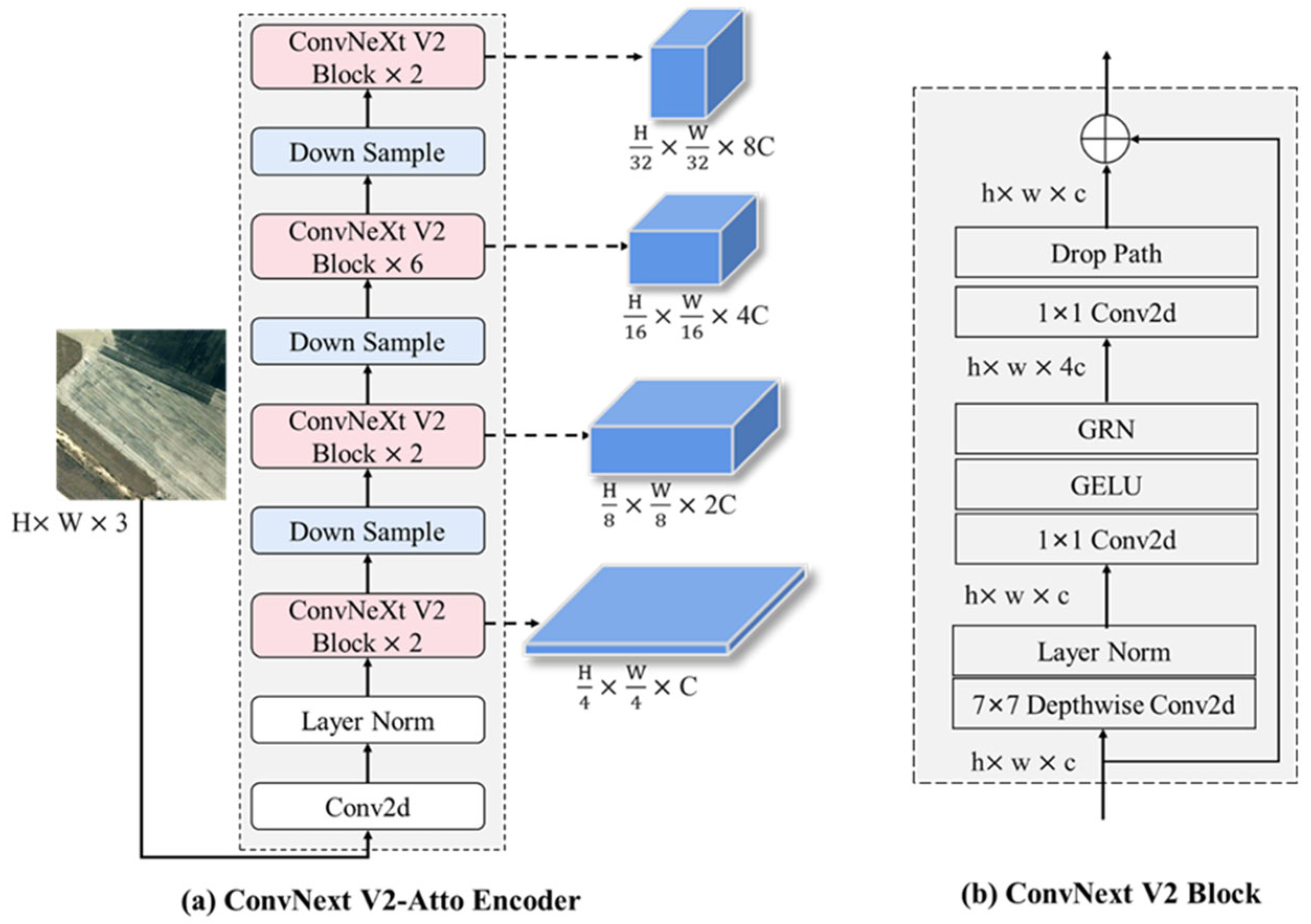
3.2. The Siamese Feature Encoder
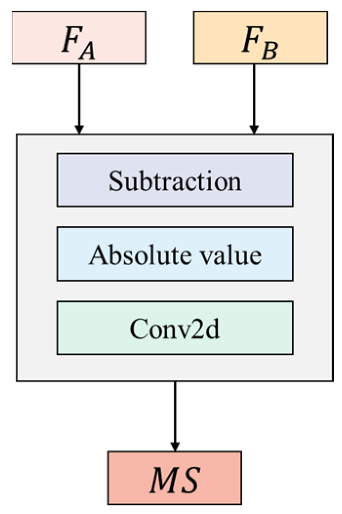
3.3. Multi-Scale Feature Subtraction Fusion (MSSF) Module
3.4. Decoder and Feature Deep Supervision Module
3.5. Loss Function of MFSFNet
4. Experiments
4.1. Datasets
- (1)
- LEVIR-CD
- (2)
- CDD
4.2. Evaluation Metrics
4.3. Implementation Details
4.4. Comparative Methods
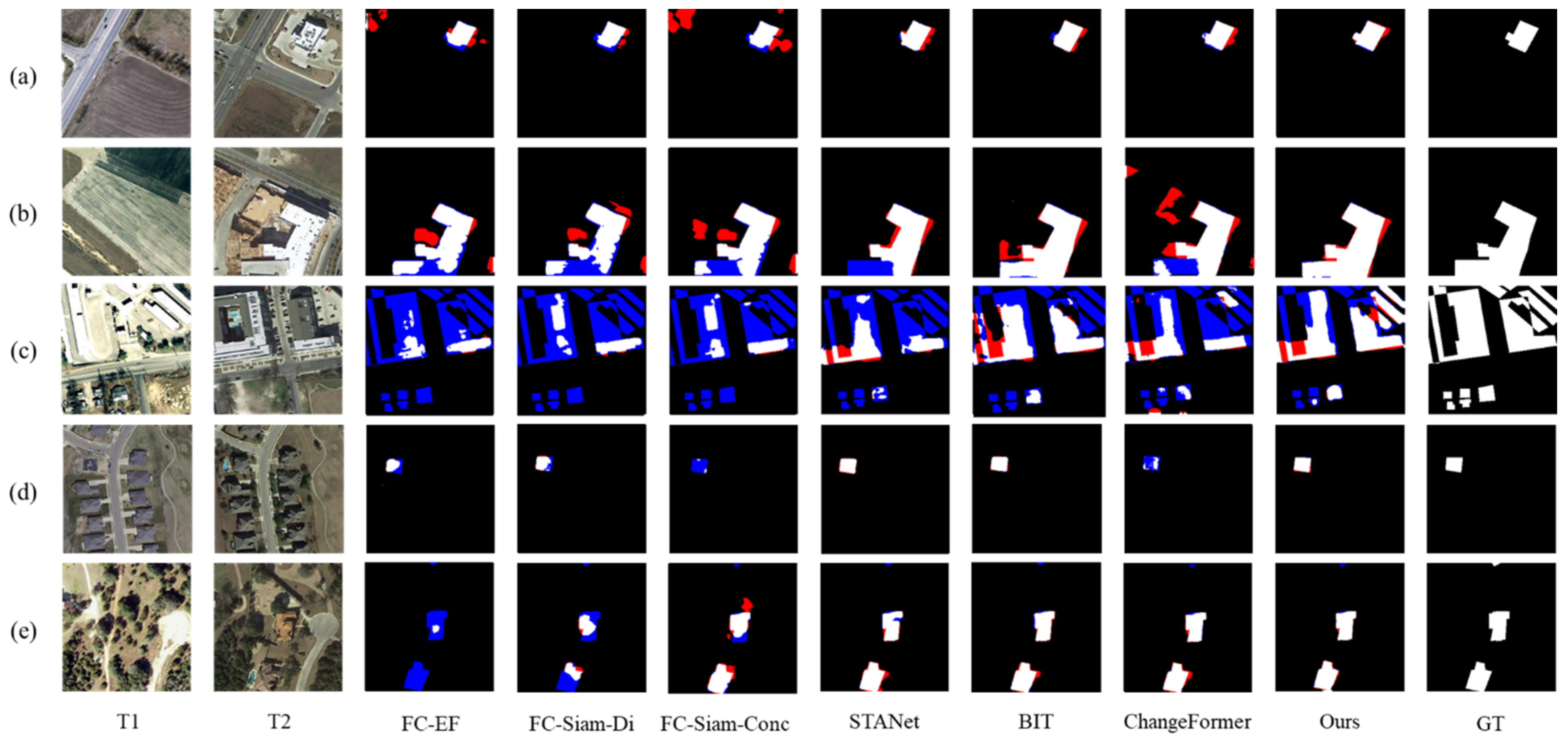
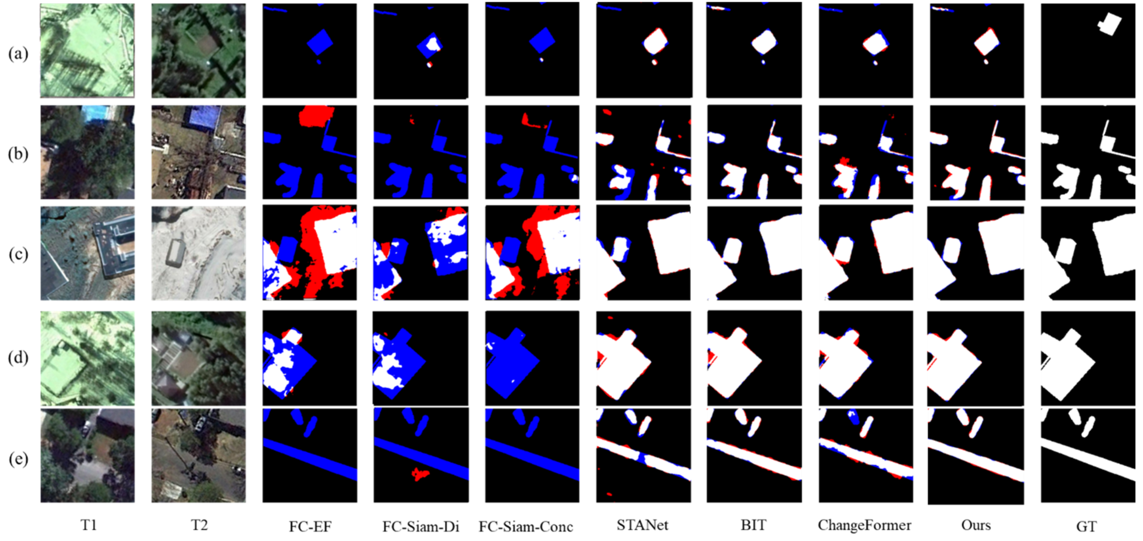
- FC-EF [37], FC-Siam-conc [37], and FC-Siam-diff [37] were the first methods to introduce Siamese networks into change detection. EF refers to a fusion technique in which the dual-temporal images are combined or merged at the input stage. Siam-conc represents the concatenation fusion model based on Siamese networks, which combines the dual-temporal features. Siam-diff represents the difference fusion model based on Siamese networks.
- STANet [53] incorporates a self-attention feature fusion module, enabling the model to capture the spatiotemporal dependencies present in various sub-regions of the input images. The self-attention mechanism allows the network to concentrate on important regions and relationships within the images, enhancing its ability to detect changes effectively.
- BiT [35] leverages the Transformer architecture as a change feature fusion network, integrating it with a convolutional neural network (CNN) backbone. This combination enables BiT to capture and model the global semantic information from dual-temporal features. By incorporating Transformers, which excel at capturing long-range dependencies and contextual information, BiT enhances the representation learning process and performance. The CNN backbone complements the Transformer by extracting spatial features from the input images. Together, they form a powerful framework for effectively detecting changes in remote-sensing data.
- ChangeFormer [64] is a change detection method that utilizes a pure Transformer architecture. Unlike traditional methods that combine CNNs and Transformers, ChangeFormer solely relies on Transformers for the entire change detection process. By leveraging the self-attention mechanism, ChangeFormer efficiently captures multi-scale long-range details. The Transformer architecture allows for the modeling of global dependencies and contextual information across the input images, enhancing the overall performance of change detection tasks.
4.5. Results Evaluation
4.5.1. Experimental Results on LEVIR-CD
4.5.2. Experimental Results on CDD
5. Discussion
5.1. Ablation Experiments
5.1.1. The Ablation of MFSF and FDS
5.1.2. The Effectiveness of MFSF
5.2. Parameter Analysis
6. Conclusions
Author Contributions
Funding
Data Availability Statement
Conflicts of Interest
References
- Singh, A. Review article digital change detection techniques using remotely-sensed data. Int. J. Remote Sens. 1989, 10, 989–1003. [Google Scholar] [CrossRef] [Green Version]
- Zhong, Q.; Ma, J.; Zhao, B.; Wang, X.; Zong, J.; Xiao, X. Assessing spatial-temporal dynamics of urban expansion, vegetation greenness and photosynthesis in megacity Shanghai, China during 2000–2016. Remote Sens. Environ. 2019, 233, 111374. [Google Scholar] [CrossRef]
- De Moel, H.; Jongman, B.; Kreibich, H.; Merz, B.; Penning-Rowsell, E.; Ward, P.J. Flood risk assessments at different spatial scales. Mitig. Adapt. Strat. Glob. Chang. 2015, 20, 865–890. [Google Scholar] [CrossRef] [Green Version]
- Demir, B.; Bovolo, F.; Bruzzone, L. Updating Land-Cover Maps by Classification of Image Time Series: A Novel Change-Detection-Driven Transfer Learning Approach. IEEE Trans. Geosci. Remote Sens. 2013, 51, 300–312. [Google Scholar] [CrossRef]
- Mondini, A.C.; Guzzetti, F.; Reichenbach, P.; Rossi, M.; Cardinali, M.; Ardizzone, F. Semi-automatic recognition and mapping of rainfall induced shallow landslides using optical satellite images. Remote Sens. Environ. 2011, 115, 1743–1757. [Google Scholar] [CrossRef]
- Du, P.; Wang, X.; Chen, D.; Liu, S.; Lin, C.; Meng, Y. An improved change detection approach using tri-temporal logic-verified change vector analysis. ISPRS J. Photogramm. Remote Sens. 2020, 161, 278–293. [Google Scholar] [CrossRef]
- Lambin, E.F.; Strahlers, A.H. Change-vector analysis in multitemporal space: A tool to detect and categorize land-cover change processes using high temporal-resolution satellite data. Remote Sens. Environ. 1994, 48, 231–244. [Google Scholar] [CrossRef]
- Kesikoglu, M.H.; Atasever, .H.; Özkan, C. Unsupervised change detection in satellite images using fuzzy c-means clustering and principal component analysis. ISPRS Int. Arch. Photogramm. Remote Sens. Spat. Inf. Sci. 2013, XL7, 129–132. [Google Scholar] [CrossRef] [Green Version]
- Celik, T. Unsupervised Change Detection in Satellite Images Using Principal Component Analysis and k-Means Clustering. IEEE Geosci. Remote Sens. Lett. 2009, 6, 772–776. [Google Scholar] [CrossRef]
- Zhong, J.; Wang, R. Multi-temporal remote sensing change detection based on independent component analysis. Int. J. Remote Sens. 2006, 27, 2055–2061. [Google Scholar] [CrossRef]
- Gong, M.; Yang, Y.-H. Quadtree-based genetic algorithm and its applications to computer vision. Pattern Recognit. 2004, 37, 1723–1733. [Google Scholar] [CrossRef]
- Baraldi, A.; Boschetti, L. Operational Automatic Remote Sensing Image Understanding Systems: Beyond Geographic Object-Based and Object-Oriented Image Analysis (GEOBIA/GEOOIA). Part 1: Introduction. Remote Sens. 2012, 4, 2694–2735. [Google Scholar] [CrossRef] [Green Version]
- Roy, S.K.; Krishna, G.; Dubey, S.R.; Chaudhuri, B.B. HybridSN: Exploring 3-D–2-D CNN Feature Hierarchy for Hyperspectral Image Classification. IEEE Geosci. Remote Sens. Lett. 2020, 17, 277–281. [Google Scholar] [CrossRef] [Green Version]
- Mou, L.; Ghamisi, P.; Zhu, X.X. Deep Recurrent Neural Networks for Hyperspectral Image Classification. IEEE Trans. Geosci. Remote Sens. 2017, 55, 3639–3655. [Google Scholar] [CrossRef] [Green Version]
- Kampffmeyer, M.; Salberg, A.-B.; Jenssen, R. Semantic Segmentation of Small Objects and Modeling of Uncertainty in Urban Remote Sensing Images Using Deep Convolutional Neural Networks. In Proceedings of the 2016 IEEE Conference on Computer Vision and Pattern Recognition Workshops (CVPRW), Las Vegas, NV, USA, 26 June–1 July 2016; pp. 1–9. [Google Scholar] [CrossRef]
- Kemker, R.; Salvaggio, C.; Kanan, C. Algorithms for semantic segmentation of multispectral remote sensing imagery using deep learning. ISPRS J. Photogramm. Remote Sens. 2018, 145, 60–77. [Google Scholar] [CrossRef] [Green Version]
- Zhao, H.; Shi, J.; Qi, X.; Wang, X.; Jia, J. Pyramid scene parsing network. In Proceedings of the 2017 IEEE Conference on Computer Vision and Pattern Recognition, Honolulu, HI, USA, 21–26 July 2017; pp. 2881–2890. [Google Scholar]
- Shivappriya, S.N.; Priyadarsini, M.J.P.; Stateczny, A.; Puttamadappa, C.; Parameshachari, B.D. Cascade Object Detection and Remote Sensing Object Detection Method Based on Trainable Activation Function. Remote Sens. 2021, 13, 200. [Google Scholar] [CrossRef]
- Avola, D.; Cinque, L.; Diko, A.; Fagioli, A.; Foresti, G.L.; Mecca, A.; Pannone, D.; Piciarelli, C. MS-Faster R-CNN: Multi-Stream Backbone for Improved Faster R-CNN Object Detection and Aerial Tracking from UAV Images. Remote Sens. 2021, 13, 1670. [Google Scholar] [CrossRef]
- Yang, M.; Jiao, L.; Liu, F.; Hou, B.; Yang, S. Transferred Deep Learning-Based Change Detection in Remote Sensing Images. IEEE Trans. Geosci. Remote Sens. 2019, 57, 6960–6973. [Google Scholar] [CrossRef]
- Li, X.; He, M.; Li, H.; Shen, H. A Combined Loss-Based Multiscale Fully Convolutional Network for High-Resolution Remote Sensing Image Change Detection. IEEE Geosci. Remote Sens. Lett. 2022, 19, 1–5. [Google Scholar] [CrossRef]
- Zhang, H.; Gong, M.; Zhang, P.; Su, L.; Shi, J. Feature-Level Change Detection Using Deep Representation and Feature Change Analysis for Multispectral Imagery. IEEE Geosci. Remote Sens. Lett. 2016, 13, 1666–1670. [Google Scholar] [CrossRef]
- Lv, Z.; Wang, F.; Cui, G.; Benediktsson, J.A.; Lei, T.; Sun, W. Spatial–Spectral Attention Network Guided with Change Magnitude Image for Land Cover Change Detection Using Remote Sensing Images. IEEE Trans. Geosci. Remote Sens. 2022, 60, 1–12. [Google Scholar] [CrossRef]
- Chen, T.; Lu, Z.; Yang, Y.; Zhang, Y.; Du, B.; Plaza, A.J. A Siamese Network Based U-Net for Change Detection in High Resolution Remote Sensing Images. IEEE J. Sel. Top. Appl. Earth Obs. Remote Sens. 2022, 15, 2357–2369. [Google Scholar] [CrossRef]
- Peng, D.; Zhang, Y.; Guan, H. End-to-End Change Detection for High Resolution Satellite Images Using Improved UNet++. Remote Sens. 2019, 11, 1382. [Google Scholar] [CrossRef] [Green Version]
- Du, P.; Liu, S.; Xia, J.; Zhao, Y. Information Fusion Techniques for Change Detection from Multi-Temporal Remote Sensing Images. Inf. Fusion 2013, 14, 19–27. [Google Scholar] [CrossRef]
- Alimjan, G.; Jiaermuhamaiti, Y.; Jumahong, H.; Zhu, S.; Nurmamat, P. An Image Change Detection Algorithm Based on Multi-Feature Self-Attention Fusion Mechanism UNet Network. Int. J. Pattern Recogn. Artif. Intell. 2021, 35, 2159049. [Google Scholar] [CrossRef]
- Jiang, Y.; Hu, L.; Zhang, Y.; Yang, X. WRICNet: A Weighted Rich-Scale Inception Coder Network for Multi-Resolution Remote Sensing Image Change Detection. IEEE Trans. Geosci. Remote Sens. 2022, 60, 1–13. [Google Scholar] [CrossRef]
- Fang, S.; Li, K.; Shao, J.; Li, Z. SNUNet-CD: A Densely Connected Siamese Network for Change Detection of VHR Images. IEEE Geosci. Remote Sens. Lett. 2022, 19, 1–5. [Google Scholar] [CrossRef]
- Shi, Q.; Liu, M.; Li, S.; Liu, X.; Wang, F.; Zhang, L. A Deeply Supervised Attention Metric-Based Network and an Open Aerial Image Dataset for Remote Sensing Change Detection. IEEE Trans. Geosci. Remote Sens. 2022, 60, 1–16. [Google Scholar] [CrossRef]
- Chen, J.; Yuan, Z.; Peng, J.; Chen, L.; Huang, H.; Zhu, J.; Liu, Y.; Li, H. DASNet: Dual Attentive Fully Convolutional Siamese Networks for Change Detection in High-Resolution Satellite Images. IEEE J. Sel. Top. Appl. Earth Obs. Remote Sens. 2021, 14, 1194–1206. [Google Scholar] [CrossRef]
- Ding, Q.; Shao, Z.; Huang, X.; Altan, O. DSA-Net: A novel deeply supervised attention-guided network for building change detection in high-resolution remote sensing images. Int. J. Appl. Earth Obs. Geoinf. 2021, 105, 102591. [Google Scholar] [CrossRef]
- Yang, L.; Chen, Y.; Song, S.; Li, F.; Huang, G. Deep Siamese Networks Based Change Detection with Remote Sensing Images. Remote Sens. 2021, 13, 3394. [Google Scholar] [CrossRef]
- Chen, H.; Wu, C.; Du, B. Towards Deep and Efficient: A Deep Siamese Self-Attention Fully Efficient Convolutional Network for Change Detection in VHR Images. arXiv 2021, arXiv:2108.08157. [Google Scholar]
- Chen, H.; Qi, Z.; Shi, Z. Remote Sensing Image Change Detection with Transformers. IEEE Trans. Geosci. Remote Sens. 2022, 60, 1–14. [Google Scholar] [CrossRef]
- Zhang, C.; Yue, P.; Tapete, D.; Jiang, L.; Shangguan, B.; Huang, L.; Liu, G. A deeply supervised image fusion network for change detection in high resolution bi-temporal remote sensing images. ISPRS J. Photogramm. Remote Sens. 2020, 166, 183–200. [Google Scholar] [CrossRef]
- Caye Daudt, R.; Le Saux, B.; Boulch, A. Fully Convolutional Siamese Networks for Change Detection. In Proceedings of the 2018 25th IEEE International Conference on Image Processing (ICIP), Athens, Greece, 7–10 October 2018; pp. 4063–4067. [Google Scholar]
- Zhao, W.; Mou, L.; Chen, J.; Bo, Y.; Emery, W.J. Incorporating Metric Learning and Adversarial Network for Seasonal Invariant Change Detection. IEEE Trans. Geosci. Remote Sens. 2020, 58, 2720–2731. [Google Scholar] [CrossRef]
- Hou, B.; Liu, Q.; Wang, H.; Wang, Y. From W-Net to CDGAN: Bitemporal Change Detection via Deep Learning Techniques. IEEE Trans. Geosci. Remote Sens. 2020, 58, 1790–1802. [Google Scholar] [CrossRef] [Green Version]
- Lebedev, M.A.; Vizilter, Y.V.; Vygolov, O.V.; Knyaz, V.A.; Rubis, A.Y. Change detection in remote sensing images using conditional adversarial networks. ISPRS Int. Arch. Photogramm. Remote Sens. Spat. Inf. Sci. 2018, 422, 565–571. [Google Scholar] [CrossRef] [Green Version]
- Khusni, U.; Dewangkoro, H.I.; Arymurthy, A.M. Urban Area Change Detection with Combining CNN and RNN from Sentinel-2 Multispectral Remote Sensing Data. In Proceedings of the 2020 3rd International Conference on Computer and Informatics Engineering (IC2IE), Yogyakarta, Indonesia, 15–16 September 2020; pp. 171–175. [Google Scholar]
- Papadomanolaki, M.; Verma, S.; Vakalopoulou, M.; Gupta, S.; Karantzalos, K. Detecting Urban Changes with Recurrent Neural Networks from Multitemporal Sentinel-2 Data. In Proceedings of the IGARSS 2019—2019 IEEE International Geoscience and Remote Sensing Symposium, Yokohama, Japan, 28 July–2 August 2019; pp. 214–217. [Google Scholar]
- Mohammadian, A.; Ghaderi, F. SiamixFormer: A fully-transformer Siamese network with temporal Fusion for accurate building detection and change detection in bi-temporal remote sensing images. Int. J. Remote Sens. 2023, 44, 3660–3678. [Google Scholar] [CrossRef]
- Shafique, A.; Seydi, S.T.; Alipour-Fard, T.; Cao, G.; Yang, D. SSViT-HCD: A Spatial Spectral Convolutional Vision Transformer for Hyperspectral Change Detection. IEEE J. Sel. Top. Appl. Earth Obs. Remote Sens. 2023, 16, 6487–6504. [Google Scholar] [CrossRef]
- Marsocci, V.; Coletta, V.; Ravanelli, R.; Scardapane, S.; Crespi, M. Inferring 3D change detection from bitemporal optical images. ISPRS J. Photogramm. Remote Sens. 2023, 196, 325–339. [Google Scholar] [CrossRef]
- Peng, X.; Zhong, R.; Li, Z.; Li, Q. Optical Remote Sensing Image Change Detection Based on Attention Mechanism and Image Difference. IEEE Trans. Geosci. Remote Sens. 2021, 59, 7296–7307. [Google Scholar] [CrossRef]
- Wang, D.; Chen, X.; Jiang, M.; Du, S.; Xu, B.; Wang, J. ADS-Net:An Attention-Based deeply supervised network for remote sensing image change detection. Int. J. Appl. Earth Obs. Geoinf. 2021, 101, 102348. [Google Scholar] [CrossRef]
- Yu, X.; Fan, J.; Chen, J.; Zhang, P.; Zhou, Y.; Han, L. NestNet: A multiscale convolutional neural network for remote sensing image change detection. Int. J. Remote Sens. 2021, 42, 4898–4921. [Google Scholar] [CrossRef]
- Yu, X.; Fan, J.; Zhang, P.; Han, L.; Zhang, D.; Sun, G. Multi-Scale Convolutional Neural Network for Remote Sensing Image Change Detection. In Proceedings of the Geoinformatics in Sustainable Ecosystem and Society; Xie, Y., Li, Y., Yang, J., Xu, J., Deng, Y., Eds.; Springer: Singapore, 2020; pp. 234–242. [Google Scholar]
- Zhou, Z.; Rahman Siddiquee, M.M.; Tajbakhsh, N.; Liang, J. UNet++: A Nested U-Net Architecture for Medical Image Segmentation. In Proceedings of the Deep Learning in Medical Image Analysis and Multimodal Learning for Clinical Decision Support; Stoyanov, D., Taylor, Z., Carneiro, G., Syeda-Mahmood, T., Martel, A., Maier-Hein, L., Tavares, J.M.R.S., Bradley, A., Papa, J.P., Belagiannis, V., et al., Eds.; Springer International Publishing: Cham, Switzerland, 2018; pp. 3–11. [Google Scholar]
- Ronneberger, O.; Fischer, P.; Brox, T. U-Net: Convolutional Networks for Biomedical Image Segmentation. In Proceedings of the Medical Image Computing and Computer-Assisted Intervention—MICCAI 2015; Navab, N., Hornegger, J., Wells, W.M., Frangi, A.F., Eds.; Springer International Publishing: Cham, Switzerland, 2015; pp. 234–241. [Google Scholar]
- Zhan, Y.; Fu, K.; Yan, M.; Sun, X.; Wang, H.; Qiu, X. Change Detection Based on Deep Siamese Convolutional Network for Optical Aerial Images. IEEE Geosci. Remote Sens. Lett. 2017, 14, 1845–1849. [Google Scholar] [CrossRef]
- Chen, H.; Shi, Z. A Spatial-Temporal Attention-Based Method and a New Dataset for Remote Sensing Image Change Detection. Remote Sens. 2020, 12, 1662. [Google Scholar] [CrossRef]
- He, K.; Zhang, X.; Ren, S.; Sun, J. Deep residual learning for image recognition. In Proceedings of the IEEE Computer Society Conference on Computer Vision and Pattern Recognition (CVPR), Las Vegas, NV, USA, 27–30 June 2016; pp. 770–778. [Google Scholar] [CrossRef] [Green Version]
- Zhang, M.; Xu, G.; Chen, K.; Yan, M.; Sun, X. Triplet-Based Semantic Relation Learning for Aerial Remote Sensing Image Change Detection. IEEE Geosci. Remote Sens. Lett. 2019, 16, 266–270. [Google Scholar] [CrossRef]
- Meshkini, K.; Bovolo, F.; Bruzzone, L. A 3D CNN approach for change detection in HR satellite image time series based on a pretrained 2D CNN. ISPRS—Int. Arch. Photogramm. Remote Sens. Spat. Inf. Sci. 2022, 43, 143–150. [Google Scholar] [CrossRef]
- Liu, Z.; Mao, H.; Wu, C.-Y.; Feichtenhofer, C.; Darrell, T.; Xie, S. A ConvNet for the 2020s. In Proceedings of the 2022 IEEE/CVF Conference on Computer Vision and Pattern Recognition (CVPR), New Orleans, LA, USA, 18–24 June 2022; pp. 11966–11976. [Google Scholar] [CrossRef]
- Woo, S.; Debnath, S.; Hu, R.; Chen, X.; Liu, Z.; Kweon, I.S.; Xie, S. ConvNeXt V2: Co-Designing and Scaling ConvNets with Masked Autoencoders. arXiv 2023, arXiv:2301.00808. [Google Scholar]
- He, K.; Chen, X.; Xie, S.; Li, Y.; Dollar, P.; Girshick, R. Masked Autoencoders Are Scalable Vision Learners. In Proceedings of the IEEE/CVF Conference on Computer Vision and Pattern Recognition (CVPR), New Orleans, LA, USA, 18–24 June 2022; pp. 16000–16009. [Google Scholar] [CrossRef]
- Chollet, F. Xception: Deep Learning with Depthwise Separable Convolutions. In Proceedings of the 2017 IEEE Conference on Computer Vision and Pattern Recognition (CVPR), Honolulu, HI, USA, 21–26 July 2017; pp. 1800–1807. [Google Scholar]
- Ba, J.L.; Kiros, J.R.; Hinton, G.E. Layer Normalization. arXiv 2016, arXiv:1607.06450, 2016. [Google Scholar]
- Hendrycks, D.; Gimpel, K. Gaussian Error Linear Units (GELUs). arXiv 2020, arXiv:1606.08415. [Google Scholar]
- Milletari, F.; Navab, N.; Ahmadi, S.-A. V-net: Fully convolutional neural networks for volumetric medical image segmentation. arXiv 2016, arXiv:1606.04797. [Google Scholar]
- Bandara, W.G.C.; Patel, V.M. A Transformer-Based Siamese Network for Change Detection. In Proceedings of the IGARSS 2022–2022 IEEE International Geoscience and Remote Sensing Symposium, Kuala Lumpur, Malaysia, 17–22 July 2022; pp. 207–210. [Google Scholar]


| Method | Encoder Architecture | Feature Fusion Strategy | Proposed Year |
|---|---|---|---|
| Siamese convolutional networks [52] | Twin networks with shared weights. | N/A | 2017 |
| FC-EF, FC-Siam-conc, FC-Siam-diff [37] | Fully connected layer skip connecting. | Concatenation | 2018 |
| Unet++_MSOF [25] | Multi-scale feature for combining low-level and high-level information. | Addition | 2019 |
| Dilated convolutions [55] | Twin networks with shared weights and dilated convolutions used instead of traditional convolutions. | Concatenation | 2019 |
| STANet [53] | Twin networks with shared weights and ResNet used as the backbone. | Addition | 2020 |
| PSPNet-CONC [49] | Introduces PSP module for multi-scale feature extraction and contextual information capture. | Addition | 2020 |
| DASNet [31] | Twin networks with shared weights and ResNet used as the backbone. | Addition | 2021 |
| NestNet [48] | Multi-scale feature for combining low-level and high-level information. | Addition | 2021 |
| ADS-Net [47] | Multi-scale feature for combining low-level and high-level information. | Addition | 2021 |
| SNUNet-CD [29] | Employs dense connections between features at layers. | Addition | 2022 |
| 3D CNN [56] | A 3D CNN based on a pretrained 2D CNN | Concatenation | 2022 |
| Precision (%) | Recall (%) | F1 (%) | IoU (%) | |
|---|---|---|---|---|
| FC-EF | 80.24 | 70.31 | 74.95 | 59.93 |
| FC-Siam-Di | 85.32 | 74.82 | 79.72 | 66.28 |
| FC-Siam-conc | 83.82 | 81.98 | 82.89 | 70.77 |
| STANet | 91.90 | 85.00 | 88.10 | 79.12 |
| BIT | 89.24 | 89.37 | 89.31 | 80.68 |
| ChangeFormer | 92.05 | 88.80 | 90.40 | 82.84 |
| Ours | 92.16 | 90.17 | 91.15 | 83.75 |
| Precision (%) | Recall (%) | F1 (%) | IoU (%) | |
|---|---|---|---|---|
| FC-EF | 66.73 | 54.08 | 59.74 | 42.59 |
| FC-Siam-Di | 81.51 | 51.68 | 63.25 | 46.25 |
| FC-Siam-conc | 72.60 | 46.58 | 56.75 | 39.62 |
| STANet | 92.28 | 85.44 | 88.61 | 80.12 |
| BIT | 96.02 | 93.26 | 94.61 | 89.78 |
| ChangeFormer | 94.50 | 93.52 | 94.23 | 89.09 |
| Ours | 95.59 | 95.70 | 95.64 | 91.65 |
| Encoder | MFSF Module | The Stage of Deep Supervision for FDS Module | F1 (%) | ||||
|---|---|---|---|---|---|---|---|
| Atto | Tiny | 1 | 2 | 3 | 4 | ||
| √ | √ | 88.52 | |||||
| √ | √ | √ | 89.25 | ||||
| √ | √ | √ | √ | 89.51 | |||
| √ | √ | √ | √ | √ | 89.20 | ||
| √ | √ | √ | √ | √ | √ | 89.31 | |
| √ | √ | √ | √ | 91.15 | |||
| Fusion Strategy | Precision (%) | Recall (%) | F1 (%) | IoU (%) |
|---|---|---|---|---|
| Product | 90.65 | 87.66 | 89.13 | 80.39 |
| Concatenate | 90.30 | 88.33 | 89.31 | 80.68 |
| Maximum | 90.59 | 87.49 | 89.02 | 80.21 |
| Average | 90.42 | 87.62 | 89.00 | 80.18 |
| Addition | 90.88 | 87.17 | 88.98 | 80.15 |
| Ours | 91.26 | 88.17 | 89.51 | 81.30 |
| Activation Function | Precision (%) | Recall (%) | F1 (%) | IoU (%) |
|---|---|---|---|---|
| ReLU | 90.80 | 88.12 | 89.40 | 81.16 |
| Absolute Value | 91.26 | 88.17 | 89.51 | 81.30 |
Disclaimer/Publisher’s Note: The statements, opinions and data contained in all publications are solely those of the individual author(s) and contributor(s) and not of MDPI and/or the editor(s). MDPI and/or the editor(s) disclaim responsibility for any injury to people or property resulting from any ideas, methods, instructions or products referred to in the content. |
© 2023 by the authors. Licensee MDPI, Basel, Switzerland. This article is an open access article distributed under the terms and conditions of the Creative Commons Attribution (CC BY) license (https://creativecommons.org/licenses/by/4.0/).
Share and Cite
Huang, Z.; You, H. MFSFNet: Multi-Scale Feature Subtraction Fusion Network for Remote Sensing Image Change Detection. Remote Sens. 2023, 15, 3740. https://doi.org/10.3390/rs15153740
Huang Z, You H. MFSFNet: Multi-Scale Feature Subtraction Fusion Network for Remote Sensing Image Change Detection. Remote Sensing. 2023; 15(15):3740. https://doi.org/10.3390/rs15153740
Chicago/Turabian StyleHuang, Zhiqi, and Hongjian You. 2023. "MFSFNet: Multi-Scale Feature Subtraction Fusion Network for Remote Sensing Image Change Detection" Remote Sensing 15, no. 15: 3740. https://doi.org/10.3390/rs15153740
APA StyleHuang, Z., & You, H. (2023). MFSFNet: Multi-Scale Feature Subtraction Fusion Network for Remote Sensing Image Change Detection. Remote Sensing, 15(15), 3740. https://doi.org/10.3390/rs15153740