Active Navigation System for a Rubber-Tapping Robot Based on Trunk Detection

Abstract

To address the practical navigation issues of rubber-tapping robots, this paper proposes an active navigation system guided by trunk detection for a rubber-tapping robot. A tightly coupled sliding-window-based factor graph method is proposed for pose tracking, which introduces normal distribution transform (NDT) measurement factors, inertial measurement unit (IMU) pre-integration factors, and prior factors generated by sliding window marginalization. To actively pursue goals in navigation, a distance-adaptive Euclidean clustering method is utilized in conjunction with cylinder fitting and composite criteria screening to identify tree trunks. Additionally, a hybrid map navigation approach involving 3D point cloud map localization and 2D grid map planning is proposed to apply these methods to the robot. Experiments show that our pose-tracking approach obtains generally better performance in accuracy and robustness compared to existing methods. The precision of our trunk detection method is 93% and the recall is 87%. A practical validation is completed in robot rubber-tapping tasks of a real rubber plantation. The proposed method can guide the rubber-tapping robot in complex forest environments and improve efficiency.

1. Introduction

The utilization of intelligent agricultural machinery is increasingly prevalent within the agricultural industry. Alternatives to manual labor are required due to labor scarcity in natural rubber production which highlights the necessity. In contrast to alternatives that need a preliminary infrastructure [1], mobile robots present a more flexible and scalable solution that can effectively accommodate diverse planted forest environments. Therefore, we developed an automated rubber-tapping robot as illustrated in Figure 1a.

The navigation of autonomous mobile robots typically comprises two components: localization and planning. Localization often relies on pre-constructed maps to accomplish specific tasks, which may include point cloud maps, elevation maps, grid maps, and so on. The fundamental prerequisite for planning, on the other hand, is to autonomously determine the target location. The navigation system of the rubber-tapping robot faces more challenges attributed to the complex forest environment. The uneven terrain leads to abrupt changes in the robot’s pose, which may cause invalid sensor observation or poor motion prediction. To guarantee accuracy and reliability in the pose-estimation process, it is necessary to fuse data from multiple sensors as well as to incorporate more historical information. The limitations of sensor application must also be taken into consideration. The commonly used visual sensors are not suitable due to the pictures captured in low-light conditions lacking sufficient texture. The encoder odometry and global navigation satellite system (GNSS) are also excluded because of the observed errors during pre-experimentation. In contrast to conventional outdoor operation robots, the rubber-tapping robot requires to navigate autonomously along rows of trees, dock beside each rubber tree [2], and use a manipulator and end effector to perform rubber-tapping operations on the tree trunks, as illustrated in Figure 1b. Given the extensive scale of global rubber tree cultivation, the manual designation of target objectives for an automated system emerges as an unfeasible task. It becomes crucial, therefore, for the robot to be equipped with the ability to autonomously identify and select appropriate trees as its navigation targets. In light of this, the accurate detection of tree trunks becomes essential, particularly amid a multitude of potentially disruptive environmental variables. Special attention must be accorded to the LIDAR range data, specifically the disparities in the vertical resolution contingent on the sensor distance. The individual components should be combined to form a complete navigation system and validated on real rubber plantation data and in robotic rubber-tapping tasks to demonstrate its potential as a navigation solution for rubber-tapping robots.

Currently, the field of robotics is abundant in research on navigation for urban outdoor applications, whereas research on forest navigation remains relatively limited. In this regard, the present study aims to address the aforementioned issues by proposing an active navigation system guided by trunk detection for a rubber-tapping robot. The system adopts a tightly coupled sliding window-based factor graph method for pose tracking. The approach introduces normal distribution transform (NDT) measurement factors, inertial measurement unit (IMU) pre-integration factors, and prior factors generated by sliding window marginalization. Tightly coupled systems exhibit better robustness in feature degradation cases, with a certain localization accuracy even when matching errors occur due to abrupt changes. The factor graph model has high-order Markov properties due to the consideration of the relationship between the robot’s historical trajectory and current observation. The sliding window only performs local optimization within the time window, which enables trade-off accuracy and efficiency. In the trunk-detection part, the pre-processed point cloud undergoes distance-adaptive Euclidean clustering to obtain candidate clusters, reducing the impact of LIDAR range effects. A combination of least squares and random sample consensus (RANSAC) is employed to fit cylinders to the candidate clusters, obtaining points that conform to the trunk’s geometric characteristics. To filter out incorrect cylindrical fitting results, the composite criteria, including diameter at breast height (DBH) and orientation, are applied. A hybrid map navigation approach is proposed for robot navigation, which involves 3D point cloud map localization and 2D grid map planning. During navigation, the robot actively detects tree trunks and uses them as navigation target references. To evaluate the performance, experiments are conducted. Compared to pose-tracking methods based on a pre-built map, including unscented Kalman filter (UKF), 3D Monte Carlo localization (MCL), and NDT only, our approach obtains generally better performance in accuracy and robustness. The trunk detection algorithm exhibits a precision of 93.0% and a recall of 87.0% within the region of interest (ROI), meeting the robot’s target selection needs. The navigation system based on the hybrid map can run in real time at 20 Hz. The feasibility of our navigation system is practically validated on our rubber-tapping robot in a standard rubber plantation.

The main contributions of this paper are as follows:

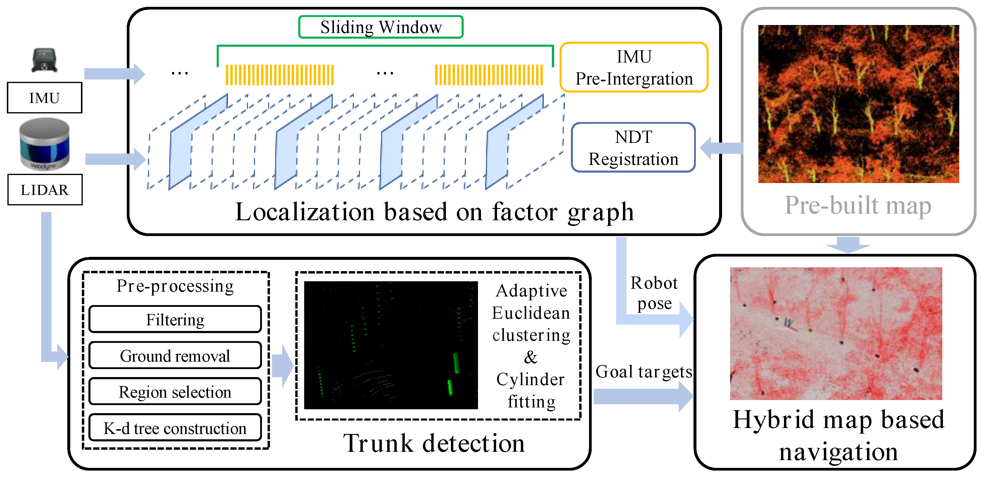
• A tightly coupled sliding window-based factor graph pose-tracking method for forest operation robots, especially rubber-tapping robots, providing stable and accurate 3D pose estimation continuously in forest scenarios;
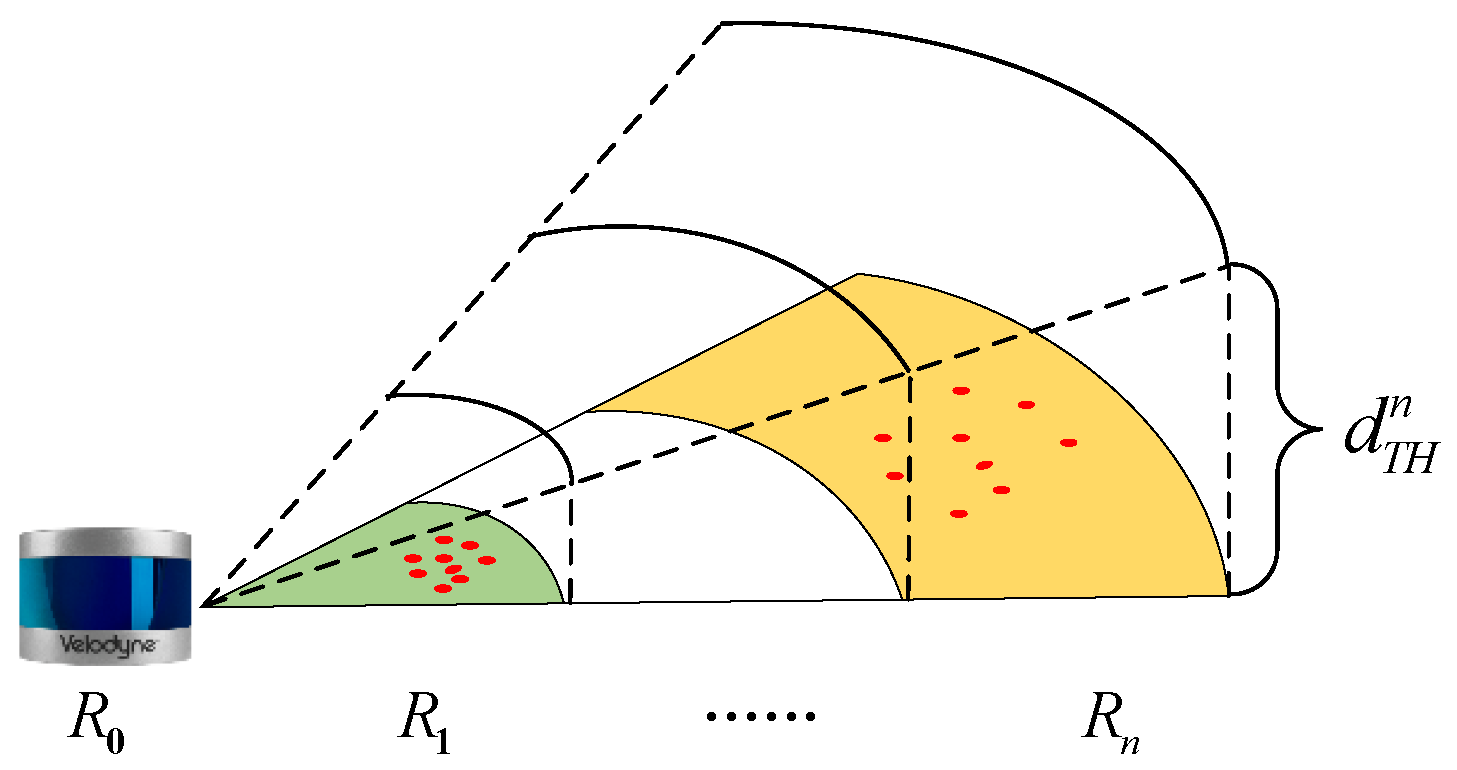
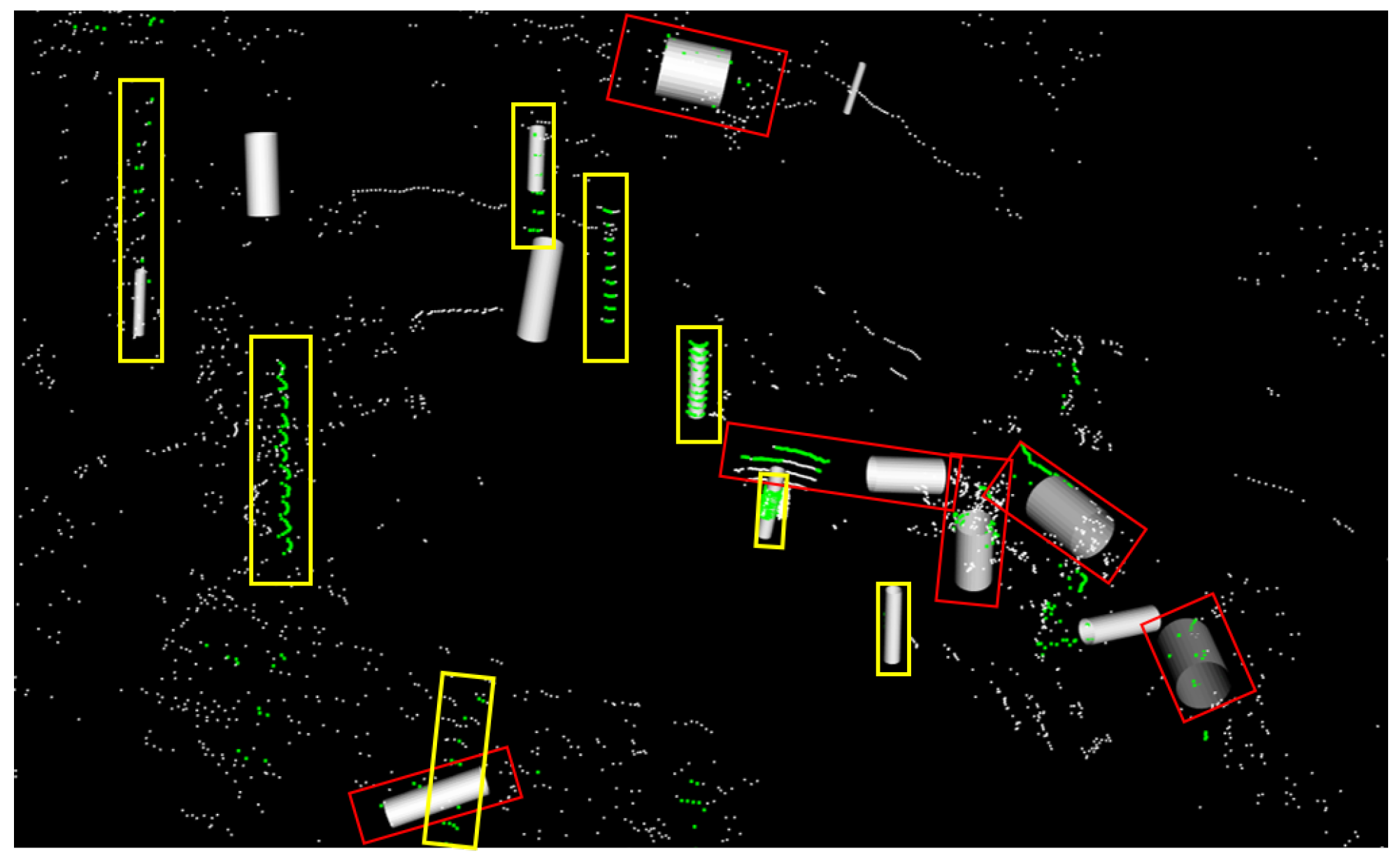
• A tree trunk detection method based on distance-adaptive Euclidean clustering, followed by cylinder fitting and a composite criteria screening, achieving a precision of 93.0% and a recall of 87.0% within the ROI;
• An active navigation system based on detected tree trunk guidance in hybrid map mode, which eliminates the need for manual target selection during navigation, improving efficiency;
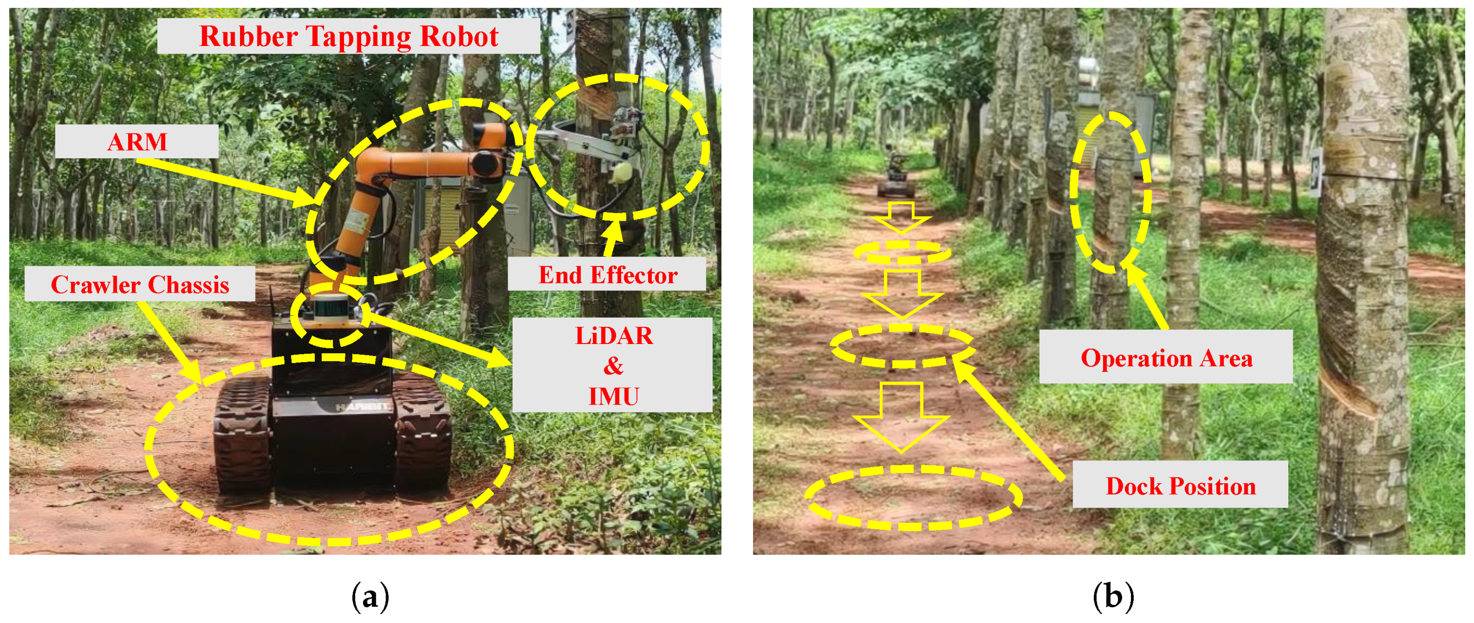
• A practical validation is completed in robot rubber-tapping tasks of a real rubber plantation.

2. Related Work

Previous studies identified two main automated alternatives to manual rubber tapping: trunk-affixed facilities and track-based systems [3,4]. However, these alternatives require a basic infrastructure and are impractical for the vast expanse of rubber forests worldwide. Therefore, mobile robots that can operate autonomously in the forests provide a more effective solution. Given that planning no longer presents a significant challenge for track-based robots, the precondition for active robotic navigation necessitates robust localization. Additionally, it requires the ability to detect reliable targets to serve as navigation points.

2.1. Localization

Localization primarily bifurcates into two parts, global localization and pose tracking, which are fundamental for forest robots to navigate. The global navigation satellite system (GNSS) is a common sensor used for outdoor localization, but it performs poorly in a rubber plantation due to the shading of the tree canopy. Visual-based methods are unsuitable for night time with insufficient textures. Therefore, 3D LIDAR is mainly relied on for pose tracking. The iterative closest point (ICP)-based method [5,6] can achieve accurate matching results in non-real-time applications. However, to improve real-time performance, point cloud line [7] or plane [8] features can be extracted for matching. Nevertheless, these methods are limited in the case of point cloud distortion or insignificant features. NDT, which uses a normal distribution to describe the local state of the point cloud instead of the raw point cloud, is more suitable for large-scale point cloud matching [9,10]. However, relying on LIDAR alone cannot guarantee the robustness of the pose estimation, so multi-sensor fusion localization is necessary. LOAM [11], LeGO-LOAM [12], and V-LOAM [13] are examples of loosely coupled methods that combine LIDAR and IMU measurements for better accuracy. With the maturity and application of IMU pre-integration theory, tightly coupled methods based on IMU pre-integration, such as LIOM [14] and LIO-SAM [15], can optimize LIDAR and IMU measurements jointly, achieving higher accuracy and real-time robot trajectory estimation.

For pose tracking, canonical sensor fusion strategies employed for conventional outdoor robots are generally classified into two categories: Bayesian filter-based methods and graph optimization-based methods. Bayesian filter-based methods, such as EKF, UKF, and PF, utilize kinematic assumptions and multi-sensor data to predict and correct the robot pose. EKF-based localization, as demonstrated by Wolcott et al. [16,17], is capable of attaining precision at the centimeter level on urban roads by constructing Gaussian mixture maps using LIDAR reflectivity and height data as observations. However, EKF-based methods may have larger errors in strongly nonlinear systems or inaccurate initial values. UKF, which avoids linearization errors by utilizing unscented transform (UT) and avoids solving the Jacobi matrix, was successfully applied by Koide et al. [18] to fuse the post-integration of IMU for state prediction and NDT for LIDAR with point cloud map alignment to complete robot 3D localization. Particle filter-based algorithms, which generate a large number of random particles to approximate the posterior distribution of the state by Monte Carlo methods for state estimation, can be applied to nonlinear systems and non-Gaussian distributions. Therefore, there has been significant research on particle filter-based localization [19,20,21,22,23,24]. However, particle filter-based methods are subject to particle degeneracy and sample impoverishment, which are significant limitations.

Graph optimization-based methods describe the robot’s poses and constraints by nodes and edges, making it easy to incorporate more observations into the optimization framework. One approach is to use landmarks and pose transformations in sparse graphs [25,26], which can ignore important data correlations. An alternative strategy involves the utilization of a sliding window, which serves to streamline the integration of unordered observations originating from multiple sources, while simultaneously reducing the quantity of constraints imposed. Merfel et al. proposed a sliding window pose graph [27,28] that enables efficient optimization and a new form of marginalization, which can adapt to available computing resources by adjusting the size of the sliding window. Ding et al. [29] proposed a LIDAR localization system based on a graph-optimized sensor fusion framework, which combines global matching and complementary information, such as LIDAR-inertial odometry, to achieve accurate and smooth localization estimation. Wilbers et al. [30] proposed a global prior approximating sliding window marginalization using a sparse graph approach that incorporates landmark information into the state estimation problem and uses the sliding window formulation to correct for data correlation [31]. As a non-random algorithm, graph optimization-based localization methods can achieve accurate and efficient results. With the help of the sliding window, it can also achieve real-time and robust localization. Therefore, graph optimization-based localization methods have become the mainstream approach [32].

2.2. Trunk Detection

Trunk detection requires point cloud segmentation (PCS) as a prerequisite. PCS involves dividing a point cloud into non-overlapping regions based on the geometry or spatial relationship of the points in the point cloud [33]. For a single LIDAR sweep, the point cloud describes the surface features of an object and points belonging to the same object are usually close in distance or share similar features. In scenarios where the surface is compounded with some geometry, the point cloud can be segmented by model fitting. Miadlicki K. et al. [34] utilized the RANSAC algorithm and dot product of vector for ground plane estimation and ground points filtration in a loader crane sensor fusion system. Himmelsbach, M. et al. [35] fit the point cloud that was dimensionally reduced with a straight line, and finally filtered the ground points by height information, which quickly segments the road points and points from other objects. Clustering-based PCS is suitable for the segmentation of irregularly shaped objects. Kenji Koide et al. [18] used a Euclidean distance-based clustering algorithm for people detection. Before clustering, points overlapping with environmental map points were removed. Haselich’s split–merge clustering algorithm was used to avoid wrongly merging clusters when they are close enough in distance. Nie, F. et al. [36] used density-based spatial clustering of applications with noise (DBSCAN) with density field correction to segment the LIDAR point cloud, aiming to reduce the effect of distance on the density of LIDAR points. Leveraging the formidable parallel computation prowess inherent in GPUs, Zhao et al. [37,38] introduced an innovative online seed optimization strategy aimed at accelerating the mean-shift algorithm. Remarkably, this approach engenders approximately a threefold increase in speed, a feat surpassing even the most sophisticated GPU-based clustering algorithms, while optimizing GPU memory utilization. Nonetheless, given the financial constraints and power-consumption considerations, the robots under consideration in this study are not equipped with GPUs. The methodologies delineated in [39,40] initially carry out 3D reconstruction to generate dense point clouds either through LIDAR SLAM or SFM (structure from motion), with trunk detection being subsequently conducted offline.

Capitalizing on the wealth of information provided by RGB cameras, tree trunk detection has gained considerable traction within the realm of computer vision. Zheng et al. [41] introduced a lightweight attention Ghost-HRNet (AGHRNet) predicated on deep learning, geared towards differentiating between the trunk and branches of trees and the complex background of the orchard. Concurrently, the burgeoning availability of cost-effective RGB-D sensors has stimulated interest in RGB-D-based object reconstruction [42] and tracking methodologies [43]. By enhancing the YOLOV5 framework, Su et al. [44] enhanced tree trunk detection across a spectrum of seasonal conditions, with the position of targets being determined on the basis of depth data. However, in the working scenarios of rubber-tapping robots, these machines operate at night, rendering them unsuitable for trunk detection algorithms based on RGB images. Furthermore, the inter-tree spacing of rubber trees reaches up to 6 meters, exceeding the depth estimation range provided by commercial RGB-D sensors. Consequently, the effective deployment of these sensors on the rubber-tapping robots under study presents formidable challenges. On the other hand, thermal sensors, which measure object temperature and emitted heat, have demonstrated the potential in circumventing the lighting sensitivity issue associated with conventional RGB cameras. In the specific domain of rubber tapping, thermal sensors have realized commendable results in trunk detection [45] and the defect detection of trunks [46]. However, akin to conventional RGB cameras, the accuracy of depth prediction remains a weak link, and the detection results cannot be directly employed for target point navigation.

3. Materials and Methods

As depicted in Figure 2, in order to facilitate the active navigation of rubber-tapping robots based on a hybrid map model, we primarily address two challenges: pose tracking and tree trunk detection. Mapping is not included, as this can be completed offline without incurring additional costs. In the pose-tracking part, factors are obtained from the LIDAR data using NDT registration, IMU pre-integration, and sliding window marginalization. After local optimization within the time window, the robot’s pose is used for motion planning during navigation. In the trunk detection part, the LIDAR data are pre-processed to remove invalid points, increasing the efficiency of the search. Distance-adaptive Euclidean clustering and cylinder fitting are used to obtain clusters that conform to the trunk characteristics, which are used as navigation targets. For hybrid map-based navigation, beyond its usage for localization, a pre-constructed 3D point cloud map also facilitates the generation of a 2D grid map, which serves a crucial role in planning. The system selects detected trunks as navigation targets based on a specific strategy.

3.1. Pose Tracking Based on Factor Graph

The graph optimization-based approach outperforms the filter-based approach in terms of localization accuracy. Unlike the strict requirement for global constraints in SLAM, pure localization only requires constraints on a local scale, and new observations have little effect on the historical information. Incremental optimization transforms the factor graph into a Bayesian network and further constructs a Bayesian tree, making efficient incremental updates and inferences possible so that new observations fusion and robot state online updating can be performed at any time [47]. Therefore, we use the scan-to-map method based on NDT [9,48] to estimate the robot state transition, which fuses the IMU pre-integration factor and uses a factor graph optimization model based on incremental updates to incrementally optimize the local odometry and estimate the robot pose to ensure real time and accuracy.

Within the context of pose tracking, the robot’s pose, denoted as $\mathcal{X}$, is defined as the state, while $\mathcal{Z}$ represents the observation. The estimation of robot states and trajectories using observations from different sensors can be expressed as a maximum a posteriori (MAP) problem as shown in Formula (1):

$${\mathcal{X}}^{*}=\underset{\mathcal{X}}{argmax}P(\mathcal{X}\mid \mathcal{Z})$$

(1)

Usually, pose estimation is to find the MAP solution ${\mathcal{X}}^{*}$, which maximizes the probability $P(\mathcal{X}\mid \mathcal{Z})$ of state $\mathcal{X}$ and measurement $\mathcal{Z}$. The measurements in this paper include 3D LIDAR, IMU, and camera, so $P(\mathcal{X}\mid \mathcal{Z})$ can be decomposed into Formula (2):

$$P(\mathcal{X}\mid \mathcal{Z})\propto \underset{\mathcal{X}}{argmax}\prod _{t,s}P\left({\mathbf{z}}_t^I\mid {\mathbf{x}}_t^L,{\mathbf{x}}_{t-1}^L\right)\prod _{t}P\left({\mathbf{z}}_t^{\mathrm{G}}\mid {\mathbf{x}}_t^{\mathrm{f}},{\mathbf{x}}_{t-1}^G\right)$$

(2)

State $\mathcal{X}$ represents the pose of the robot $[x_1,\cdots ,x_N]$, and the number of poses T defines the size of the sliding window. Assuming that the measurement noise is mutually independent and obeys a Gaussian distribution with zero means, the optimization problem is equivalent to minimizing the sum of cost functions as shown in Equation (3):

$${\mathcal{X}}^{*}=\underset{\mathcal{X}}{argmin}\sum {\mathit{e}}_k{\left(\mathit{x},{\mathit{z}}_k\right)}^{\top }{\mathbf{\Omega }}_k{\mathit{e}}_k\left(\mathit{x},{\mathit{z}}_k\right)$$

(3)

The term $\left(\mathit{x},{\mathit{z}}_k\right)$ symbolizes the cost error function between the measurement ${\mathit{z}}_k$ and the state vector x. Concurrently, ${\mathbf{\Omega }}_k$ signifies the corresponding information matrix. Since the localization process includes three measurements as well as prior factors generated by the marginalization process, the cost function can be expanded as shown in Equation (4):

$$\begin{array}{cc}\hfill {\mathcal{X}}^{*}=\underset{\mathcal{X}}{argmin}& \sum _i{\mathrm{e}}^{\mathrm{map}}{\left({\mathit{x}}^{\mathrm{P}},{\mathit{z}}_i^{\mathrm{map}}\right)}^{\top }{\Omega }_i^{\mathrm{map}}{\mathrm{e}}^{\mathrm{map}}\left({\mathit{x}}^{\mathrm{P}},{\mathit{z}}_i^{\mathrm{map}}\right)\hfill \\ \hfill & +\sum _i{\mathrm{e}}^{\mathrm{imu}}{\left({\mathit{x}}^{\mathrm{P}},{\mathit{z}}_i^{\mathrm{imu}}\right)}^{\top }{\Omega }_i^{\mathrm{imu}}{\mathrm{e}}^{\mathrm{imu}}\left({\mathit{x}}^{\mathrm{P}},{\mathit{z}}_i^{\mathrm{imu}}\right)\hfill \\ \hfill & +F^{marg}\left(\mathit{x}\right)\hfill \end{array}$$

(4)

The superscript map denotes the measurement cost function obtained by NDT between the LIDAR point cloud and point cloud map, the superscript imu denotes the pre-integration cost function between two LIDAR point clouds, and $F^{marg}\left(\mathit{x}\right)$ denotes the measurement cost of sliding window marginalization. Finally the optimal value ${\mathcal{X}}^{*}$ is obtained by iterative optimization of ${\mathcal{X}}^{*}=-\mathit{b}$ by the factor graph optimization method. $\mathit{H}$ and $\mathit{b}$ are shown in Equation (5), and ${\mathit{J}}_i$ is the Jacobian matrix of the cost function at $\mathcal{X}$:

$$\begin{array}{cc}\hfill \mathit{H}& =\sum _i{\mathit{J}}_i^{\top }{\mathbf{\Omega }}_i{\mathit{J}}_i\hfill \\ \hfill \mathit{b}& =\sum _i{\mathit{J}}_i^{\top }{\mathbf{\Omega }}_i{\mathbf{e}}_i\hfill \end{array}$$

(5)

With factor graph as the core architecture, data fusion through Bayesian tree-based incremental inference can effectively deal with the asynchrony and delay in sensor measurements. The pose of each point cloud frame is obtained through factor graph optimization, and then converted to the robot coordinate according to the extrinsic parameters as the basis for robot navigation. When inserting new nodes, the factor graph is optimized by incremental smoothing and Bayesian tree inference. Therefore, NDT measurement factors, IMU pre-integration factors and prior factors generated by sliding window marginalization are introduced in this paper for local state estimation. Meanwhile, all measurement noises are assumed to obey Gaussian distribution. The factor graph is shown in Figure 3.

NDT measurement factor: NDT is used to register the current point cloud with the pre-built 3D point cloud map. NDT is represented by a combination of normal distributions describing the probability of finding a surface point at a certain location, instead of single points in the ICP algorithm. The normal distribution gives a piecewise smooth representation of the point cloud with continuous first and second derivatives. Using this representation, standard numerical optimization methods can be applied for point cloud registration. Since the points are not directly used for matching, there is no need for the nearest neighbor search in the loop, which has heavy computational cost, like the ICP algorithm. The algorithm keeps the NDT representation of the point cloud rather than the raw point cloud in the memory, which reduces memory cost and is very conducive to matching with a large-scale point cloud.

The algorithm first divides the 3D point cloud map into cube cells with a specific size. When the number of points in a cell exceeds a certain threshold, calculate the average $\overrightarrow{\mu }$ and covariance matrix $\Sigma$ of the cell as shown in Equation (6):

$$\begin{array}{c}\begin{array}{cc}\hfill \overrightarrow{\mathit{\mu }}& =\frac{1}{m}\sum _{k=1}^m{\overrightarrow{\mathit{x}}}_k\hfill \\ \hfill \Sigma & =\frac{1}{m-1}\sum _{k=1}^m\left({\overrightarrow{\mathit{x}}}_k-\overrightarrow{\mathit{\mu }}\right){\left({\overrightarrow{\mathit{x}}}_k-\overrightarrow{\mathit{\mu }}\right)}^{\mathrm{T}}\hfill \end{array}\hfill \end{array}$$

(6)

${\overrightarrow{\mathit{x}}}_k(k=1,\dots ,m)$ represents the point cloud in the cube cell. Use Gaussian distribution $\mathcal{N}(\overrightarrow{\mathit{\mu }},\Sigma )$ to model the point at $\overrightarrow{x}$ in each unit, as shown in Equation (7):

$$p(\overrightarrow{x})=\frac{1}{{\left(2\pi \right)}^{D/2}\sqrt{|\Sigma |}}exp\left(-\frac{{(\overrightarrow{x}-\overrightarrow{\mu })}^{\mathrm{T}}{\Sigma }^{-1}(\overrightarrow{x}-\overrightarrow{\mu })}{2}\right)$$

(7)

The rotation and translation of the current pose estimation, which is to be optimized, can be represented by the vector $\mathbf{p}=\left[t_x,t_y,t_z,{\phi }_x,{\phi }_y,{\phi }_z\right]$, where $t_x$, $t_y$, and $t_z$ represent the translation in the x, y, and z directions, and ${\phi }_x$, ${\phi }_y$, and ${\phi }_z$ represent the Euler angles of the rotation about the three axes. The algorithm calculates how well the poses match by evaluating the PDF at all points in a single LIDAR sweep. The optimization problem can usually be transformed into the minimization problem of the object function, so the cost function can be defined as negative to minimize the cost of the most appropriate pose estimation. Given a set of points $\mathcal{X}=\left\{{\mathbf{x}}_1,\dots ,{\mathbf{x}}_n\right\}$ and pose $\mathbf{p}$, the point cloud poses are transformed by the transformation matrix $T(\mathbf{p},x_k)$, and the cost function of this transformation is shown in Equation (8):

$$s\left(\mathbf{p}\right)=-\sum _{k=1}^{n}p\left(T\left(\mathbf{p},{\mathbf{x}}_k\right)\right)$$

(8)

In the process of 3D point cloud registration, $t(\mathbf{P},x)$ is expressed as Formula (9), where $c_i=cos{\phi }_i$, $s_i=sin{\phi }_i$, such as $s_x=sin{\phi }_x$:

$$T(\mathbf{p},x)={\mathbf{R}}_x{\mathbf{R}}_y{\mathbf{R}}_{z}x+t=\left[\begin{array}{ccc}{c}_y{c}_z& -c_y{s}_z& s_y\\ c_x{s}_z+s_x{s}_y{c}_z& c_x{c}_z-s_x{s}_y{s}_z& -s_x{c}_y\\ s_x{s}_z-c_x{s}_y{c}_z& c_x{s}_y{s}_z+s_x{c}_z& c_x{c}_y\end{array}\right]\overrightarrow{x}+\left[\begin{array}{c}{t}_x\\ t_y\\ t_z\end{array}\right]$$

(9)

Given the transformation matrix $\mathbf{P}$, the equation $H\Delta \mathbf{P}$= $-G$ can be solved iteratively by the Gaussian–Newton method, where H and G are the Hessian matrix and gradient of S. The increment $\Delta \mathbf{p}$ is superimposed to the estimated parameters of each iteration. Let ${\mathbf{x}}^{\prime }\equiv t(\mathbf{P},\mathbf{x})-\mathbf{Q}$, and ${\mathbf{x}}^{\prime }$ can be considered the transformation of x relative to the distribution center of the cell to which it belongs. The partial derivatives required by the equation can be obtained by the Jacobian matrix and the Hessian matrix. When $\Delta \mathbf{P}$ is less than the threshold, the algorithm is considered convergent and the final transformation matrix $\mathbf{P}$ is obtained; otherwise, the iteration is continued until convergence. After convergence, the obtained $\mathbf{P}$ is added to the factor graph as a measurement factor. Due to the application of incremental optimization and the sliding window method, the algorithm fully meets the demand for real-time performance. Meanwhile, the accuracy of localization is ensured by calculating the NDT measurement factors between all LIDAR point clouds (20 fps) and the prior map.

IMU Pre-integration factor: Firstly, the observation model of IMU is established as shown in Formula (10), of which $a_m^B$ and ${\omega }_m^B$ are the observed values of acceleration and angular velocity in the IMU carrier coordinate system, ${}^{W}g$ represents the gravity vector in world coordinate system, ${}^{W}a$ and ${}^W\omega$ represent the real values of acceleration and angular velocity in world coordinate system, and $q_{BW}$ is the quaternion representation of IMU carrier transformation relative to the world coordinate system:

$$\begin{array}{c}{a}_m^B=q_{BW}\left({}^{W}a+{}^{W}g\right)+b_a+n_a\hfill \\ {\omega }_m^B={}^W\omega +b_g+n_g\hfill \end{array}$$

(10)

The measurement information of IMU is obtained in the carrier coordinate system. Theoretically, the real acceleration ${}^{W}a$ is offset by acceleration $b_a$ and noise $n_a$, and their sum constitutes the final acceleration measurement $a_m^B$. Similarly, the angular velocity ${}^w\Omega$ is biased by the gyroscope $b_g$ and noise $n_g$, and their sum constitutes the final angular velocity measurement ${\omega }_m^B$ and noise $n_a$, and $n_g$ obeys the Gaussian distribution. The derivative of PVQ to time is as shown in Equation (11):

$$\begin{array}{c}{\dot{\mathbf{p}}}_{w{b}_t}={\mathbf{v}}_t^w\hfill \\ {\dot{\mathbf{v}}}_t^w={\mathbf{a}}_t^w\hfill \\ {\dot{\mathbf{q}}}_{b_t}^w={\mathbf{q}}_{b_t}^w\otimes \left[\begin{array}{c}0\\ \frac{1}{2}{\omega }^{b_t}\end{array}\right]\hfill \end{array}$$

(11)

For two consecutive keyframes ${\mathbf{f}}_i$ and ${\mathbf{f}}_j$, their corresponding moments are I and J. According to the post-integration, the position, speed, and rotation at time J can be obtained by integrating the measured values of IMU from those of the system at time I as shown in Formula (12):

$$\begin{array}{c}{\mathbf{p}}_{b_j}^w={\mathbf{p}}_{b_i}^w+{\mathbf{v}}_{b_i}^w\Delta t_{ij}+{\int \int }_{t\in [i,j]}\left({\mathbf{q}}_{b_t}^w\left({\mathbf{a}}^{b_t}-b_a-n_a\right)-{\mathbf{g}}^w\right)d{t}^2\hfill \\ {\mathbf{v}}_{b_j}^w={\mathbf{v}}_{b_i}^w+{\int }_{t[i,j]}\left({\mathbf{q}}_{b_t}^w\left(a_m^B-b_a-n_a\right)-{\mathbf{g}}^w\right)dt\hfill \\ {\mathbf{q}}_{b_j}^w={\mathbf{q}}_{b_i}^w\otimes {\int }_{t[i,j]}\frac{1}{2}{\mathbf{q}}_{b_t}^w\otimes \left({\omega }_m^B-b_g-n_g\right)dt\hfill \end{array}$$

(12)

where $\Delta t$ represents the time interval of IMU update, and ${\mathbf{q}}_{b_t}^w$ is the quaternion representation of the rotation of the body coordinate system relative to the world coordinate system at time t. According to Formula (12), when obtaining ${\mathbf{p}}_{b_j}^w$, ${\mathbf{v}}_{b_j}^w$, ${\mathbf{q}}_{b_j}^w$ of the system at time j, the corresponding starting state at time i must be known. When the initial state changes, Formula (12) needs to be reintegrated. In optimization-based state estimation, it is necessary to re-compute the integration after every optimization update of ${\mathbf{q}}_{b_t}^w$. Frequent integral calculation wastes a lot of computing resources.

The idea of IMU pre-integration is to adjust the reference coordinate system from the world coordinate system to the body coordinate system of the keyframe at time i. The integral term in the PVQ integration formula becomes the pose relative to the body coordinate system at time i rather than the pose relative to the world coordinate system as shown in Formula (13):

$$\begin{array}{c}{\mathbf{p}}_{w{b}_j}={\mathbf{p}}_{w{b}_i}+{\mathbf{v}}_i^w\Delta t-\frac{1}{2}{\mathbf{g}}^w\Delta t^2+{\mathbf{q}}_{w{b}_i}{\int \int }_{t\in [i,j]}\left({\mathbf{q}}_{b_i{b}_t}{\mathbf{a}}^{b_t}\right)d{t}^2\hfill \\ {\mathbf{v}}_j^w={\mathbf{v}}_i^w-{\mathbf{g}}^w\Delta t+{\mathbf{q}}_{w{b}_i}{\int }_{t\in [i,j]}\left({\mathbf{q}}_{b,b_t}{\mathbf{a}}^{b_t}\right)dt\hfill \\ {\mathbf{q}}_{w{b}_j}={\mathbf{q}}_{w{b}_i}{\int }_{t\in [i,j]}{\mathbf{q}}_{b_i{b}_t}\otimes \left[\begin{array}{c}0\\ \frac{1}{2}{\mathit{\omega }}^{b_t}\end{array}\right]dt\hfill \end{array}$$

(13)

The pre-integration component is defined as shown in Formula (14). The pre-integration model assumes that the integration term in a short time is constant and the state value of the keyframe is a variable. The IMU pre-integration measurement has nothing to do with the position, speed, and direction of the IMU but only with the initial state of the IMU associated with the key frame:

$$\begin{array}{c}\Delta {\mathbf{p}}_{ij}={\int \int }_{t\in [i,j]}\left({\mathbf{q}}_{b_i{b}_t}{\mathbf{a}}^{b_t}\right)d{t}^2\\ \Delta {\mathbf{v}}_{ij}={\int }_{t\in [i,j]}\left({\mathbf{q}}_{b_i{b}_t}{\mathbf{a}}^{b_t}\right)dt\\ \Delta {\mathbf{q}}_{ij}={\int }_{t\in [i,j]}{\mathbf{q}}_{b_i{b}_t}\otimes \left[\begin{array}{c}0\\ \frac{1}{2}{\mathit{\omega }}^{b_t}\end{array}\right]dt\end{array}$$

(14)

In this way, the IMU data over a period of time are directly integrated to obtain the pre-integration. The IMU pre-integration item between the key frame ${\mathbf{F}}_i$ and ${\mathbf{F}}_j$ is taken as a constant so that there is no need to repeat the process of integration, even if the state changes during the optimization process. Upon procuring the result of the pre-integration, the pre-integration term is incorporated to compute the state transformation between keyframes as delineated in Formula (15). Subsequently, this transformation is appended to the constraints of the factor graph as an incremental factor:

$$\left[\begin{array}{c}{\mathbf{p}}_{w{b}_j}\\ {\mathbf{v}}_j^w\\ {\mathbf{q}}_{w{b}_j}\end{array}\right]=\left[\begin{array}{c}{\mathbf{p}}_{w{b}_i}+{\mathbf{v}}_i^w\Delta t-\frac{1}{2}{\mathbf{g}}^w\Delta t^2+{\mathbf{q}}_{w{b}_i}\Delta {\mathbf{p}}_{ij}\\ {\mathbf{v}}_i^w-{\mathbf{g}}^w\Delta t+{\mathbf{q}}_{w{b}_i}\Delta {\mathbf{v}}_{ij}\\ {\mathbf{q}}_{w{b}_1}\Delta {\mathbf{p}}_{ij}\end{array}\right]$$

(15)

Prior factor obtained by marginalization in sliding window: The purpose is to marginalize the old pose constraint and add a new one to the factor graph so as to ensure a constant number of pose constraints. Eliminating a variable $x_j$ and its associated factors is equivalent to marginalizing a variable from the full probability distribution, which has an expensive cost, and the incremental updating based on the Bayesian tree makes the marginalization easier. Due to the characteristics of the Bayesian tree, the variable $x_n$ in the leaf cluster can be easily marginalized. As shown in Equation (16), the integration of $x_n$ can be performed only from the end conditions of the joint distribution. By using time variable ordering in the elimination step, the oldest variable in the factor graph can be ensured to appear in the leaf cluster:

$$\begin{array}{cc}\hfill p\left(x_1\dots x_{n-1}\right)=& {\int }_{x_n}p\left({\theta }_1\right)p\left(x_2\mid x_1\right)\dots \dots p\left(x_{n-1}\mid x_1\dots x_{n-2}\right)p\left(x_n\mid x_1\dots x_{n-1}\right)\hfill \\ \hfill =& p\left(x_1\right)p\left(x_2\mid x_1\right)\dots p\left(x_{n-1}\mid x_1\dots x_{n-2}\right)\hfill \end{array}$$

(16)

While it is easy to marginalize in the decomposition Bayesian tree structure, it is necessary to modify the nonlinear system to allow the re-linearization and nonlinear optimization of the remaining variables. All the original nonlinear factors used to construct the Bayesian tree involving marginal variables must be deleted, and the information contained in these factors which are about the variables still in the sliding window must be inserted. The incremental updating process edits the leaf clusters of the Bayesian tree and inserts the factors calculated in the previous variable elimination step. By caching these factors in the elimination process, they do not need to be recalculated in the process of marginalization, ensuring the real-time update [49].

3.2. Trunk Detection

Point cloud pre-processing: The input of the trunk detection phase is a 3D LIDAR point cloud $P=\left\{p_i\right|p_i=(x_i,y_i,z_i)\in {\mathbb{R}}^3,i=1,\dots ,I\}$, where I is the total number of points in a single scan. The point cloud pre-processing leaves a subset $P^{*}$ for clustering. (a) Statistical filter. In a rubber plantation, there are stable features that we need such as the trunks and ground, and there are many unstable features that generate noise points, such as weeds and leaves. The noise points are significantly different from the point clouds formed by continuous surfaces. Therefore, we applied a statistical filter to remove significant stand-alone noise points, reducing incorrect clustering due to unstable features. (b) Ground points removal. The ground points around the robot show a dense and regular arrangement, which usually causes meaningless clustering. Therefore, we select the points near the ground with $|z_i-h_{LIDAR}|<d_{TH}$, and use RANSAC to fit the plane to obtain the ground points. Then the ground points are removed from the point cloud. (c) Region of interest (ROI) selection. The clustering of 3D points can be computationally intensive, whereas down-sampling can easily lead to the points in the ROI being reduced indiscriminately, resulting in clustering and fitting problems. In practice, more points are filtered out because they do not provide clear information or they are in a region of no interest, which substantially reduces the size of the point cloud that needs to be clustered. Possible reasons for filtering include being too sparse (Figure 4) or regions lying outside the robot’s passable area. (d) K-d tree construction. In our system, the k-nearest neighbors are queried with Euclidean clustering. A k-d tree is applied to accelerate the search for the k-nearest neighbors. To accelerate the clustering process, a k-d tree is built for every frame of the LIDAR observation.

Clustering with distance threshold correction: In our system, we use a distance-adaptive Euclidean clustering method to extract trunks from LIDAR observation. Because of the distance effect of 3D LIDAR, the shape and density of the point cloud vary significantly with the distance and the relative position between the trunks and the sensor as shown in Figure 4. Due to the vertical angular resolution of the LIDAR ($\Delta \theta =2^{\circ }$), the vertical distance of the consecutive points increases with distance, as shown in Equation (17), where $d_V$ means the vertical distance between two LIDAR lines and $d_H$ means the horizontal distance from the sensor:

$$d_V=d_H·|tan{\theta }_{i+1}-tan{\theta }_i|,i=1,\dots ,16$$

(17)

Therefore, a constant distance threshold will result in observation points from a distant tree not being clustered correctly. Inspired by the cluster algorithm [50], we correct the threshold $d_{TH}$ based on scan range r as follows:

$$d_{TH}=2·r·tan\frac{\Delta \theta }{2}$$

(18)

For straight vertical objects, such as trunks, when the distance between two adjacent lines is less than this threshold, the clustering criteria can be satisfied. The horizontal distance is not considered here because the horizontal resolution is much smaller than the vertical. However, the longer the maximum scan range, the higher the value of $d_{TH}$, and therefore, the number of points falling within the same cluster, even if they are not from a single trunk. To reduce the complexity, the horizontal space is divided into nested circular regions around the sensor, and a constant threshold is calculated for every annular region as shown in Figure 5.

Cylinder fitting and trunk screening: After clustering, point clouds in different clusters are judged as to whether they are from tree trunks or not. The geometric feature of a trunk is similar to a cylinder, so we assume that the trunk is a cylinder, then fit the corresponding cylindrical model of the point cloud by the least squares method, and evaluate whether it is a tree according to the DBH, location, orientation, and other indicators. If it is a tree, the projected position of the central axis in the horizontal plane is used as the target for robot navigation.

For the purpose of obtaining the most similar cylinder model to the point cloud, in the fitting process, we use the cylindrical surface function as the objective function [51] as shown in Equation (19):

$$\left[\begin{array}{c}x\hfill \\ y\hfill \\ z\hfill \\ a\hfill \\ b\hfill \\ c\hfill \\ r\hfill \end{array}\right]\begin{array}{cc}& =\underset{x,y,z,a,b,c,r}{argmin}\delta \hfill \\ \hfill & =\underset{x,y,z,a,b,c,r}{argmin}\sum _{i=0}^n\parallel {(x-x_i)}^2+{(y-y_i)}^2+{(z-z_i)}^2\hfill \\ \\ & -{[a(x-x_i)+b(y-y_i)+c(z-z_i)]}^2-r^2{\parallel }_2\hfill \end{array}$$

(19)

$(x,y,z)$ is the central position of the cylinder, $(a,b,c)$ is the vector of the central axis, $(x_i,y_i,z_i)$ is any point on the cylinder surface, and r is the radius of the cylinder. When dealing with point clouds, the distances between the points and the cylindrical surface are used as the residual block, and they are added together to become the objective function. The distance term is generated for every point in the cluster. The radius of the cylinder and position of the central axis are adjusted so as to minimize the function. For the optimization convergence to be faster, we give the optimizer an approximate initial value. As shown in Equation (20), the initialization of the trunk center position $(x_0,y_0,z_0)$ gives the centroid of the cluster, and the vector of the central axis $(a_0,b_0,c_0)$ is given since the trunk is almost perpendicular to the ground. Since the DBH of rubber trees in the same rubber plantation will be within a certain range, we can estimate an empirical average radius $r_0$ as the initial value of the cylinder radius:

$$\begin{array}{cc}\hfill \left[\begin{array}{c}{x}_0\\ y_0\\ z_0\end{array}\right]=\sum _{i=0}^n\left[\begin{array}{c}{x}_i\\ y_i\\ z_i\end{array}\right]/n,\left[\begin{array}{c}{a}_0\hfill \\ b_0\hfill \\ c_0\hfill \end{array}\right]& =\left[\begin{array}{c}0\hfill \\ 0\hfill \\ 1\hfill \end{array}\right]\hfill \end{array}$$

(20)

The radius r obtained from the optimization results varies with the shape of the point cloud cluster. Some point cloud clusters which do not belong to any trunks may fit particularly large or small cylinders with small residuals. Since we have the DBH range (10–20 cm in our experimental area) and orientation range as a strong prior hypothesis in advance, we can determine whether the point cloud cluster belongs to a trunk or not based on the obtained cylinder radius and central axis orientation.

To avoid outlier interference, RANSAC is used first to fit a part of the point cloud [52,53], and other points are judged as to whether or not they are inliers according to the fitting results. When the number of inliers is greater than the threshold and the radius is within the range, we consider the that the point cloud cluster belongs to the trunk and use the mean value of the inliers’ location as the trunk centroid to avoid the outliers leading to the missed detection of the trunk. The results of the detection are shown in Figure 6.

3.3. Hybrid Map Navigation

The hybrid map refers to navigating using a 3D point cloud map for localization and motion planning using a 2D probabilistic grid map. Three-dimensional matching based on a point cloud map can better cope with the cases of lacking features and improve the accuracy and reliability of robot localization in complex environments. Also, the use of 2D probabilistic maps for ground mobile robot navigation is well established and can reduce the complexity of motion-planning algorithms. For security reasons, we choose to project the point cloud between the ground and the height of the upper surface of the chassis on the ground to obtain a 2D map. With the points identified corresponding to the tree trunks in Section 3.2, we calculate the centroid of each cluster and project the centroid onto the ground plane to obtain a 2D coordinate that can be the goal of robot navigation. Projecting the centroid onto the ground plane simplifies the navigation task by reducing the dimensionality of the problem, providing a clear goal point for the robot to move towards. By obtaining the trunk position as a goal pose reference, we choose the nearest tree in front of the robot as the next navigation target when docking at the current tree. The subsequent phase of the process entails the execution of path planning, utilizing the A* algorithm. This is then followed by the implementation of the timed elastic band (TEB) [54] technique for meticulous motion planning.

4. Results

In order to evaluate the proposed method, a series of experiments were conducted, and field validation was carried out on a rubber-tapping robot. The robot utilized an electric crawler chassis and an AUBO-i5 6-DOF collaborative manipulator to operate the end effector for rubber tapping. For robot navigation, a VLP-16 3D LIDAR and a Hi216 6-axis IMU module integrated with a MPU-6050 chip were employed as sensors. The platform and sensors used in the experiments are illustrated in Figure 1a. The dataset used was collected from a real rubber plantation, which included several ramps and curves. Since obtaining ground truth was not feasible in the given environment, a point cloud map and trajectory were obtained by running FAST-LIO2 offline with higher parameters as preparation and relative ground truth. The dataset experiments were conducted on a PC with an Intel Core i5-1135G7 processor, while the field validation was carried out using the robot-equipped computer with an Intel Core i7-7500U processor.

4.1. Pose Tracking

The overall performance of our proposed method in a real rubber plantation is presented in this experiment. The dataset was collected from a 30 m × 70 m area in size, containing the common terrains in a typical rubber plantation. To facilitate alignment of the trajectories when evaluating the algorithm, we used all 7993 frames of data in the dataset. The complete trajectories output by our proposed method as well as other pose-tracking algorithms on the dataset are shown in Figure 7. The movement of our robot starts from A and ends at D, turning at positions B and C to pass the ditches. Results show that our pose-tracking algorithm achieves generally better performance than algorithms based on UKF, MCL, and NDT-only.

As shown in Figure 7, the trajectories of all four methods are generally consistent with the ground truth in terms of trend. Intuitively, compared with other algorithms, trajectories obtained by the proposed method and UKF are closer to the ground truth. When the robot turns sharply or the terrain changes, the poses are estimated by NDT drift. MCL has the worst performance due to the fact that the odometry prediction it relies on will be seriously affected by wheel slipping. Without an odometry provided, the MCL-based algorithm invalidates entirely after passing the straight path from A to B. Figure 8 shows a clearer result of the trajectory comparison in the x, y, and z directions, and the aerial view.

As shown in Figure 8a, our method and the algorithm based on UKF outperform the localization algorithms based on MCL and NDT-only in all three directions. Figure 8b–e clearly show the output trajectories compared to the ground truth. In the algorithm with the UKF back-end, IMU data are used to derive the state prediction for the current moment based on the state at the previous moment. In the proposed algorithm, we use IMU pre-integration as constraints in the factor graph. This avoids the trajectory from producing abrupt changes at some places (position B and position C) due to incorrect estimation.

To quantitatively evaluate the localization accuracy of our algorithm, we carry out a further error analysis experiment. We calculated the absolute pose error (APE) and relative pose error (RPE) of every trajectory. The quantitative results on APE and RPE are shown in

Table 1. Quantitative results on absolute pose error (m).

Methods	Max	Mean	Min	Rmse	Std
Ours	0.464941	0.306398	0.128458	0.308381	0.034919
UKF	0.430175	0.325414	0.140065	0.327407	0.036074
MCL	4.411130	1.851616	0.029355	2.064198	0.912376
NDT	6.217928	0.532878	0.055203	0.983322	0.826416

and

Table 2. Quantitative results on relative pose error (m).

Methods	Max	Mean	Min	Rmse	Std
Ours	0.032788	0.006511	0.000332	0.007258	0.003208
UKF	0.053262	0.007903	0.000348	0.008789	0.003845
MCL	1.062193	0.032857	0.001063	0.064827	0.055883
NDT	1.053219	0.012379	0.000068	0.031304	0.028753

.

Table 1 shows that we achieve a global localization with a pose error of not more than 0.47 m and about 0.3 m on average, which indicates good consistency of the global trajectory. The minimum and maximum of APE are not statistically significant because of the strong randomness, especially when the values are scattered in a small interval. Table 2 indicates the accuracy of local pose estimation. Our approach outperforms the other methods in terms of quantitative metrics due to the sensor fusion as well as utilizing more historical state information, which effectively reduces the impact of the error estimations and makes the trajectory smoother. The correspondence of APE and RPE to the frame index is shown in Figure 9. It can be found that at indexes of 1000–1500 and 4000–4500, each algorithm has a tendency to increase the error to different degrees, which exactly corresponds to the robot’s sharp turns and terrain changes, indicating the challenge for pose estimation in the woods.

4.2. Trunk Detection

To evaluate our tree trunk detection algorithm, we selected the LIDAR frames of the robot at 10 locations where the target needs to be generated and manually tagged the tree trunks in the region of the LIDAR frame. Note that because the trees in the rubber forest are densely planted, a LIDAR frame may contain point clouds from up to 30 trees, but the trees in the distance are meaningless for the rubber-tapping robot’s selected navigation goal. Due to the ditch between the two lines of trees, the robot can only turn to another line at limited positions. So the most potential targets are in an area in front of the robot, and a few are on adjacent lines only when the robot needs to change operating areas. In this section, the region of interest includes the line where the robot is located and the adjacent lines on either side, four trunks in front of the robot, roughly within a 12 m in width and 8 m in length area with the robot chassis coordinate as the origin. As shown in Figure 10a, the distance between two adjacent lines of trees is about 6 m.

We conducted an evaluation of the performance and efficiency of tree trunk detection. For the performance evaluation, we evaluated the precision and recall of the detection algorithm through the measurement of true positives (TP), false positives (FP), and false negatives (FN). In this context, these metrics respectively correspond to the correctly identified trees, erroneously detected trees, and undetected trees, respectively. In terms of efficiency, we assessed it based on the number of frames processed per second (FPS), which was calculated from the time taken to process a single frame. In our algorithm, aside from the common processing steps, such as point cloud preprocessing and cylinder fitting, we conducted experiments on the clustering part using two different methods: Euclidean clustering and DBSCAN clustering. And we selected two works with similar research objectives and applications as ours for comparison. As depicted in

Table 3. Comparison of detection performance and efficiency.

Methods	Precision(%)	Recall(%)	FPS(Hz)
Ours_Euclidean	93.0	87.0	32
Ours_DBscan	96.3	75.0	5
Method in [39]	84.6	80.7	offline
Method in [40]	86.4	86.4	offline

, our method based on Euclidean clustering surpasses other trunk detection methods in terms of recall and efficiency, while our method based on DBSCAN boasts the highest precision. This is due to the density-based approach’s capacity to eliminate some isolated points, mitigating the impact of residual leaf information from incomplete filtering. However, this also introduces a problem, where point clouds of distant trunks are scarce and are prone to be classified as noise. Conversely, Euclidean clustering judges based on a distance threshold, reducing the criteria for clustering admission, resulting in a higher recall, though, at slightly lower precision, it is also more efficient. All methods in the table suffer from missed detections because the trunk models assume a cylindrical shape, which leads to the filtering out of some deformed trees. Methods [39,40] in the table initially perform 3D reconstruction based on SLAM or SFM (structure from motion) before conducting tree detection. Thus, they are completed offline and cannot meet our real-time requirement.

Despite the interference from other objects in the rubber forest, our algorithm was able to quickly and accurately detect the trunk targets we wanted from the point cloud. In this experiment, only FP appeared when an employee mistakenly entered the LIDAR view. During robot navigation, the purpose of trunk detection is to provide the robot with the next target, which usually appears 2–5 m in front of the robot. If we limit the detection to the area where the target usually appears, with the aim of completing the rubber-tapping task, the precision and recall can be further improved.

4.3. Hybrid Map Navigation

In Section 4.1 and Section 4.2, we completed the localization of the robot and the detection of potential trunk targets. Based on the work above, we completed the field validation of the robot using this hybrid map mode. The strategy of the navigation target selection in real work is shown in Figure 10.

5. Discussion

In this paper, an active navigation system for a rubber-tapping robot based on trunk detection is proposed. The results demonstrate that our proposed approach successfully addresses the navigation challenges encountered by the rubber-tapping robot during rubber-tapping tasks. The key objectives of our system are to provide continuous and stable accurate pose estimation, and accurately detect potential target tree trunks so as to support hybrid map navigation.

For pose-tracking, we propose a factor graph-based pose-tracking algorithm that is tightly coupled and utilizes a sliding window. The algorithm is shown to outperform other algorithms based on UKF, 3D MCL, and NDT-only in terms of accuracy and has good robustness in the case of terrain changes.

We employ an approach based on distance-adaptive Euclidean clustering and cylinder fitting to detect potential tree trunk points. With the composite criteria, the precision of our method is 93.0% and the recall is 87.0%.

We also use a hybrid map navigation mode, which uses a 3D point cloud map for localization and a 2D map for planning, to make a trade-off between accuracy and efficiency. Based on accurate tree trunk detection results and appropriate target selection strategies, our proposed approach supports the robot in completing navigation tasks during rubber-tapping operations.

6. Conclusions

We provide a complete solution for the navigation of the fully self-service mobile operation of the rubber-tapping robot and effectively address the navigation challenges encountered by the rubber-tapping robot during tapping operations. Our system provides accurate and robust pose estimation as well as the accurate detection of potential target tree trunks. However, there is still significant room for improvement in our robots. In future work, on the one hand, we will introduce semantic and geometric priors of weeds and shrubs to avoid their impact on state estimation and improve the generalized definition of the accessible areas to ensure that robots can still complete tasks in dynamically changing scenarios. On the other hand, we aim to expand the scope of inter-operation by allowing the robot’s manipulator to initiate pre-operational preparations before arriving at the target location. This requires the coupling of the robot’s mobile position and velocity with the target position of the manipulator’s end effector, subject to a time constraint, to ensure that operations can commence immediately upon arrival at the target location, further enhancing the operational efficiency of the rubber-tapping robot.

References

- Zhou, H.; Zhang, S.; Zhai, Y.; Wang, S.; Zhang, C.; Zhang, J.; Li, W. Vision Servo Control Method and Tapping Experiment of Natural Rubber Tapping Robot. Smart Agric. 2020, 2, 56. [Google Scholar]
- Zhang, C.; Yong, L.; Chen, Y.; Zhang, S.; Ge, L.; Wang, S.; Li, W. A Rubber-Tapping Robot Forest Navigation and Information Collection System Based on 2D LiDAR and a Gyroscope. Sensors 2019, 19, 2136. [Google Scholar] [CrossRef] [Green Version]
- Yatawara, Y.; Brito, W.; Perera, M.; Balasuriya, D. “Appuhamy”—The Fully Automatic Rubber Tapping Machine. Engineer 2019, 27, 1. [Google Scholar] [CrossRef]
- Kamil, M.F.M.; Zakaria, W.N.W.; Tomari, M.R.M.; Sek, T.K.; Zainal, N. Design of Automated Rubber Tapping Mechanism. IOP Conf. Ser. Mater. Sci. Eng. 2020, 917, 012016. [Google Scholar] [CrossRef]
- Besl, P.J.; McKay, N.D. Method for registration of 3-D shapes. In Sensor Fusion IV: Control Paradigms and Data Structures; Society of Photo Optical: Bellingham, WA, USA, 1992; Volume 1611, pp. 586–606. [Google Scholar]
- Segal, A.; Haehnel, D.; Thrun, S. Generalized-icp. In Robotics: Science and Systems; MIT Press: Seattle, WA, USA, 2009; Volume 2, p. 435. [Google Scholar]
- Velas, M.; Spanel, M.; Herout, A. Collar line segments for fast odometry estimation from velodyne point clouds. In Proceedings of the 2016 IEEE International Conference on Robotics and Automation (ICRA), Stockholm, Sweden, 16–21 May 2016; pp. 4486–4495. [Google Scholar]
- Grant, W.S.; Voorhies, R.C.; Itti, L. Finding planes in LiDAR point clouds for real-time registration. In Proceedings of the 2013 IEEE/RSJ International Conference on Intelligent Robots and Systems, Tokyo, Japan, 3–7 November 2013; pp. 4347–4354. [Google Scholar]
- Magnusson, M.; Lilienthal, A.; Duckett, T. Scan registration for autonomous mining vehicles using 3D-NDT. J. Field Robot. 2007, 24, 803–827. [Google Scholar] [CrossRef] [Green Version]
- Akai, N.; Morales, L.Y.; Takeuchi, E.; Yoshihara, Y.; Ninomiya, Y. Robust localization using 3D NDT scan matching with experimentally determined uncertainty and road marker matching. In Proceedings of the 2017 IEEE Intelligent Vehicles Symposium (IV), Los Angeles, CA, USA, 11–14 June 2017; pp. 1356–1363. [Google Scholar]
- Zhang, J.; Singh, S. Low-drift and real-time lidar odometry and mapping. Auton. Robot. 2017, 41, 401–416. [Google Scholar] [CrossRef]
- Shan, T.; Englot, B. Lego-loam: Lightweight and ground-optimized lidar odometry and mapping on variable terrain. In Proceedings of the 2018 IEEE/RSJ International Conference on Intelligent Robots and Systems (IROS), Madrid, Spain, 1–5 October 2018; pp. 4758–4765. [Google Scholar]
- Zhang, J.; Singh, S. Visual-lidar odometry and mapping: Low-drift, robust, and fast. In Proceedings of the 2015 IEEE International Conference on Robotics and Automation (ICRA), Seattle, WA, USA, 26–30 May 2015; pp. 2174–2181. [Google Scholar]
- Ye, H.; Chen, Y.; Liu, M. Tightly coupled 3d lidar inertial odometry and mapping. In Proceedings of the 2019 International Conference on Robotics and Automation (ICRA), Montreal, QC, Canada, 20–24 May 2019; pp. 3144–3150. [Google Scholar]
- Shan, T.; Englot, B.; Meyers, D.; Wang, W.; Ratti, C.; Rus, D. Lio-sam: Tightly-coupled lidar inertial odometry via smoothing and mapping. arXiv 2020, arXiv:2007.00258. [Google Scholar]
- Wolcott, R.W.; Eustice, R.M. Robust LIDAR localization using multiresolution Gaussian mixture maps for autonomous driving. Int. J. Robot. Res. 2017, 36, 292–319. [Google Scholar] [CrossRef]
- Wolcott, R.W.; Eustice, R.M. Fast LIDAR localization using multiresolution Gaussian mixture maps. In Proceedings of the 2015 IEEE International Conference on Robotics and Automation (ICRA), Seattle, WA, USA, 26–30 May 2015; pp. 2814–2821. [Google Scholar]
- Koide, K.; Miura, J.; Menegatti, E. A portable three-dimensional LIDAR-based system for long-term and wide-area people behavior measurement. Int. J. Adv. Robot. Syst. 2019, 16, 1729881419841532. [Google Scholar] [CrossRef]
- Dellaert, F.; Fox, D.; Burgard, W.; Thrun, S. Monte carlo localization for mobile robots. In Proceedings of the 1999 IEEE International Conference on Robotics and Automation (Cat. No. 99CH36288C), Detroit, MI, USA, 10–15 May 1999; Volume 2, pp. 1322–1328. [Google Scholar]
- Fox, D.; Burgard, W.; Dellaert, F.; Thrun, S. Monte carlo localization: Efficient position estimation for mobile robots. In Proceedings of the Sixteenth National Conference on Artificial Intelligence and Eleventh Conference on Innovative Applications of Artificial Intelligence (AAAI/IAAI), Orlando, FL, USA, 18–22 July 1999; Volume 2, pp. 343–349. [Google Scholar]
- Pfaff, P.; Burgard, W.; Fox, D. Robust monte-carlo localization using adaptive likelihood models. In European Robotics Symposium 2006; Springer: Berlin/Heidelberg, Germany, 2006; pp. 181–194. [Google Scholar]
- Blanco, J.L.; González, J.; Fernández-Madrigal, J.A. Optimal filtering for non-parametric observation models: Applications to localization and SLAM. Int. J. Robot. Res. 2010, 29, 1726–1742. [Google Scholar] [CrossRef]
- Levinson, J.; Thrun, S. Robust vehicle localization in urban environments using probabilistic maps. In Proceedings of the 2010 IEEE International Conference on Robotics and Automation, Anchorage, AK, USA, 3–7 May 2010; pp. 4372–4378. [Google Scholar]
- Dhawale, A.; Shankar, K.S.; Michael, N. Fast monte-carlo localization on aerial vehicles using approximate continuous belief representations. In Proceedings of the 2018 IEEE Conference on Computer Vision and Pattern Recognition, Salt Lake City, UT, USA, 18–23 June 2018; pp. 5851–5859. [Google Scholar]
- Mazuran, M.; Tipaldi, G.D.; Spinello, L.; Burgard, W. Nonlinear Graph Sparsification for SLAM. In Proceedings of the Robotics: Science and Systems, Berkeley, CA, USA, 12–16 July 2014; pp. 1–8. [Google Scholar]
- Carlevaris-Bianco, N.; Eustice, R.M. Conservative edge sparsification for graph SLAM node removal. In Proceedings of the 2014 IEEE International Conference on Robotics and Automation (ICRA), Hong Kong, China, 31 May–7 June 2014; pp. 854–860. [Google Scholar]
- Merfels, C.; Stachniss, C. Sensor fusion for self-localisation of automated vehicles. PFG J. Photogramm. Remote Sens. Geoinf. Sci. 2017, 85, 113–126. [Google Scholar] [CrossRef]
- Merfels, C.; Stachniss, C. Pose fusion with chain pose graphs for automated driving. In Proceedings of the 2016 IEEE/RSJ International Conference on Intelligent Robots and Systems (IROS), Daejeon, Republic of Korea, 9–14 October 2016; pp. 3116–3123. [Google Scholar]
- Ding, W.; Hou, S.; Gao, H.; Wan, G.; Song, S. LiDAR Inertial Odometry Aided Robust LiDAR Localization System in Changing City Scenes. In Proceedings of the 2020 IEEE International Conference on Robotics and Automation (ICRA), Paris, France, 31 May–31 August 2020; pp. 4322–4328. [Google Scholar]
- Wilbers, D.; Rumberg, L.; Stachniss, C. Approximating marginalization with sparse global priors for sliding window SLAM-graphs. In Proceedings of the 2019 Third IEEE International Conference on Robotic Computing (IRC), Naples, Italy, 25–27 February 2019; pp. 25–31. [Google Scholar]
- Wilbers, D.; Merfels, C.; Stachniss, C. Localization with sliding window factor graphs on third-party maps for automated driving. In Proceedings of the 2019 International Conference on Robotics and Automation (ICRA), Montreal, QC, Canada, 20–24 May 2019; pp. 5951–5957. [Google Scholar]
- Wilbers, D.; Merfels, C.; Stachniss, C. A comparison of particle filter and graph-based optimization for localization with landmarks in automated vehicles. In Proceedings of the 2019 Third IEEE International Conference on Robotic Computing (IRC), Naples, Italy, 25–27 February 2019; pp. 220–225. [Google Scholar]
- Xie, Y.; Tian, J.; Zhu, X.X. Linking Points With Labels in 3D: A Review of Point Cloud Semantic Segmentation. IEEE Geosci. Remote Sens. Mag. 2020, 8, 38–59. [Google Scholar] [CrossRef] [Green Version]
- Miadlicki, K.; Pajor, M.; Sakow, M. Ground plane estimation from sparse LIDAR data for loader crane sensor fusion system. In Proceedings of the 2017 22nd International Conference on Methods and Models in Automation and Robotics (MMAR), Miedzyzdroje, Poland, 28–31 August 2017. [Google Scholar]
- Himmelsbach, M.; Hundelshausen, F.V.; Wuensche, H.J. Fast segmentation of 3D point clouds for ground vehicles. In Proceedings of the 2010 IEEE Intelligent Vehicles Symposium, La Jolla, CA, USA, 21–24 June 2010. [Google Scholar]
- Nie, F.; Zhang, W.; Wang, Y.; Shi, Y.; Huang, Q. A Forest 3-D Lidar SLAM System for Rubber-Tapping Robot Based on Trunk Center Atlas. IEEE/ASME Trans. Mechatronics 2021, 27, 2623–2633. [Google Scholar] [CrossRef]
- Zhao, M.; Jha, A.; Liu, Q.; Millis, B.A.; Mahadevan-Jansen, A.; Lu, L.; Landman, B.A.; Tyska, M.J.; Huo, Y. Faster Mean-shift: GPU-accelerated clustering for cosine embedding-based cell segmentation and tracking. Med. Image Anal. 2021, 71, 102048. [Google Scholar] [CrossRef] [PubMed]
- You, L.; Jiang, H.; Hu, J.; Chang, C.H.; Chen, L.; Cui, X.; Zhao, M. GPU-accelerated Faster Mean Shift with euclidean distance metrics. In Proceedings of the 2022 IEEE 46th Annual Computers, Software, and Applications Conference (COMPSAC), Los Alamitos, CA, USA, 27 June–1 July 2022; pp. 211–216. [Google Scholar]
- Monnier, F.; Vallet, B.; Soheilian, B. Trees detection from laser point clouds acquired in dense urban areas by a mobile mapping system. ISPRS Ann. Photogramm. Remote Sens. Spat. Inf. Sci 2012, 3, 245–250. [Google Scholar] [CrossRef] [Green Version]
- Jurado, J.M.; Pádua, L.; Feito, F.R.; Sousa, J.J. Automatic Grapevine Trunk Detection on UAV-Based Point Cloud. Remote Sens. 2020, 12, 3043. [Google Scholar] [CrossRef]
- Zheng, Z.; Hu, Y.; Guo, T.; Qiao, Y.; He, Y.; Zhang, Y.; Huang, Y. AGHRNet: An attention ghost-HRNet for confirmation of catch-and-shake locations in jujube fruits vibration harvesting. Comput. Electron. Agric. 2023, 210, 107921. [Google Scholar] [CrossRef]
- Li, J.; Gao, W.; Wu, Y.; Liu, Y.; Shen, Y. High-quality indoor scene 3D reconstruction with RGB-D cameras: A brief review. Comput. Vis. Media 2022, 8, 369–393. [Google Scholar] [CrossRef]
- Zhu, X.F.; Xu, T.; Wu, X.J. Visual object tracking on multi-modal RGB-D videos: A review. arXiv 2022, arXiv:2201.09207. [Google Scholar]
- Su, F.; Zhao, Y.; Shi, Y.; Zhao, D.; Wang, G.; Yan, Y.; Zu, L.; Chang, S. Tree Trunk and Obstacle Detection in Apple Orchard Based on Improved YOLOv5s Model. Agronomy 2022, 12, 2427. [Google Scholar] [CrossRef]
- Jiang, A.; Noguchi, R.; Ahamed, T. Tree trunk recognition in orchard autonomous operations under different light conditions using a thermal camera and faster R-CNN. Sensors 2022, 22, 2065. [Google Scholar] [CrossRef] [PubMed]
- Beyaz, A.; Özkaya, M.T. Canopy analysis and thermographic abnormalities determination possibilities of olive trees by using data mining algorithms. Not. Bot. Horti Agrobot. Cluj-Napoca 2021, 49, 12139. [Google Scholar] [CrossRef]
- Kaess, M.; Ila, V.; Roberts, R.; Dellaert, F. The Bayes tree: An algorithmic foundation for probabilistic robot mapping. In Algorithmic Foundations of Robotics IX: Selected Contributions of the Ninth International Workshop on the Algorithmic Foundations of Robotics; Springer: Berlin/Heidelberg, Germany, 2010; pp. 157–173. [Google Scholar]
- Schmiedel, T.; Einhorn, E.; Gross, H.M. IRON: A fast interest point descriptor for robust NDT-map matching and its application to robot localization. In Proceedings of the 2015 IEEE/RSJ International Conference on Intelligent Robots and Systems (IROS), Hamburg, Germany, 28 September–3 October 2015; pp. 3144–3151. [Google Scholar]
- Chiu, H.P.; Williams, S.; Dellaert, F.; Samarasekera, S.; Kumar, R. Robust vision-aided navigation using sliding-window factor graphs. In Proceedings of the 2013 IEEE International Conference on Robotics and Automation, Karlsruhe, Germany, 6–10 May 2013; pp. 46–53. [Google Scholar]
- Yan, Z.; Duckett, T.; Bellotto, N. Online learning for 3D LiDAR-based human detection: Experimental analysis of point cloud clustering and classification methods. Auton. Robot. 2020, 44, 147–164. [Google Scholar] [CrossRef]
- Jin, Y.H.; Lee, W.H. Fast cylinder shape matching using random sample consensus in large scale point cloud. Appl. Sci. 2019, 9, 974. [Google Scholar] [CrossRef] [Green Version]
- Nurunnabi, A.; Sadahiro, Y.; Lindenbergh, R.; Belton, D. Robust cylinder fitting in laser scanning point cloud data. Measurement 2019, 138, 632–651. [Google Scholar] [CrossRef]
- Nurunnabi, A.; Sadahiro, Y.; Lindenbergh, R. Robust cylinder fitting in three-dimensional point cloud data. Int. Arch. Photogramm. Remote. Sens. Spat. Inf. Sci. 2017, 42, 63–70. [Google Scholar] [CrossRef] [Green Version]
- Rösmann, C.; Hoffmann, F.; Bertram, T. Integrated online trajectory planning and optimization in distinctive topologies. Robot. Auton. Syst. 2017, 88, 142–153. [Google Scholar] [CrossRef]