Article

Improving the Accuracy of TanDEM-X Digital Elevation Model Using Least Squares Collocation Method

1
College of Computer and Information Engineering & College of Science, Central South University of Forestry and Technology, Changsha 410004, China
2
School of Geosciences and Info-Physics, Central South University, Changsha 410083, China
*
Author to whom correspondence should be addressed.
Remote Sens. 2023, 15(14), 3695; https://doi.org/10.3390/rs15143695
Submission received: 20 May 2023 / Revised: 12 July 2023 / Accepted: 18 July 2023 / Published: 24 July 2023
(This article belongs to the Special Issue Remote Sensing Data Fusion and Applications)

Abstract

:
The TanDEM-X Digital Elevation Model (DEM) is limited by the radar side-view imaging mode, which still has gaps and anomalies that directly affect the application potential of the data. Many methods have been used to improve the accuracy of TanDEM-X DEM, but these algorithms primarily focus on eliminating systematic errors trending over a large area in the DEM, rather than random errors. Therefore, this paper presents the least-squares collocation-based error correction algorithm (LSC-TXC) for TanDEM-X DEM, which effectively eliminates both systematic and random errors, to enhance the accuracy of TanDEM-X DEM. The experimental results demonstrate that TanDEM-X DEM corrected by the LSC-TXC algorithm reduces the root mean square error (RMSE) from 6.141 m to 3.851 m, resulting in a significant improvement in accuracy (by 37.3%). Compared to three conventional algorithms, namely Random Forest, Height Difference Fitting Neural Network and Back Propagation in Neural Network, the presented algorithm demonstrates a reduction in the RMSEs of the corrected TanDEM-X DEMs by 6.5%, 7.6%, and 18.1%, respectively. This algorithm provides an efficient tool for correcting DEMs such as TanDEM-X for a wide range of areas.

1. Introduction

The digital elevation model (DEM) is a fundamental dataset for geological analyses and has been widely applied in various fields, including hydrology, geology, meteorology, and military affairs [1,2,3]. In recent years, the continuous development of aerospace technologies such as Interferometry Synthetic Aperture Radar (InSAR) and Light Detection. And Ranging (LiDAR) has significantly improved the ability to acquire largescale global DEMs [4]. Consequently, an increasing number of global digital elevations with varying scales, resolutions, and accuracies are being publicly released. These include ASTER GDEM [5], AW3D30 DEM [6], SRTM DEM [7] and TanDEM-X DEM [8]. These publicly available DEMs provide crucial terrain reference information for geoscience research and have been extensively utilized. However, the accuracy of generated DEM data is inevitably affected by various observation technologies (such as optics, radar and photogrammetry), terrain features and surface coverage types during the process of observation and generation [9]. For instance, ASTER GDEM and AW3D30 DEM obtained through photogrammetric methods using stereo data are challenged by cloud and fog penetration due to their short wavelength. Additionally, they are susceptible to noise and outliers [10]. On the other hand, SRTM DEM and TanDEM-X DEM, which are generated based on InSAR technology, are more prone to the influence of larger terrain inclinations due to their side-view imaging observation mode. They also tend to form data holes in steep areas [11,12].
The TanDEM-X DEM, which was publicly released by the German Aerospace Center (DLR) in October 2018, has a high elevation accuracy [13]. Podgórski et al. [14] found that the elevation accuracy of TanDEM-X DEM is better than that of SRTM DEM and ASTER GDEM in their study of mountain glacier elevation change detection. Currently, the TanDEM-X DEM data have been utilized in various geological studies, including glacier changes [15], mining area surveys [16], and estimation of reservoir storage capacity [17]. Even so, systematic and random errors are still concluded in the released TanDEM-X DEM [18], limiting the potential application scopes of TanDEM-X DEM data.
In recent years, several works have been conducted to reduce the errors of TanDEM-X DEM products [19,20,21]. These studies are primarily conducted from two perspectives. For instance, multisource DEMs obtained by different methods are integrated to generate a more precise, comprehensive, and reliable dataset than a single TanDEM-X DEM [22,23]. However, the resolution and accuracy of the fusion results depend on the input DEMs. In addition, the systematic errors in TanDEM-X DEM products are fitted and further removed using machine learning algorithms with the assistance of high accuracy observations of the elevation point acquired by GPS, LiDAR, Ice, Cloud, and Land Elevation Satellite (ICESat), Global Ecosystem Dynamics Investigation (GEDI) sensors, and so on [24]. These algorithms show a good performance on systematic error reduction, but a poor improvement on the reduction of random errors in TanDEM-X DEM.
In this paper a new algorithm was presented to simultaneously reduce the systematic errors and random errors in TanDEM-X DEM using a least-squares collocation (LSC) method. This LSC method was originally developed for gravity anomaly analysis [25], and has since been widely utilized in determining quasi geoid [26], estimating elevation anomalies [27], and other related fields. For the sake of statement, we referred to the presented algorithm as the LSC-TXC algorithm, in which systematic error components in TanDEM-X DEM were firstly considered to be trend signals, and random errors were taken to be white noise. Then, the trend signals and white noise were simultaneously incorporated into a linear equation system relating to elevation observations, in light of the LSC method. Finally, both the systematic error components and random errors are mitigated by solving the linear equation system using the LSC method, with the assistance of auxiliary high-precision observations of elevation.
This paper is structured as follows: Section 2 presents the study area and data sources. while Section 3 outlines the methodology for generating TanDEM-X DEM from TDX/TSX data, analysizing TanDEM-X DEM error and constructing a least squares collocation-based error correction algorithm for TanDEM-X DEM. Finally, Section 4, Section 5 and Section 6 present experimental results, discussion and conclusions, respectively.

2. Study Area and Data

2.1. Study Area

The study area chosen for this paper is located in southwestern Europe, spanning between 41°28’–42°58’N and 1°59’–3°46’W, with a total area exceeding 26,244 km2. The precise geographical location of the study area is depicted in Figure 1a, while the Sentinel-2 satellite image and TanDEM-X DEM of the study are as shown in Figure 1b and Figure 1c, respectively. From Figure 1c, it is evident that the study area exhibits a diverse range of terrain features with significant elevation variations, predominantly comprising hills and mountains. The southern region boasts high elevations while the northern part is relatively flat with low-lying topography. Furthermore, the study area displays consider-able slope variability as depicted in Figure 1d’s terrain slope analysis. Therefore, this region is more suitable as a study area for investigating the improvements in DEM accuracy.

2.2. Study Datasets

2.2.1. TanDEM-X/TerraSAR-X (TDX/TSX) Data

The TerraSAR-X satellite, developed in Germany, is equipped with a high-frequency X-band synthetic aperture radar sensor that enables it to acquire high-resolution images of any imaging area required by users, regardless of weather conditions. The TanDEM-X satellite was successfully launched on 21 June 2010 and works in conjunction with the TSX satellite to generate a digital altitude model of the Earth’s landmass.
This paper employs the SAR data acquired by TDX and TSX in a bistatic mode. The acquisition method involves transmitting a signal from one satellite, which is then simultaneously received by two satellites. Then, the corresponding terrain information is obtained by analyzing the phase difference of echo signals received by both satellites. Additionally, the special imaging geometry of TDX/TSX in bistatic mode, combined with the close proximity (<400 m) of the two satellites in this dual star system, results in an almost zero-time baseline between SAR image pairs obtained using this mode.
This paper utilizes 20 pairs of TDX/TSX image data from the study area, acquired in 2019 at varying orbit elevations, with each pair covering an approximate area of 58 km × 61 km.

2.2.2. ICESat-2 Data

On 15 September 2018, the National Aeronautics and Space Administration (NASA) launched ICESat-2 to continually support the quantification of ice-sheet contributions to sea-level rise, estimating sea-ice thickness, and monitoring glacier-melting outlets [28]. This new generation spaceborne lidar satellite was developed by the United States following the failure of its predecessor, the ICESat-1. Equipped with the Advanced Terrain Laser Altitude Measurement System (ATLAS), the ICESat-2 utilizes six beams divided into three pairs to more accurately measure Earth’s surface slope. The instrument determines the elevation of the Earth’s surface by comparing the round-trip time of laser pulses reflected from the ground to a receiver in orbit around the planet.
ICESat-2 altimetry data are primarily utilized for measuring global ice cover, cloud cover, and land height changes with a resolution of about 17 m. This represents a significant improvement over the capabilities of ICESat-1. The global coverage provided by ICESat-2 is essential for studying surface height change on a worldwide scale. Furthermore, the fusion of ICESat-2 data with other remote sensing information (such as DEM data) can enhance its accuracy and applicability.
The ICESat-2 data products from the National Snow and Ice Data Center Distributed Active Archive Center (NSIDC DAAC) provide detailed information on the elevations of various surfaces, including sea ice, land ice, forest canopies, water height, urban areas, and more. These observations span from late 2018 to present. For this study, we utilized the ATL08 dataset, which is version 5 of the ATLAS/ICESat-2 L3A Land and Vegetation Height product. This dataset provides precise measurements of ground and crown surface heights along the WGS84 ellipsoid.

3. Methods

3.1. Overview of TDX/TSX DEM Generation

The fundamental principle of TDX/TSX interferometry for generating TanDEM-X DEM involves utilizing the dual satellite system of TerraSAR-X and TanDEM-X to observe the same area from different viewing angles, thereby acquiring two single-view complex images with coherence. Then, ground surface elevation is estimated based on the interferometric phase derived from these two images [29].
Figure 2 plots a schematic diagram of TDX/TSX DEM generation, in which TanDEM-X (TDX) and TerraSAR-X (TSX) denote the positions of two SAR satellites, and L represents their spatial baseline. The angle between this baseline and the horizontal direction is denoted by α , and the height above ground level for the TerraSAR-X satellite is given by H . Furthermore, it should be noted that R 1 represents the distance between TerraSAR-X satellite and ground point P, and R 2 denotes the distance between the TanDEM-X satellite and ground point P. The angle of incidence of the TerraSAR-X satellite is denoted by θ , and h refers to the elevation of the terrain at ground point P.
The altitude of point P can be mathematically formulated as:
h = H R 1 cos θ
The phase difference of interference between two SAR satellites observing point P can be expressed as follows:
φ = 2 π λ R 1 R 2 = 2 π R λ
Meanwhile, in accordance with the cosine theorem, the altitude of point P on the ground can be mathematically expressed as:
h = H ( λ φ 2 π ) 2 L 2 2 L sin ( θ α ) λ φ π cos θ
where λ represents the wavelength of the satellite signal and φ denotes the interference phase difference at target point P between the TanDEM-X and TerraSAR-X satellites.

3.2. Error Analysis on TanDEM-X DEM

The errors of the generated TanDEM-X DEM are mainly classified into systematic errors and random errors. Systematic errors are caused by either measurement tools or systematic factors, whereas random error arises from the stochastic fluctuations of relevant factors during the measurement process, leading to a mutually compensating offsetting error. Systematic errors include orbit phase error, terrain phase error, and slant range measurement error. Random errors are caused by factors such as the signal-to-noise ratio, pixel-matching errors, sampling errors, phase noise, and data processing.
The phase error of the orbit is primarily attributed to the radial and cross-orbit errors in the state vector, which can have an impact on both the extraction and generation of the digital elevation models [30]. Due to the linear shift of the orbital phase in the range direction from the near to far range of the interferogram, a relationship between range and azimuth coordinates can be modeled [31]. Therefore, this paper employs a polynomial fitting method for removing the orbit phase error. The quadratic polynomial model used in this study is expressed as:
φ o r b = a 0 + a 1 r g + a 2 a z i + a 3 r g · a z i + a 4 r g 2 + a 5 · a z i 2
where φ o r b represents the error in the orbital phase, r g and a z i denote range and azimuth coordinates, respectively, and a i ( i = 0 , 1 , , 5 ) refers to the unknown coefficient that needs to be computed.
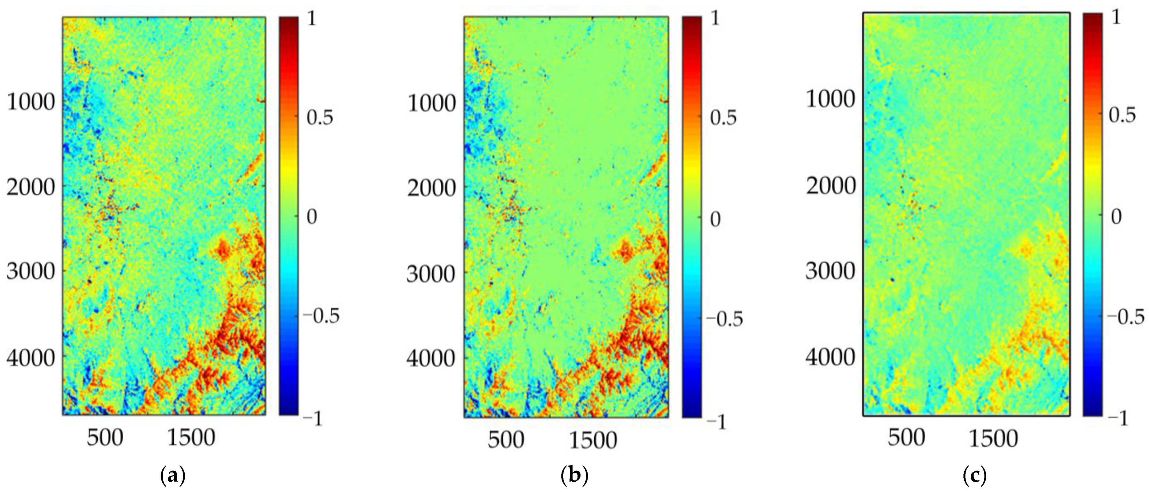
The orbital phase error is manifested in the SAR coordinate system, rendering data fusion unfeasible at this stage. Therefore, one pair of TDX/TSX data was selected for analyzing the model’s correction effect. The results are depicted in Figure 3. It was observed that the orbital phase error was uniformly distributed across the entire study area, manifesting as a large light-yellow hue in Figure 3a. After applying the correction using Equation (4), the majority of the light-yellow hue in Figure 3b is eliminated due to the removal of orbital phase errors, indicating that the model is capable of effectively removing such errors (see a difference in Figure 3c).
Terrain-related phase error is induced by intricate terrain features within the region. Due to the short wavelength of the X-band, areas with significant terrain fluctuations exhibit more dense stripes on the interferogram, which can impede phase unwrapping and even result in failure. To mitigate the impact of terrain on unwrapping, an external DEM is commonly employed, and a differential phase unwrapping technique is utilized to recover residual terrain information [32]. The atmospheric phase error is caused by factors such as signal delay or the tilted propagation path of radar signals affected by the atmosphere during propagation. However, due to the unique imaging conditions of the TDX bistatic mode, the effects of atmospheric disturbances and temporal decoherence can be effectively mitigated [33]. The slant distance measurement error primarily arises from the bias measurement timing system. However, the TDX’s positioning accuracy for slant distance can be controlled within 30 cm, which is nearly an order of magnitude higher than its nominal accuracy (2 m). As a result, the impact of the slant distance measurement error on DEM accuracy may be disregarded [34].
After correcting for the orbital and terrain phase errors that affect phase unwrapping in TanDEM-X DEM, it was determined that the systematic error is primarily influenced by terrain features such as slope, aspect, and elevation. To investigate the relationship between the elevation and TanDEM-X DEM error, we divided the error into four groups based on elevation values: 300–500 m, 500–700 m, 700–900 m, and >1100 m. As depicted in Figure 4a, a positive correlation exists between the error of TanDEM-X DEM and elevation. As illustrated in Figure 4b, there is a quadratic functional relationship between DEM error and terrain slope. As demonstrated in Figure 4c, no significant linear trend can be observed between the TanDEM-X DEM error and terrain aspect.
After conducting the aforementioned analysis, it was determined that the systematic errors in TanDEM-X DEM are primarily associated with elevation and terrain slope. Consequently, a polynomial model for TanDEM-X DEM is expressed as follows:
h = a 0 + a 1 x + a 2 y + a 3 x 2 + a 4 x y + a 5 y 2 + a 6 h + a 7 s + a 8 s 2
where h represents the difference in elevation between the ICESat-2 data and TanDEM-X DEM, x and y denote the longitude and latitude coordinates, h denotes the elevation of ICESat-2 data, s indicates its slope, and a i ( i = 0 , 1 , , 8 ) are unknown coefficients to be determined.

3.3. LSC-TXC Algorithm for TanDEM-X DEM Error Correction

3.3.1. Observation Equation System

The LSC method was originally developed by Moritz (1972) [35] and has become a well-known algorithm for filtering and predicting geodetic and geophysical observations simultaneously, including trend signal errors and noises [36,37]. The core idea of the LSC method is that trend signal errors and noises are first incorporated into the same equation system. Then, solutions of the concerned unknown parameters in the same equation system are solved with the assistance of sparse high-precision observations. The equation system can be expressed as:
L = B X + G Y +
where L represents observation vector, B represents the coefficient matrix; X = X   X T is the focused unknown parameters part of the model, where X and X represent the focused unknown parameters where auxiliary high-precision observations are available (referred to as the coincidence point) and unavailable (referred to as the non-coincidence point), respectively. G Y represents the contribution of trend signal components on the observation vector L, where G is the coefficient matrix of the contribution of systematic error parameters Y . is white noise of the observations.
According to the analysis in Section 3.2, the systematic errors of TanDEM-X DEM are spatially correlated with pixel locations (x, y), elevations, and slopes. Therefore, we used a polynomial relating to the correlation factors to describe the systematic error pattern of TanDEM-X DEM; that is, the second term in the right side of Equation (6) can be expressed as:
G = 1 x 1 y 1 x 1 2 x 1 y 1 y 1 2 h 1 s 1 s 1 2 1 x 2 y 2 x 2 2 x 2 y 2 y 2 2 h 2 s 2 s 2 2 1 x m y m x m 2 x m y m y m 2 h m s m s m 2
Y = a 0    a 1    a 2    a 3    a 4    a 5    a 6    a 7    a 8 T
where a 0 to a 8 in Y denote the systematic parameters which are unknown and need to be solved. The main reason for utilizing the LSC method is to obtain more accurate elevations by mitigating systematic and random errors from TanDEM-X DEM. Therefore, the matrix X in Equation (6) is a vector consisting of unknown elevations in the region of interest. The coefficient matrix B is an identity matrix. The observation vector is composed of auxiliary high-accuracy observations obtained by ICESAT-2, GEDI, GNSS, and so on.

3.3.2. Error Correction of TanDEM-X DEM

Having obtained the equation system relating systematic and random errors to elevation observations, the solutions for the elevations after systematic and random error mitigation can be found. According to Moritz (1972) [35], the error equation systems of Equation (6) can be expressed as follows:
V = B X ^ + G Y ^ L V X = X ^ L X V X = X ^ L X
where the caret denotes the solutions of X and Y, and V denotes the residual vector. Considering that noises are independent of X and X , the variances between them are zeros, i.e., D X = 0 and D X = 0 . The solutions of the unknown parameter of Equation (8) can be estimated with Equation (10) based on the minimization of the mean squared error of observations and the focused unknown parameters, as follows:
Y ^ = G T B D X B T + D 1 G 1 G T B D X B T + D 1 L B L X X ^ = L X + D X B T B D X B T + D 1 ( L G Y ^ B L X ) X ^ = L X + D X X B T B D X B T + D 1 ( L G Y ^ B L X )
where D X and D are the variances of X and , respectively, and D X X denotes the covariance of the elevations where auxiliary observations are available and unavailable.
Following the matrix transformation, Equation (10) can be simplified as follows:
Y ^ = G T D X X 1 G 1 G T D X X 1 L X ^ = D X X D X X 1 ( L G Y ^ ) X ^ = D X X D X X 1 ( L G Y ^ )
where D X X is the self-covariance matrix of elevations where auxiliary observations are available; D X X is the covariance matrix of elevations where auxiliary observations are unavailable and available.
As observed in Equation (11), the key to estimate the elevations after systematic and random error mitigation is to determine the matrices D X X and D X X in Equation (11) [38]. In this study, the prior covariance of trend systematic errors (namely Cr) between two points, i and j , within a distance threshold of r is given by:
C r = 1 N r P i P j
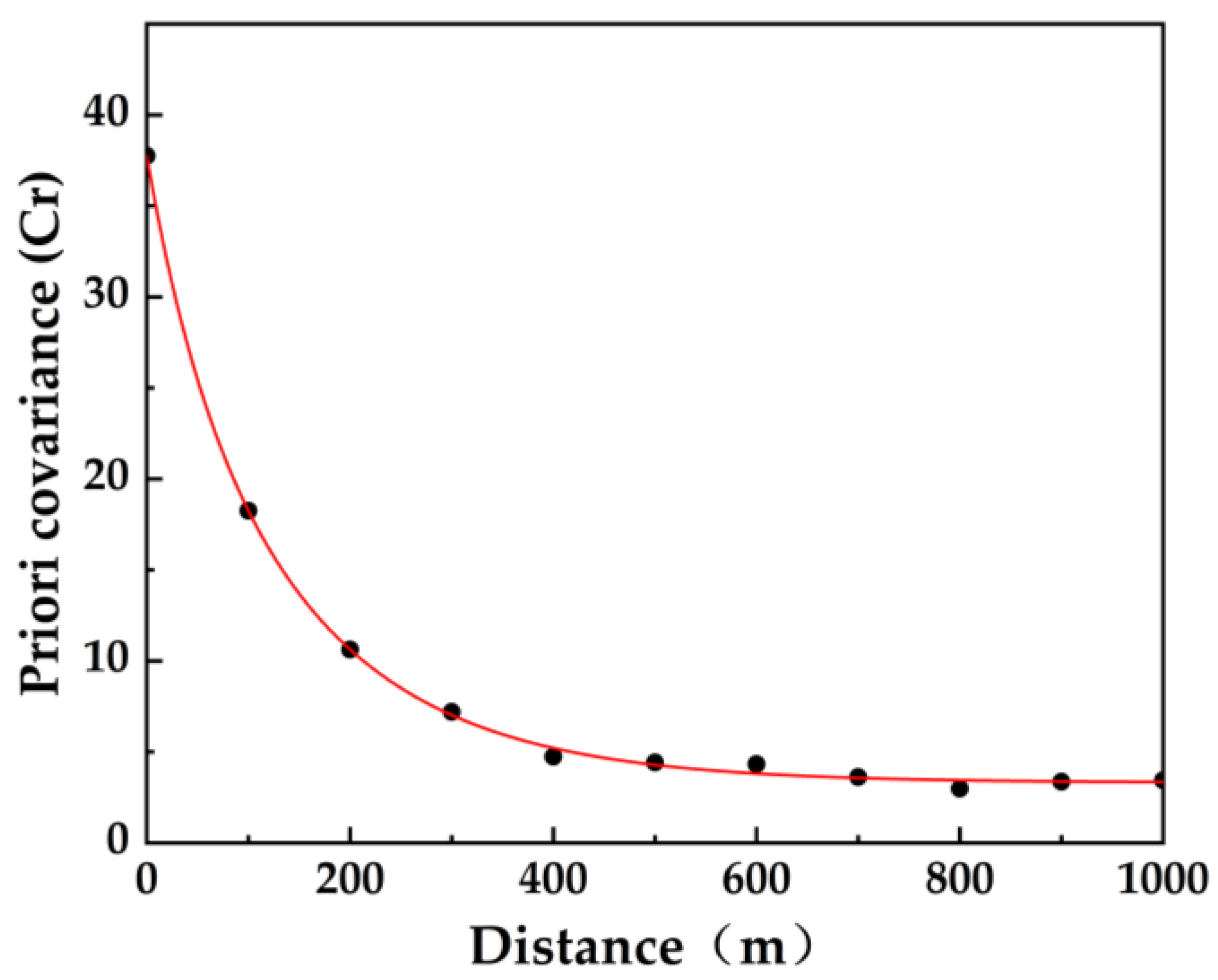
where N r is the total number of paired coincident points spaced apart by a distance r , and P i P j is the product of the signals. Once auxiliary high-precision observations with acceptable density are available, the covariance matrix can be obtained by fitting. The interval distance r has an impact on both the prior covariance calculation and covariance function fitting. In this paper, we adopt Wojciech’s method [39] for determining the optimal spacing distance r by calculating the relationship between an a priori covariance value of the coincident points and the spacing distance, as shown in Figure 5. The stability of the a priori covariance value tends to occur at interval distances greater than 400 m, beyond which they remain essentially unchanged. Therefore, by selecting r = 400 m as the optimal spacing distance in the region, we can calculate an a priori covariance value that meets our requirements.
According to the above process, the distance and prior covariance between each pair of coincidence points can be obtained, and then the optimal curve function is estimated by using the least-square fitting to describe the relationship between the distance of each pair of coincidence points and its prior covariance. Afterwards, the variance–covariance matrix (VCM) is generated for the two signals between the coincident and non-coincident points based on the obtained optimal-fit curve or covariance function. The VCM can be expressed as follows:
D X X D X X D X X T D X X
where D X X is the autocovariance matrix of the non-coincidence points, D X X denotes the cross-covariance matrix between coincident and non-coincident points, while D X X signifies the autocovariance matrix of the coincidence points.
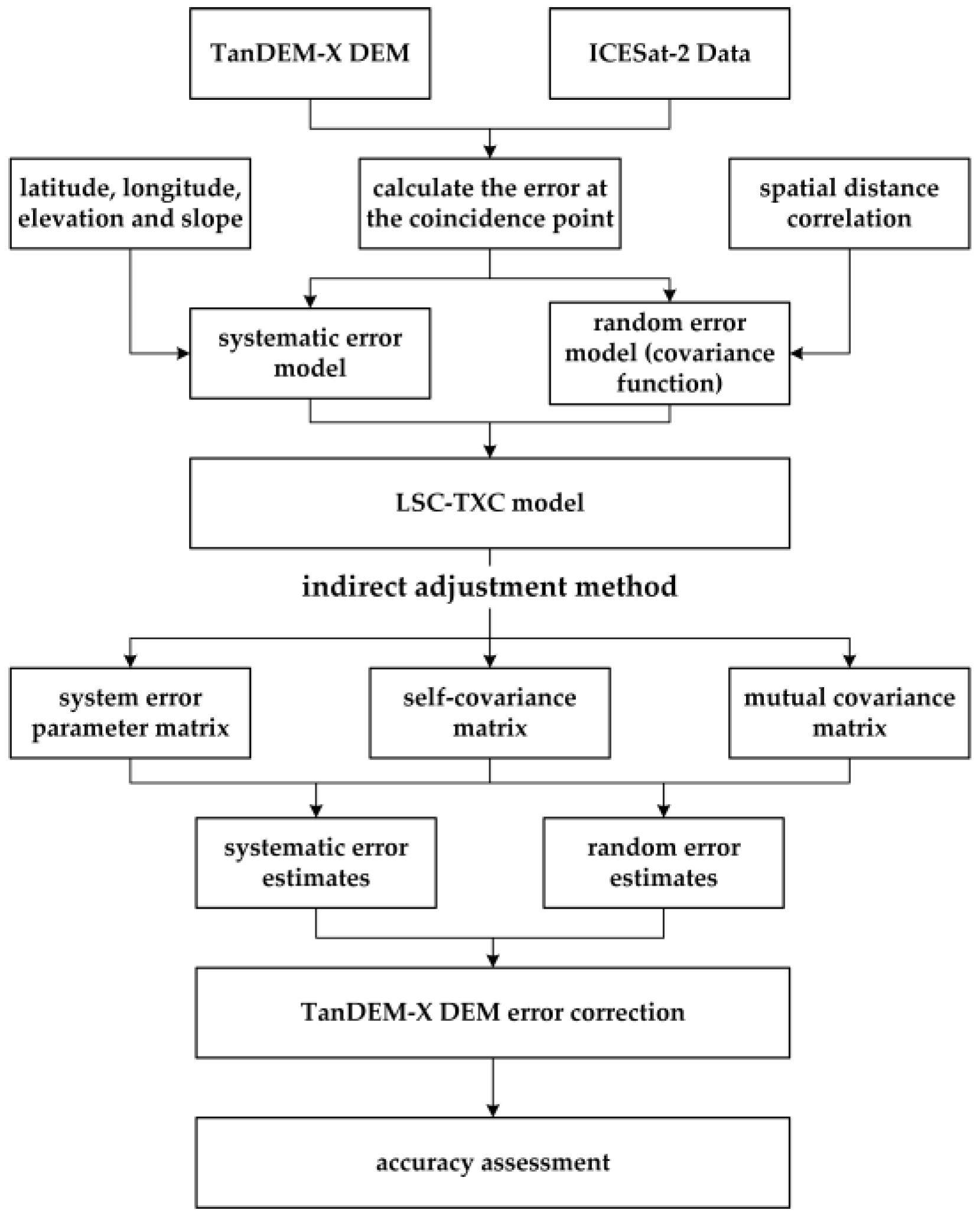
Finally, D X X and D X X are substituted into Equation (11), and the estimates Y ^ ,    X ^ and X ^ can be obtained. The errors for all raster points of the TanDEM-X DEM can be calculated by substituting the obtained estimates into Equation (6). The corrected DEM can be generated by subtracting these errors from the original TanDEM-X DEM. The specific workflow of the LSC-TXC algorithm presented in this paper is shown in Figure 6.

4. Results

4.1. TanDEM-X DEM Correction Results

This study utilizes 23,250 ICESat-2 altimetry data points acquired in 2021 within the designated study area as experimental data, followed by a random selection of 12,036 ICESat-2 data points within the same area in 2022 for validation purposes. The validation dataset is employed to assess the accuracy variations of TanDEM-X DEM pre-correction and post-correction. The primary evaluation metrics comprise the mean error (ME) and root mean square error (RMSE). The corresponding calculation formulas for these two metrics are as follows:
M E = 1 n i = 1 n x i y i
R M S E = i = 1 n x i y i 2 n
where n represents the number of validation data points, x denotes the elevation value of each validation point, and y represents the corresponding elevation value in the DEM. The unit for elevation data is meters.
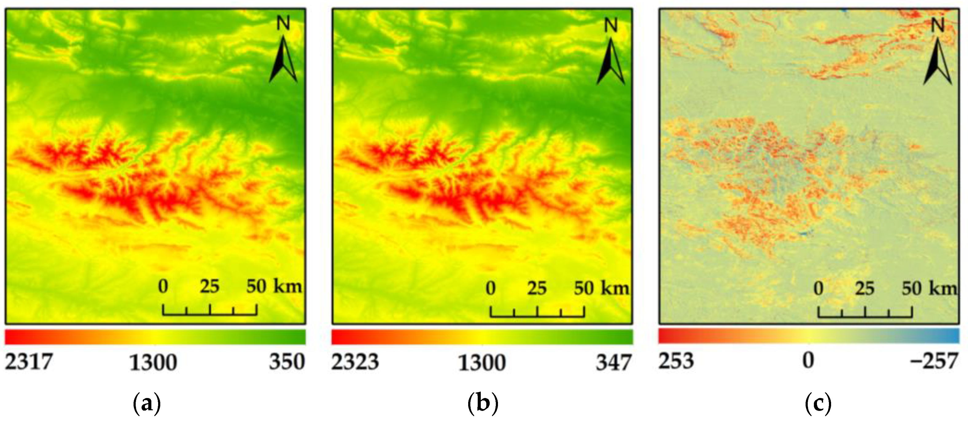
Figure 7a displays the original TanDEM-X DEM, and Figure 7b exhibits the TanDEM-X DEM corrected by the LSC-TXC algorithm presented in this paper. While Figure 7c illustrates the elevation difference between the corrected TanDEM-X DEM and the original TanDEM-X DEM. The findings indicate that the differences are pre-dominantly concentrated within the range of −20 m to 30 m, which is consistent with the outcomes of the TanDEM-X DEM accuracy assessment [40]. However, the largest difference between the grids is −257.255 m, and there are dozens of grids with differences of more than 100 m. After analysis, we found that the original TanDEM-X DEM had data gaps in these regions, which were filled by LSC-TXC algorithm, resulting in abnormal height difference in these grid regions.
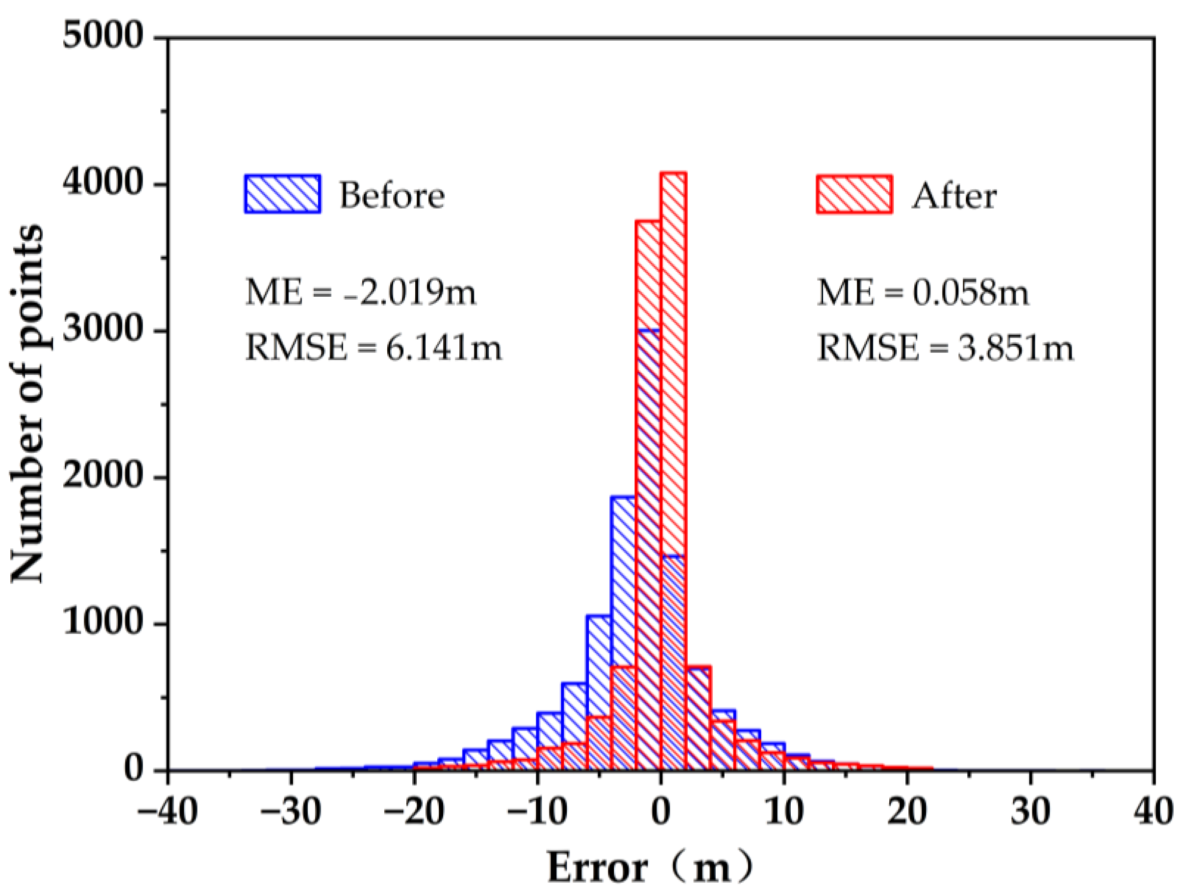
The difference between the ICESat-2 validation data and corresponding point elevations of TanDEM-X DEM before and after the correction can be calculated, yielding an error histogram as depicted in Figure 8. Prior to the correction, TanDEM-X DEM exhibited a degree of negative deviation with a ME of −2.019 m, indicating that its elevation was on average higher than that of the ICESat-2 points. The observed situation is attributed to the location of the TanDEM-X radar satellite’s observation center, which lies between the vegetation canopy and exposed surface. The pre-correction RMSE stands at 6.141 m, a figure that aligns with those found in other regions. For instance, Gdulová K et al. [40] reported an RMSE of 11.99 m for TanDEM-X DEM in certain European mountainous areas while Yu et al. [41] discovered an RMSE of 7.87 m for TanDEM-X DEM in China.
After the correction, the vertical error in TanDEM-X DEM is symmetrically distributed around zero. Compared to before correction, the vertical error in TanDEM-X DEM is closer to zero with an ME of 0.058 m. After the correction, Figure 8 demonstrates a significant reduction in the number of points with larger error values and a decrease in RMSE to 3.851 m. These results indicate that the algorithm proposed in this paper effectively enhances the quality of TanDEM-X DEM.
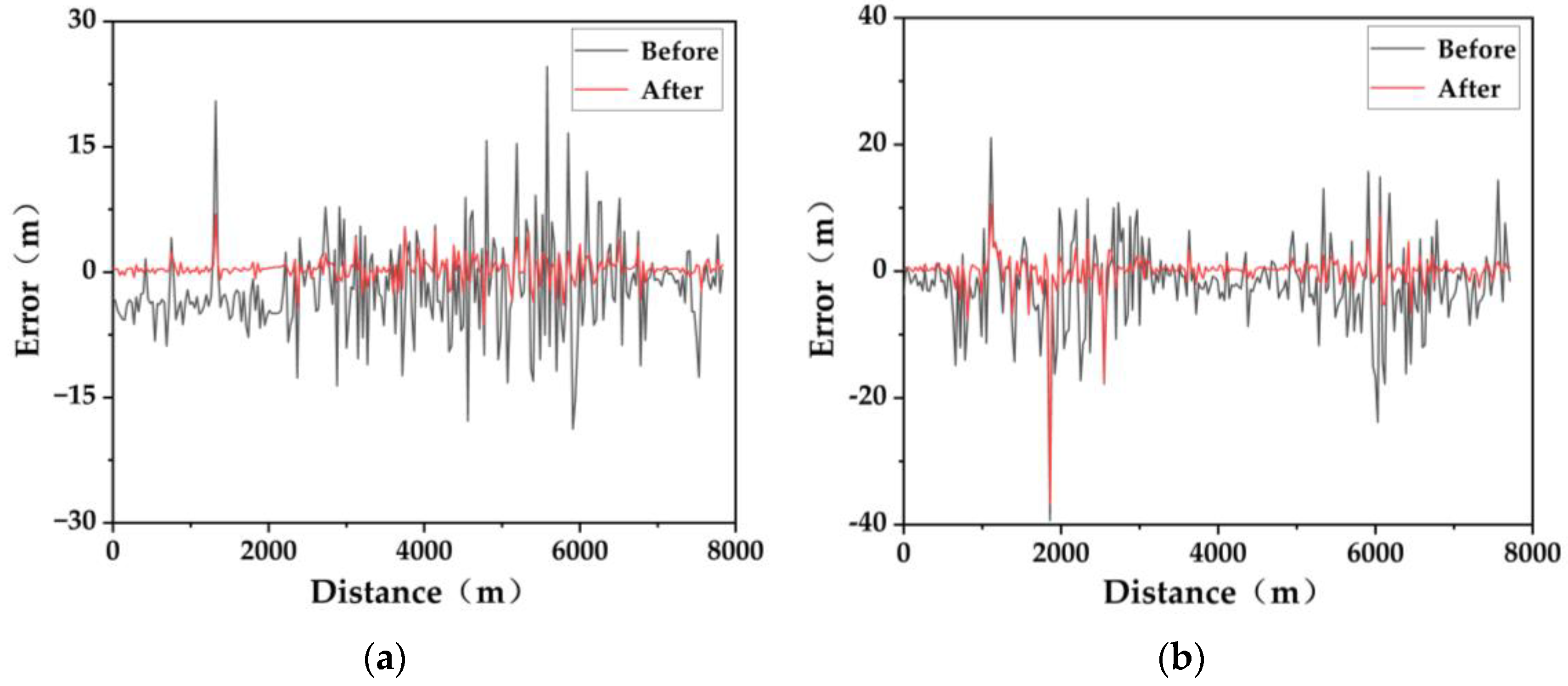
To validate the efficiency of the presented algorithm in rectifying systematic and random errors in TanDEM-X DEM, two profile lines exhibiting significant terrain variations within the study area were selected to demonstrate local error changes before and after the correction. The error trend line after the correction in Figure 9b is smoother and closer to zero, corresponding to Figure 9a, indicating that the LSC-TXC algorithm effectively mitigates systematic errors in TanDEM-X DEM. Meanwhile, the errors that suddenly change before the correction (these are random errors) are well corrected by the presented algorithm, indicating that the LSC-TXC algorithm effectively corrects random errors in TanDEM-X DEM. However, the correction effect of random errors is not statistically significant in the vicinity of 2000 m along the profile line as shown in Figure 9b. This can be attributed to insufficient ICESat-2 experimental data points within this range, leading to inadequate coincidence points for calculating the spatial correlation between signals.

4.2. Influence of Terrain Factors on TanDEM-X DEM Correction Results

This study integrates corresponding terrain slope data to construct a plot illustrating the relationship between the TanDEM-X DEM error and terrain slope, both before and after correction. As depicted in Figure 10a, prior to the correction, the error value of TanDEM-X DEM gradually increases with increasing slope, indicating a trend of gradual divergence on the scatter plot. The relationship depicted in Figure 10b appears to vanish upon the implementation of the accuracy enhancement algorithm. Following the correction, the gradual increase trend of TanDEM-X DEM error value with slope augmentation is no longer discernible, and scatter plot divergence is no longer evident. The fitting curve remains relatively stable at the zero level, indicating that the algorithm presented in this article effectively mitigates terrain slope-induced DEM errors.
Then, the terrain slope, undulation, and elevation of the study area are categorized into different levels. Grade I encompasses a terrain slope ranging from 0–5°, surface relief between 0 and 30 m, and an elevation of 300–700 m. Grade II terrain includes terrain slopes of 5–10°, surface relief ranging from 30–60 m and elevations between 700–1300 m. Grade III terrain is characterized by slopes of 10–15°, surface relief ranging from 60–90 m and elevations between 1300–1700 m. Grade IV pertains to terrain with a slope ranging from 15–20°, surface relief measuring between 90–120 m, and elevations between 1700–2100 m. Grade V encompasses terrain with a slope greater than 20°, surface undulation exceeding 120 m and an elevation surpassing 2100 m.
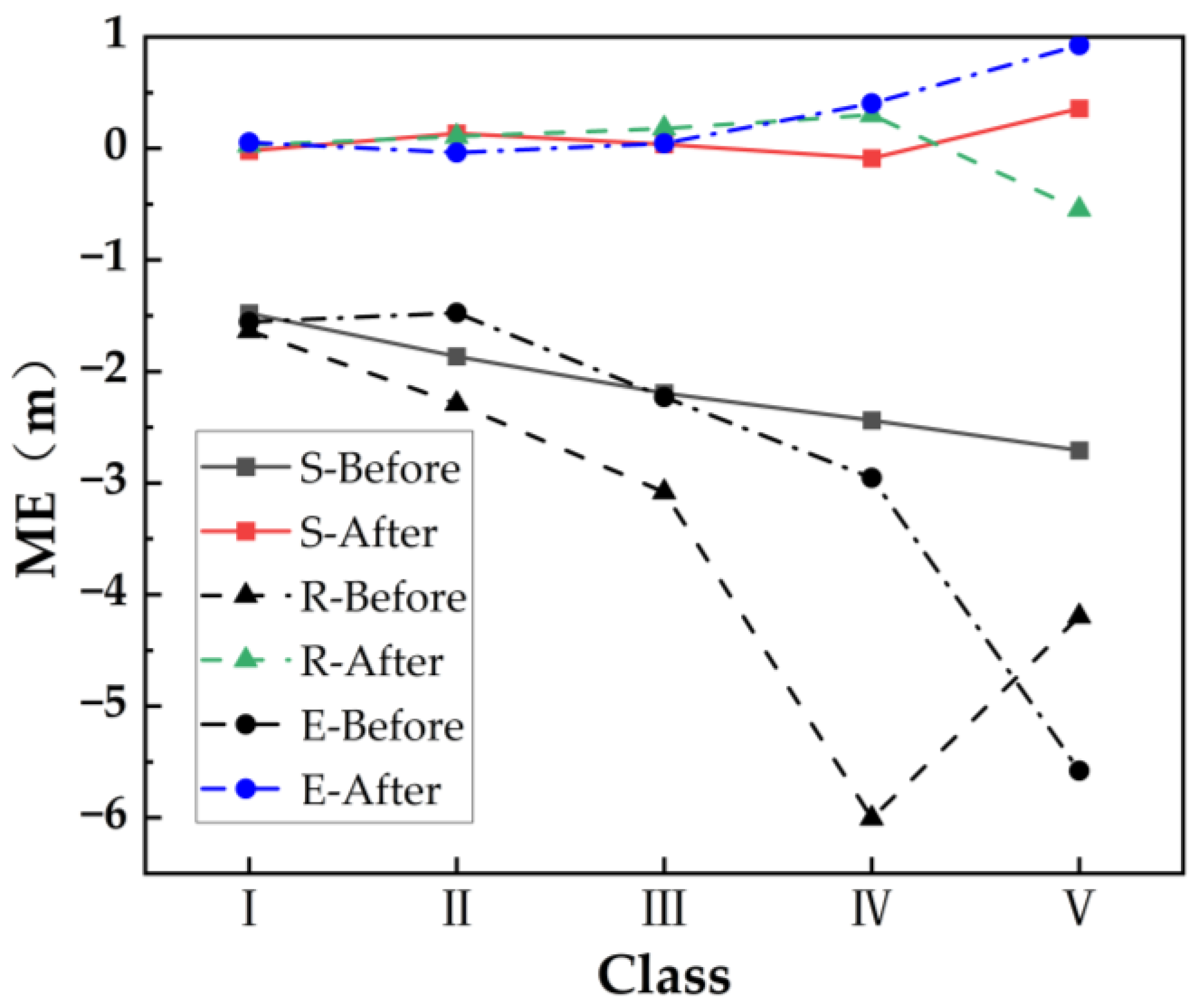
Table 1 and Figure 11 demonstrate the impact of terrain slope, relief, and elevation grade on the ME of TanDEM-X DEM (pre- and post-correction). It is evident that prior to the correction, the ME exhibits an increasing trend with respect to improvements in these three terrain factors. The primary cause of non-conforming situations at grade II and IV is attributed to significant random errors occurring at these levels. After the correction, it is evident that the algorithm proposed in this paper exhibits a significant improvement in the error of previous terrain factor grades (I, II and III), with an improved ME approaching zero. The enhancement effect of ME for grades IV and V is slightly suboptimal, primarily due to the intricate topography in high terrain factor regions, leading to a lower accuracy of ICESat-2 measurements compared to flat terrain areas.
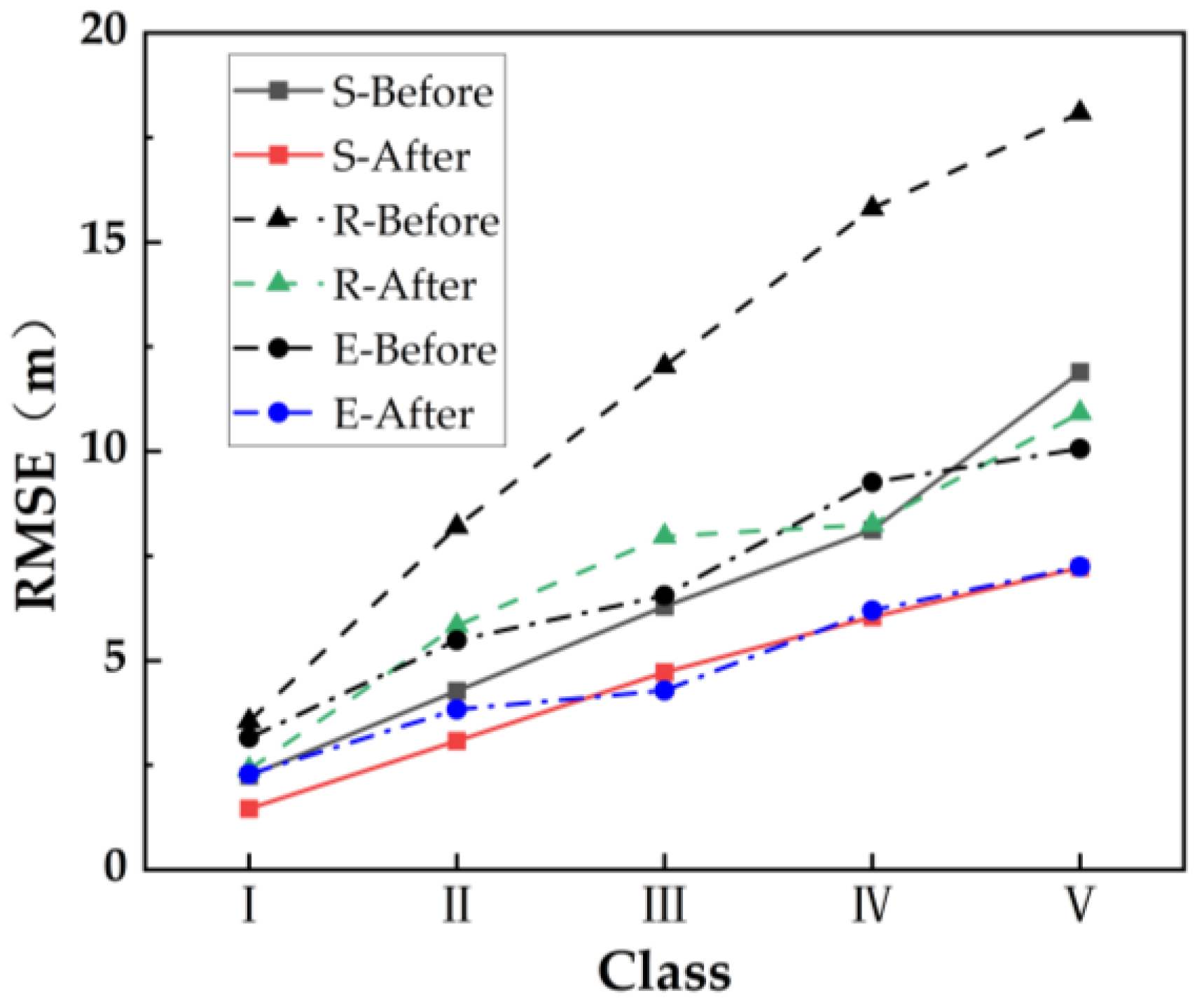
Table 1 and Figure 12 demonstrate the impact of terrain slope, relief, and elevation grade on the RMSE of TanDEM-X DEM (pre- and post-correction). It is evident that a strong positive correlation exists between topographic factors and the RMSE of TanDEM-X DEM both before and after the correction. After the correction, the RMSE of TanDEM-X DEM is consistently lower than its uncorrected counterpart across all terrain factor grades. Notably, the highest accuracy correction effect is observed at grade V.

4.3. Influence of Land Use on TanDEM-X DEM Correction Results

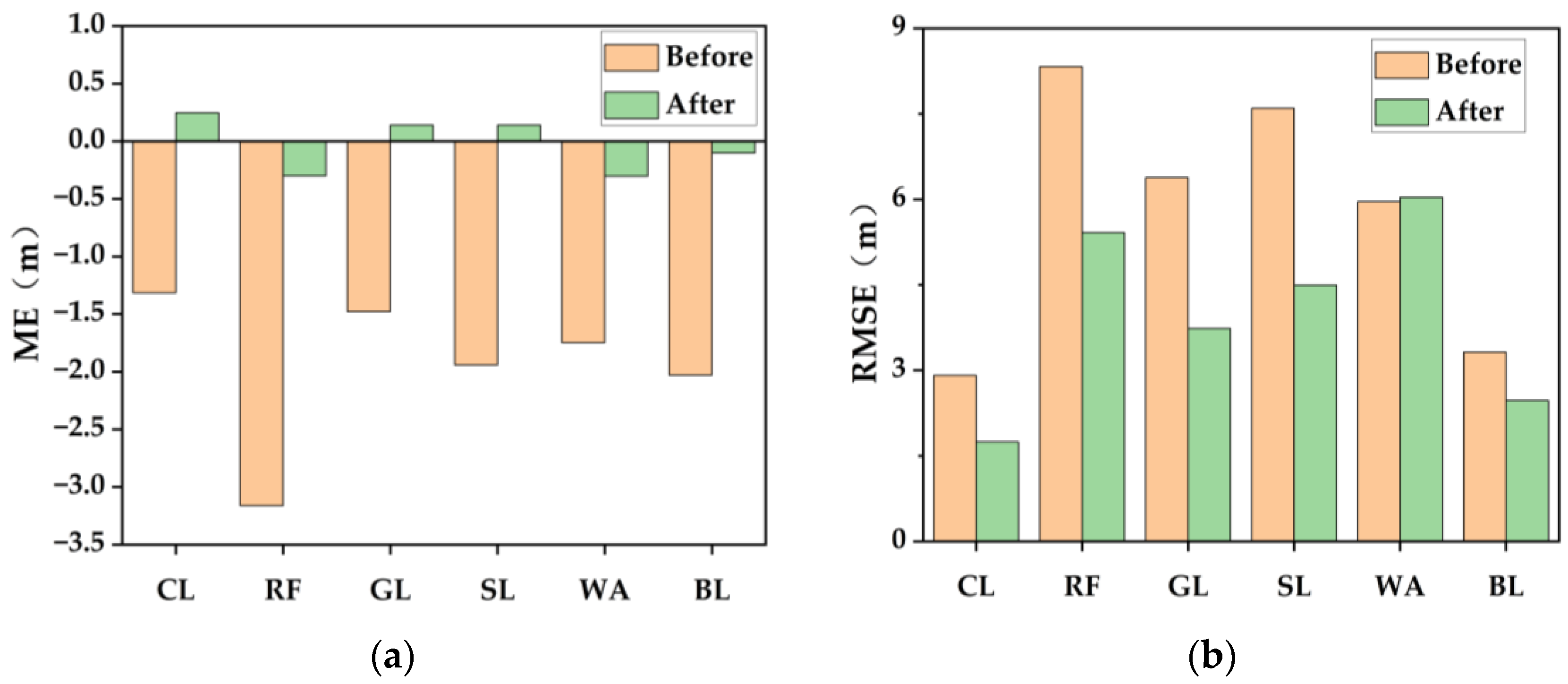
This paper integrates corresponding land use type data to illustrate the relationship between TanDEM-X DEM’s ME and RMSE with respect to land use types. As depicted in Figure 13, land use types significantly affect the ME and RMSE of TanDEM-X DEM. Prior to the correction, forest areas exhibit the largest absolute value of ME (2.559 m), while water areas have the smallest (1.256 m). The forest area exhibits the largest RMSE (7.718 m), while the cultivated area displays the smallest (2.860 m). Amongst all six land use types, the absolute values of ME and RMSE are highest in forest areas due to the irregular backscattering of SAR radar signals caused by tree trunks and branches, leading to amplified geometric distortion. After the correction, it can be observed that the accuracy of other land use categories has significantly improved, except for water areas. The RMSE for water areas has increased post-correction (i.e., decreased accuracy), which is attributed to low error correlation in these regions and persistent gaps in TanDEM-X DEM coverage.

4.4. Model Performance Comparison

Table 2 shows the performance comparison between the LSC-TXC algorithm proposed in this paper and various other models for DEM correction.
It can be found that the ME and RMSE of TanDEM-X DEM corrected by LSC-TXC, Random Forest (RF) [42], Height Difference Fitting Neural Network (HDFNN) [43], and Back Propagation Neural Network (BPNN) [44] are reduced compared to the TanDEM-X DEM (ME = −2.019 m, RMSE = 6.141 m), indicating that the four correction models have effectively enhanced the accuracy of the original TanDEM-X DEM in this study area. The ME of the RF (−0.033 m) outperforms that of the LSC-TXC algorithm proposed in this paper (0.058 m).
The LSC-TXC algorithm proposed in this paper exhibits a significantly superior performance in correcting TanDEM-X DEM, as compared to the other three algorithms with respect to RMSE. Specifically, the accuracy of TanDEM-X DEM corrected by the LSC-TXC algorithm has been observed to improve by 6.5%, 7.6%, and 18.1% when compared against RF, HDFNN, and BPNN, respectively. For these three algorithms, RF has the best performance due to its adoption of bootstrap aggregation scheme in regression, which collects data from all samples for model training, and uses other data for verification. This strategy effectively avoids overfitting problems commonly encountered by linear regression methods in classical machine learning [45]. However, since RF involves four stages that are time consuming, the computational cost of this model is relatively high.

5. Discussion

In the process of error correction for TanDEM-X DEM using the LSC-TXC algorithm proposed in this paper, we found that the error estimate at a non-coincident point is determined by fitting the covariance value calculated between that non-coincident point and all coincident points within a certain range. Therefore, the selection of spatial distance will inevitably impact the correction results of TanDEM-X DEM. Moreover, we obtained the optimal spacing distance (400 m) in the region by fitting the relationship between priori covariance and spacing distances for each coincident point during an a priori covariance calculation in Section 4.2. To determine the optimal spacing distance for this study, we conducted a calculation of the RMSE of TanDEM-X DEM correction at various spatial intervals, as presented in Table 3.
As can be seen from Table 3, the LSC-TXC algorithm presents distinct error corrections for spatially correlated errors at different spatial distances. The optimal spatial distance for the correction is found to be 400 m, where the minimum RMSE is observed. However, when the selected spatial distance exceeds 400 m, the RMSE gradually increases again until it reaches its maximum at a spatial distance of 200 m. It is shown that the errors at the coincident and non-coincident points have a strong spatial correlation when the spatial distance is set to 400 m in this study, which makes the LSC-TXC algorithm optimal for correcting errors within this range. Therefore, if the selection spatial distance is too small, the number of coincident points involved in the calculation may be insufficient or it may fail to cover the whole study area, resulting in correction results. If the selected spatial distance is excessively large, the correction results will be affected by the weak correlation between non-coincident points and coincident points that are too distant.
Whether the systematic error model developed in this paper can accurately describe the true systematic error is somewhat dependent on the size of the region involved in the error analysis, while the correlation of the systematic errors is related to their distance from each other at each point. Generally speaking, the larger the area covered by the systematic error model, the more challenging it becomes for the model to accurately describe the true systematic error. Meanwhile, as points become further apart from each other, their correlation weakens. Therefore, the subsequent research direction will focus on exploring the optimal region size for the systematic error model and selecting the most appropriate distance between systematic errors to calculate the spatial correlation. Further experimental results are required to verify these.

6. Conclusions

The aim of this study was to improve the elevation accuracy of TanDEM-X DEM, expand its application scope and application potential. In this paper, a region with rich topographic features in southwest Europe is selected as the research area. An error correction algorithm for TanDEM-X DEM based on least-square collocation (LSC-TXC) is proposed. This algorithm not only eliminates the systematic errors of a wide range of trends, but also eliminates random errors well. Experimental results show that the RMSE of TanDEM-X DEM corrected by the LSC-TXC algorithm was reduced from 6.141 m to 3.851 m, with a 37.3% improvement in accuracy. Meanwhile, the LSC-TXC algorithm effectively mitigates DEM errors induced by elevation, topographic slope and surface relief, exhibiting a favorable correction performance across various land use types. Compared to three conventional algorithms, namely Random Forest, Height Difference Fitting Neural Network, and Back Propagation in Neural Network, the presented algorithm demonstrates a reduction in TanDEM-X DEM’s RMSEs by 6.5%, 7.6%, and 18.1%, respectively. This algorithm provides an efficient tool for correcting DEMs such as TanDEM-X for a wide range of areas.

Author Contributions

Conceptualization, X.S., C.Z. and J.Z.; methodology, X.S.; software, X.S.; validation, X.S. and C.Z.; formal analysis, X.S. and C.Z.; investigation, X.S.; resources, C.Z.; data curation, C.Z.; writing—original draft preparation, X.S.; writing—review and editing, X.S. and C.Z.; visualization, X.S.; supervision, C.Z. and J.Z.; project administration, C.Z.; funding acquisition, C.Z. and J.Z. All authors have read and agreed to the published version of the manuscript.

Funding

This research was funded by the National Natural Science Foundation of China (No. 42074016 and 42030112).

Data Availability Statement

Not applicable.

Acknowledgments

Many thanks to NASA, USGS for providing free datasets. The authors would like to thank Zefa Yang and Tao Zhang from the Central South University, for the helpful discussions on the least-squares collocation-based error correction method.

Conflicts of Interest

The authors declare no conflict of interest.

References

  1. Tang, G. Research progress of digital elevation model and digital terrain analysis in China. Acta Geogr. Sin. 2014, 69, 1305–1325. [Google Scholar]
  2. Zhou, C.; Zhang, G.; Yang, Z.; Ao, M.; Liu, Z.; Zhu, J. An adaptive terrain-dependent method for SRTM DEM correction over mountainous areas. IEEE Access 2020, 8, 130878–130887. [Google Scholar] [CrossRef]
  3. Lee, H.; Hahn, M. KOMPSAT-3 digital elevation model correction based on point-to-surface matching. Remote Sens. 2019, 11, 2340. [Google Scholar] [CrossRef] [Green Version]
  4. Li, X.; Shen, H.; Feng, R.; Li, J.; Zhang, L. DEM generation from contours and a low-resolution DEM. ISPRS J. Photogramm. Remote Sens. 2017, 134, 135–147. [Google Scholar] [CrossRef]
  5. Fujita, K.; Suzuki, R.; Nuimura, T.; Sakai, A. Performance of ASTER and SRTM DEMs, and their potential for assessing glacial lakes in the Lunana region, Bhutan Himalaya. J. Glaciol. 2008, 54, 220–228. [Google Scholar] [CrossRef] [Green Version]
  6. Tadono, T.; Takaku, J.; Tsutsui, K.; Oda, F.; Nagai, H. Status of “ALOS World 3D (AW3D)” global DSM generation. In Proceedings of the 2015 IEEE International Geoscience and Remote Sensing Symposium (IGARSS), Milan, Italy, 26–31 July 2015; pp. 3822–3825. [Google Scholar]
  7. Zhao, S.; Liu, J.; Cheng, W.; Zhou, C. Fusion Scheme and Implementation Based on SRTM1, ASTER GDEM V3, and AW3D30. ISPRS Int. J. Geo-Inf. 2022, 11, 207. [Google Scholar] [CrossRef]
  8. Rizzoli, P.; Martone, M.; Gonzalez, C.; Wecklich, C.; Tridon, D.B.; Bräutigam, B.; Bachmann, M.; Schulze, D.; Fritz, T.; Huber, M.; et al. Generation and performance assessment of the global TanDEM-X digital elevation model. ISPRS J. Photogramm. Remote Sens. 2017, 132, 119–139. [Google Scholar] [CrossRef] [Green Version]
  9. Chen, N. Influence of Resolutions of DEM on the Error of Slope. Geomat. Inf. Sci. Wuhan Univ. 2013, 38, 594–598. [Google Scholar]
  10. Florinsky, I.V.; Skrypitsyna, T.N.; Luschikova, O.S. Comparative accuracy of the AW3D30 DSM, ASTER GDEM, and SRTM1 DEM: A case study on the Zaoksky testing ground, Central European Russia. Remote Sens. Lett. 2018, 9, 706–714. [Google Scholar] [CrossRef]
  11. Girohi, P.; Bhardwaj, A. InSAR-Based Digital Elevation Model (DEM) Improvement Using Data Fusion Technique with Neural Networks on Diverse Topographic Indian Regions. Authorea Prepr. 2022, 4, 625–646. [Google Scholar]
  12. Girohi, P.; Bhardwaj, A. A Neural Network-Based Fusion Approach for Improvement of SAR Interferometry-Based Digital Elevation Models in Plain and Hilly Regions of India. AI 2022, 3, 820–843. [Google Scholar] [CrossRef]
  13. Qin, X.; Zhang, H.; Heng, Z.; Yu, W.; Huayou, L. A High Precision DEM Generation Method Based on Ascending and Descending Pass TerraSAR-X/TanDEM-X BiSAR Data. J. Radars 2018, 7, 487–497. [Google Scholar]
  14. Podgórski, J.; Kinnard, C.; Pętlicki, M.; Urrutia, R. Performance Assessment of TanDEM-X DEM for Mountain Glacier Elevation Change Detection. Remote Sens. 2019, 11, 187. [Google Scholar] [CrossRef] [Green Version]
  15. Ke, L.; Song, C.; Yong, B.; Lei, Y.; Ding, X. Which heterogeneous glacier melting patterns can be robustly observed from space? A multi-scale assessment in southeastern Tibetan Plateau. Remote Sens. Environ. 2020, 242, 111777. [Google Scholar] [CrossRef]
  16. Wu, Q.; Song, C.; Liu, K.; Ke, L. Integration of TanDEM-X and SRTM DEMs and spectral imagery to improve the large-scale detection of opencast mining areas. Remote Sens. 2020, 12, 1451. [Google Scholar] [CrossRef]
  17. Vanthof, V.; Kelly, R. Water storage estimation in ungauged small reservoirs with the TanDEM-X DEM and multi-source satellite observations. Remote Sens. Environ. 2019, 235, 111437. [Google Scholar] [CrossRef]
  18. Li, W.; Wang, C.; Zhu, W. Error spatial distribution characteristics of TanDEM-X 90m DEM over China. J. Geo-Inf. Sci. 2020, 22, 2277–2288. [Google Scholar]
  19. Apeh, O.I.; Uzodinma, V.N.; Ebinne, E.S.; Moka, E.C.; Onah, E.U. Accuracy Assessment of Alos W3d30, Aster Gdem and Srtm30 Dem: A Case Study of Nigeria, West Africa. J. Geogr. Inf. Syst. 2019, 11, 111–123. [Google Scholar] [CrossRef] [Green Version]
  20. Kim, D.E.; Liong, S.Y.; Gourbesville, P.; Andres, L.; Liu, J. Simple-yet-effective SRTM DEM improvement scheme for dense urban cities using ANN and remote sensing data: Application to flood modeling. Water 2020, 12, 816. [Google Scholar] [CrossRef] [Green Version]
  21. Elshambaky, H.T. Using direct transformation approach as an alternative technique to fuse global digital elevation models with GPS/levelling measurements in Egypt. J. Appl. Geod. 2019, 13, 159–177. [Google Scholar] [CrossRef]
  22. Yue, G.; Liu, Y.; Zheng, C. Study on DEM Fusion Methods Based on InSAR Technology in Complex Terrain Areas. Geomat. Spat. Inf. Technol. 2021, 44, 205–209+214. [Google Scholar]
  23. Mason, D.C.; Trigg, M.; Garcia-Pintado, J.; Cloke, H.L.; Neal, J.C.; Bates, P.D. Improving the TanDEM-X Digital Elevation Model for flood modelling using flood extents from Synthetic Aperture Radar images. Remote Sens. Environ. 2016, 173, 15–28. [Google Scholar] [CrossRef] [Green Version]
  24. Kim, D.E.; Liu, J.; Liong, S.Y.; Gourbesville, P.; Strunz, G. Satellite DEM improvement using multispectral imagery and an artificial neural network. Water 2021, 13, 1551. [Google Scholar] [CrossRef]
  25. Guo, C.; Nie, J.; Tian, J. Vertical deformation analysis of adaptive fusion of GNSS level elevation change. Geomat. Inf. Sci. Wuhan Univ. 2020, 45, 7–12. [Google Scholar]
  26. Trojanowicz, M.; Osada, E.; Karsznia, K. Precise local quasigeoid modelling using GNSS/levelling height anomalies and gravity data. Surv. Rev. 2020, 52, 76–83. [Google Scholar] [CrossRef]
  27. Lü, J.; Zhang, Z.; Zhang, X.; Liu, Z. Application of combination model of quadric surfaces and least squares collocation in GPS height anomaly fitting. Bull. Surv. Mapp. 2020, 5, 127–129. [Google Scholar]
  28. Rehman, K.; Fareed, N.; Chu, H.-J. NASA ICESat-2: Space-Borne LiDAR for Geological Education and Field Mapping of Aeolian Sand Dune Environments. Remote Sens. 2023, 15, 2882. [Google Scholar] [CrossRef]
  29. Jin, G.; Xu, Q.; Zhang, H. Synthetic Aperture Radar Interferometry; National Defense Industry Press: Beijing, China, 2014. [Google Scholar]
  30. Du, Y.; Fu, H.; Liu, L.; Feng, G.; Peng, X.; Wen, D. Orbit error removal in InSAR/MTInSAR with a patch-based polynomial model. Int. J. Appl. Earth Obs. Geoinf. 2021, 102, 102438. [Google Scholar] [CrossRef]
  31. Zhang, Q.; Zhang, J.; Yue, D. Modern Measurement Data Processing and Application; Surveying and Mapping Press: Beijing, China, 2011. [Google Scholar]
  32. Du, Y.; Feng, G.; Li, Z.; Zhu, J.; Peng, X. Generation of high precision DEM from TerraSAR-X/TanDEM-X. Chin. J. Geophys. 2015, 58, 3089–3102. [Google Scholar]
  33. Gruber, A.; Wessel, B.; Huber, M.; Roth, A. Operational TanDEM-X DEM calibration and first validation results. ISPRS J. Photogramm. Remote Sens. 2012, 73, 39–49. [Google Scholar] [CrossRef]
  34. Zhang, W.; Zhu, W.; Tian, X.; Zhang, Q.; Zhao, C.; Niu, Y.; Wang, C. Improved DEM reconstruction method based on multibaseline InSAR. IEEE Geosci. Remote Sens. Lett. 2021, 19, 4011505. [Google Scholar] [CrossRef]
  35. Helmut, M. Least-squares collocation. Rev. Geophys. 1978, 16, 421–430. [Google Scholar]
  36. Xu, L.; Shao, D.; Wu, X.; Niu, T. Study on deformation and strain characteristics of Yunnan region based on least squares configuration. Sci. Surv. Mapp. 2021, 46, 16–23. [Google Scholar]
  37. Deng, W.; Lan, M.; Wang, H. Dynamic analysis of crust deformation in Xinjiang under least squares configuration. Chin. J. Geol. 2022, 57, 958–974. [Google Scholar]
  38. Ruan, M.; Chen, S.; Han, J. Regional gravity field model constructed by the Least squares collocation. Acta Seismol. Sin. 2020, 42, 53–65. [Google Scholar]
  39. Jarmołowski, W.; Mieczysław, B. Two covariance models in Least Squares Collocation (LSC) tested in interpolation of local topography. Contrib. Geophys. Geod. 2013, 43, 1–19. [Google Scholar] [CrossRef] [Green Version]
  40. Gdulová, K.; Marešová, J.; Moudrý, V. Accuracy assessment of the global TanDEM-X digital elevation model in a mountain environment. Remote Sens. Environ. 2020, 241, 111724. [Google Scholar] [CrossRef]
  41. Yu, J.; Liu, K.; Zhang, B.; Huang, Y.; Fan, C.; Song, C.; Tang, G. Vertical accuracy assessment and applicability analysis of TanDEM-X 90 m DEM in China. J. Geo-Inf. Sci. 2021, 23, 646–657. [Google Scholar]
  42. Chen, C.; Yang, S.; Li, Y. Accuracy assessment and correction of SRTM DEM using ICESat/GLAS data under data coregistration. Remote Sens. 2020, 12, 3435. [Google Scholar] [CrossRef]
  43. Shen, H.; Liu, L.; Yue, L.; Li, X.; Zhang, L. A Multi-source DEM Fusion Method Based on Elevation Difference Fitting Neural Network. Acta Geod. Et Cartogr. Sin. 2018, 47, 854–863. [Google Scholar]
  44. Tang, X.; Feng, D.; Li, K.Q.; Liu, J.; Song, J.; Sheng, V.S. An Improved BPNN Prediction Method Based on Multi-Strategy Sparrow Search Algorithm. Comput. Mater. Contin. 2023, 74, 2789–2802. [Google Scholar] [CrossRef]
  45. Zhao, W.; Wu, H.; Yin, G.; Duan, S.B. Normalization of the temporal effect on the MODIS land surface temperature product using random forest regression. ISPRS J. Photogramm. Remote Sens. 2019, 152, 109–118. [Google Scholar] [CrossRef]
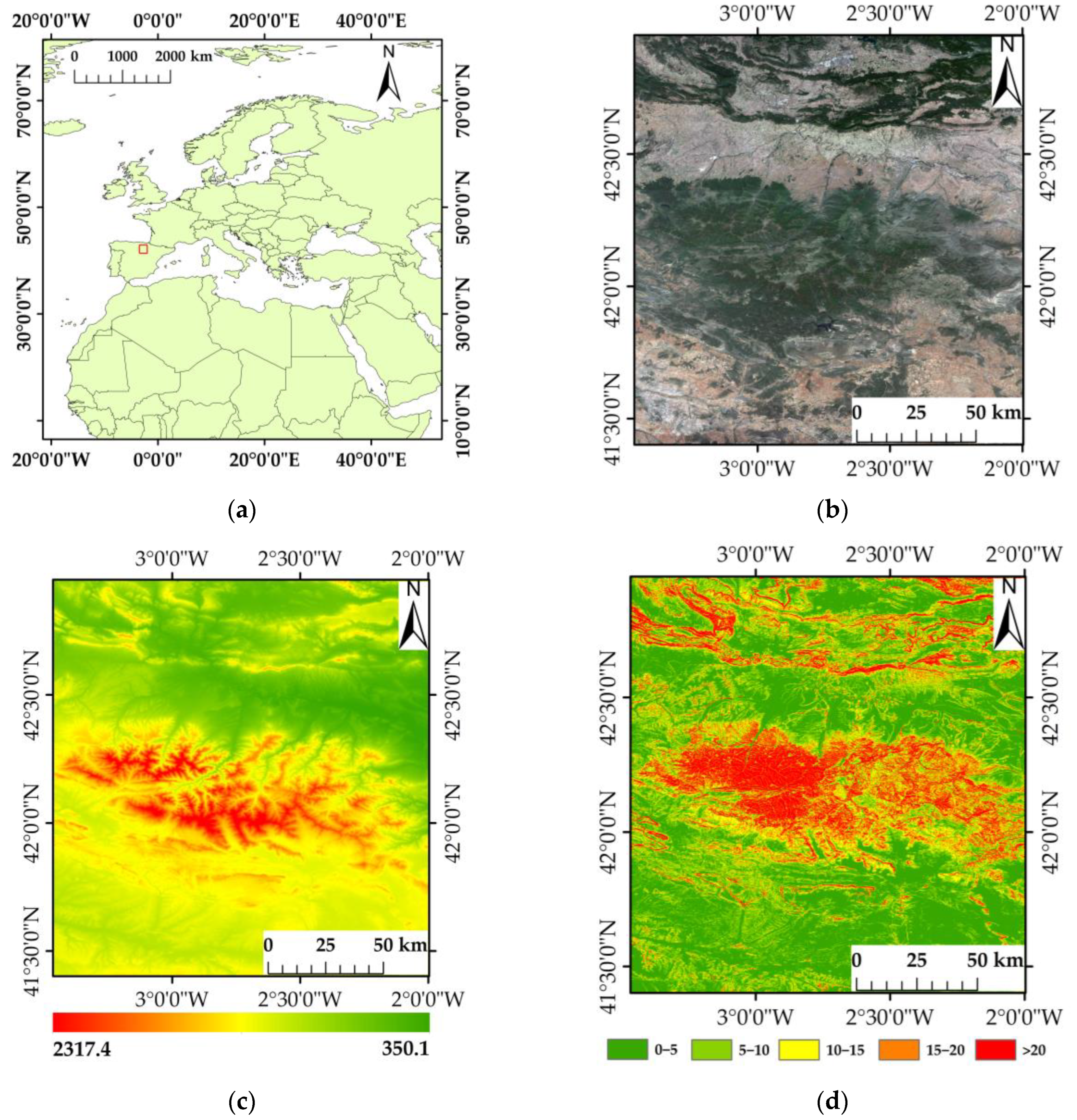
Figure 1. Study site and datasets: (a) location of study area (The red rectangles show the location of the study area), (b) Sentinel-2 satellite image, (c) TanDEM-X DEM, (d) terrain slope.
Remotesensing 15 03695 g001
Figure 2. Schematic diagram of TanDEM-X/TerraSAR-X DEM Generation.
Remotesensing 15 03695 g002
Figure 3. Comparison of the orbital phase error before and after correction, (a) before correction, (b) after correction, (c) Difference Chart.
Remotesensing 15 03695 g003
Figure 4. The relationship between terrain features and TanDEM-X DEM error, (a) elevation error map, (b) terrain slope error map (The red line is the trend line), and (c) terrain slope error map.
Remotesensing 15 03695 g004
Figure 5. Graph of the relationship between prior covariance and interval distance.
Remotesensing 15 03695 g005
Figure 6. LSC-TXC algorithm flowchart.
Remotesensing 15 03695 g006
Figure 7. (a) original TanDEM-X DEM, (b) TanDEM-X DEM corrected by LSC-TXC algorithm, and (c) the difference between the corrected TanDEM-X DEM and the original TanDEM-X DEM.
Remotesensing 15 03695 g007
Figure 8. Error histogram of TanDEM-X DEM relative to the ICESat-2 point before and after the correction.
Remotesensing 15 03695 g008
Figure 9. Local error change trend chart of TanDEM-X DEM before and after correction, (a) Profile 1 error change trend chart, and (b) Profile 2 error change trend chart.
Remotesensing 15 03695 g009
Figure 10. Relationship between the TanDEM-X DEM error and terrain slope relative to ICESat-2 data, (a) before correction, and (b) after correction (The red line is the trend line).
Remotesensing 15 03695 g010
Figure 11. Influence of terrain slope, relief and elevation grade on the ME of TanDEM-X DEM (before and after the correction) (I: (0–5°) for slope class, (0–30 m) for relief and (300–700 m) for elevation classes; II: (5– 10°) for slope class, (30–60 m) for relief and (700–1100 m) for elevation classes; III: (10–15°) for slope class, (60–90 m) for relief and (1100–1500 m) for elevation classes; IV: (15–20°) for slope class, (90–120 m) for relief and (1500–1900 m) for elevation classes; V: (>20°) for slope class, (>120 m) for relief and (>1900 m) for elevation classes. “S”, “R” and “E” stand for slope, relief, and elevation, respect).
Remotesensing 15 03695 g011
Figure 12. Influence of terrain slope, relief and elevation grade on the RMSE of TanDEM-X DEM (before and after correction) (I: (0–5°) for slope class, (0–30 m) for relief and (300–700 m) for elevation classes; II: (5– 10°) for slope class, (30–60 m) for relief and (700–1100 m) for elevation classes; III: (10–15°) for slope class, (60–90 m) for relief and (1100–1500 m) for elevation classes; IV: (15–20°) for slope class, (90–120 m) for relief and (1500–1900 m) for elevation classes; V: (>20°) for slope class, (>120 m) for relief and (>1900 m) for elevation classes. “S”, “R” and “E” stand for slope, relief, and elevation, respect).
Remotesensing 15 03695 g012
Figure 13. (a) ME and (b) RMSE of TanDEM-X DEM under different land uses before and after correction. CL: Croplands, FR: Forests, GL: Grasslands, SL: Shrublands, WA: Water area, BL: Built-up lands.
Remotesensing 15 03695 g013
Table 1. Comparison of ME and RMSE of the TanDEM-X DEM before and after the correction under the influence of different types of topographic factors.
Influence FactorsClassesME (m)RMSE (m)
GradeIntervalBeforeAfterBeforeAfter
Slope (°)I0–5−1.478−0.0212.2461.462
II5–10−1.8660.1344.2713.079
III10–15−2.1950.0376.2954.721
IV15–20−2.438−0.0888.1216.036
V>20−2.7080.35711.8957.223
Relief (m)I0–30−1.6360.0293.5492.392
II30–60−2.2900.1078.1985.834
III60–90−3.0810.17812.0377.967
IV90–120−6.0060.29915.8098.250
V>120−4.196−0.54818.08810.918
Elevation (m)I300–700−1.5550.0543.1542.287
II700–1100−1.475−0.0385.4823.831
III1100–1500−2.2300.0456.5544.284
IV1500–1900−2.9540.4039.2596.198
V>1900−5.5800.92510.0637.242
Land useCroplands−1.4030.0232.8601.977
Forests−2.5590.1247.7185.128
Grasslands−2.191−0.2966.4164.448
Shrublands−1.8820.0577.5085.049
Water area−1.256−0.4884.1784.486
Built-up lands−2.099−0.2223.0791.880
Table 2. TanDEM-X DEM correction results under different algorithm models.
ModelsME (m)RMSE (m)
TanDEM-X DEM−2.0196.141
LSC-TXC0.0583.851
RF−0.0334.252
HDFNN0.1234.317
BPNN−0.2884.965
Table 3. The RMSE calculated from different spatial distances.
Spatial Distances (m)RMSE (m)
2004.973
3004.327
4003.851
5003.989
6004575
Disclaimer/Publisher’s Note: The statements, opinions and data contained in all publications are solely those of the individual author(s) and contributor(s) and not of MDPI and/or the editor(s). MDPI and/or the editor(s) disclaim responsibility for any injury to people or property resulting from any ideas, methods, instructions or products referred to in the content.