Multi-Scale Feature Residual Feedback Network for Super-Resolution Reconstruction of the Vertical Structure of the Radar Echo

Abstract

The vertical structure of radar echo is crucial for understanding complex microphysical processes of clouds and precipitation, and for providing essential data support for the study of low-level wind shear and turbulence formation, evolution, and dissipation. Therefore, finding methods to improve the vertical data resolution of the existing radar network is crucial. Existing algorithms for improving image resolution usually focus on increasing the width and height of images. However, improving the vertical data resolution of weather radar requires a focus on improving the elevation angle resolution while maintaining distance resolution. To address this challenge, we propose a network for super-resolution reconstruction of weather radar echo vertical structures. The network is based on a multi-scale residual feedback network (MR-FBN) and uses new multi-scale feature residual blocks (MSRB) to effectively extract and utilize data features at different scales. The feedback network gradually generates the final high-resolution vertical structure data. In addition, we propose an elevation upsampling layer (EUL) specifically for this task, replacing the traditional image subpixel convolution layer. Experimental results show that the proposed method can effectively improve the elevation angle resolution of weather radar echo vertical structure data, providing valuable help for atmospheric detection.

1. Introduction

To monitor and track rapidly evolving small and medium-scale weather systems, weather radar is a great active detection system [1]. Using weather radar to detect the vertical structure of weather has a great effect on the monitoring, early warning, and forecasting of disastrous weather. The vertical structure of weather can invert the relatively complex microphysical processes experienced by clouds and precipitation during formation. In recent years, the demand for refinement and quantification of subjective and objective precipitation forecasts has continued to increase. Short-term strong convective forecasts require a deep understanding of the rapid evolution of precipitation cloud structures. Research on cloud and fog physics requires a deeper understanding of melting processes, etc., making it more urgent to understand the characteristics of precipitation microphysical parameters, particle phase distribution, and melting processes in precipitation clouds. On the other hand, high-spatial, low-altitude, and close-range radar observations are instrumental in tornado detection [2]. The fast scanning radar can obtain effective data on the low-level elevation angle very quickly, so that the relationship between the updraft and the downdraft, the rotation of the mesocyclone, and debris characteristics can be observed. They can provide data support for the study of the generation, disappearance mechanisms, and evolution processes of severe convective weather processes, such as tornadoes. And geospatial regression shows that improving the vertical space observation resolution and lateral distance horizontal resolution of radar echo can improve the detection probability and false alarm rate of tornadoes [3].

China began to deploy a new generation of weather radar networks in the 1990s. Currently, more than 200 weather radars have been deployed, and a complete and dense radar observation network (CINRAD) has been established [4]. It realizes the commercial observation mode of the whole network and global three-dimensional volume scanning [5]. Its outstanding operational detection capabilities can provide more detailed related products for meteorological operational applications, such as disastrous weather monitoring, short-term nowcasting, and artificial weather modification. The radar volume scan mode provides two types: clear sky mode and precipitation mode. Commonly used precipitation modes include Volume Coverage Pattern 11 (VCP11) and Volume Coverage Pattern 21 (VCP21), and their scanning strategy is shown in Figure 1. VCP11 can complete fourteen different elevation scans within five minutes, and VCP21 can complete nine different elevation scans within six minutes. VCP11 has a higher recognition ability because there are more levels of elevation angles in the vertical direction [6]. For ordinary volume scanning, higher resolution can be achieved to delineate strong echo regions in the horizontal direction, but the elevation angle resolution in the vertical direction is relatively rough. The Range Height Indication (RHI) scanning mode of meteorological radar can provide detailed information on the vertical structure of cloud and rain echoes, and obtain the spatial structure and intensity of refined precipitation. The polarization parameters of vertical structure data can also increase the phase state information of precipitation echo particles, improve the identification accuracy of precipitation types, and carry out targeted disaster prevention forecasting. However, although the RHI scan mode with an angular resolution of 0.15° to 0.3° can effectively detect the vertical structure of the radar echo, the continuous three-dimensional volume scan operational observation mode provides monitoring information and limits the application of the traditional RHI scan mode. The traditional RHI scan method can only be scanned by manually obtaining the scanning azimuth. The disadvantage is that it cannot scan multiple azimuths at the same time, and it will occupy the entire radar resource, which seriously affects the continuous three-dimensional volume scanning monitoring business. How to obtain refined vertical structure information without affecting the three-dimensional volume scanning monitoring business has become a current research topic.

To improve the resolution of weather radar echo, the most common approach is to use interpolation methods such as bilinear or bicubic interpolation [7]. However, these methods lead to loss of spatial information and insufficient data gradients, especially in edge and high-frequency regions [7,8]. Although there are better radar echo super-resolution reconstruction algorithms than interpolation, which we will systematically describe in the next section of the paper, the super-resolution reconstruction study of the vertical structure of radar echoes has not been paid much attention.

With the rapid advancement of deep learning technology, Convolutional Neural Networks (CNNs) have become a popular method for super-resolution reconstruction. They have been successfully applied in various fields such as medical imaging [9], satellite remote sensing [10], and security monitoring [11]. However, these methods are primarily developed for image super-resolution and are not directly applicable to the problem of super-resolution of weather radar vertical structures. To address this issue, in this paper, we first use the classic Super-Resolution Convolutional Network (SRCNN) [12] to demonstrate that neural networks improve the reconstruction performance of our task compared to traditional methods. Second, we designed a suitable and efficient super-resolution reconstruction algorithm (MR-FBN) for radar echo vertical structure data. This algorithm can be applied to all azimuths at the same time, thereby achieving the refinement of the vertical structure of the entire echo, which overcomes a shortcoming of traditional RHI scanning. MR-FBN utilizes the feedback mechanism to correct the previous outputs, and the multi-scale residual block can be used to adaptively extract the features between adjacent elevation angles, so as to obtain more effective features for the reconstruction of fine structures.

The main contributions of this paper are:

(1) A deep learning-based approach for super-resolution reconstruction of weather radar echo vertical structure is proposed.

(2) The multi-scale residual block (MSRB) is introduced to realize adaptive extraction of features at different scales, enabling more effective information extraction and refined structure reconstruction.

2. Related Work

2.1. Radar Echo Based Resolution Improvement

In recent years, many scholars have conducted in-depth research on this topic. Super-resolution techniques employed in weather radar echo analysis have shown promise in enhancing resolution by updating radar hardware facilities, such as employing larger antennas or denser networks, or adopting different azimuth sampling strategies on existing systems to match narrower Antenna [13]. In 2005, Yao Hongmei et al. [14] used the minimum entropy spectrum extrapolation technique to realize the range super-resolution of step frequency radar. In 2011, Gallardo-Hernando et al. [15] proposed a wind turbine clutter spectrum-enhanced super-resolution technology based on autoregressive coefficients. He et al. [16] proposed an improved iterative back-projection algorithm (IBP) based on a sliding window reconstruction model using temporal correlation constraints to improve data resolution. In 2017, Wu et al. [17] proposed a new method for angular super-resolution of scanning radar based on truncated singular value decomposition (TSVD) based on the least squares optimization technique. Experimental results show that this method can improve azimuth resolution without increasing noise and loss of edge information. In 2018, Tan et al. [18] proposed a penalized maximum likelihood angle super-resolution method to solve the above deconvolution problem. Experimental results prove the effectiveness and superiority of this method. Zeng et al. [19] analyzed the sparsity and data redundancy of weather radar data, studied its spatial-temporal correlation, and proposed a compression scheme coding based on prediction, which provides data correlation for the super-resolution of weather radar echoes. In 2019, Zhang et al. [20] proposed a new super-resolution nonlocal self-similar sparse representation (NSSR) model for meteorological radar echoes, which took advantage of the sparse data composition and data redundancy of meteorological radar echo data. Experimental results show that this method is superior to the existing general radar echo super-resolution methods, but there is a problem of introducing artifacts. In 2021, Yuan et al. [21] proposed a neural network-based non-local residual network method (NLRN) to reconstruct the distance library and azimuth at the same time. This method introduces a non-local attention mechanism that can focus on global features, thereby obtaining better reconstruction accuracy. However, due to the nature of being based on radar images, the data are quantified initially and then reconstructed. This process can result in a loss of certain information within the data.

From this perspective, the current super-resolution reconstruction of radar echoes primarily focuses on the horizontal structure of radar echoes, while the vertical structure of radar echoes holds crucial information. To address this, we propose a novel approach that utilizes raw radar data instead of quantized radar images as input to construct a super-resolution reconstruction network specifically designed for the vertical structure of radar echoes. This approach aims to achieve a refined reconstruction of the vertical structure of radar echoes, thereby capturing the critical details and enhancing the overall accuracy of the reconstruction process.

2.2. Upsampling Block

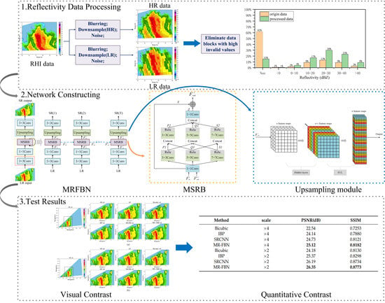
The upsampling block is a module used to change the input size of feature maps to a specified size. It is a key step in super-resolution reconstruction. The simplest upsampling method is interpolation. To tackle the limitations of traditional interpolation, a novel upsampling technique has been introduced, using a deconvolution layer. This layer increases image resolution by inserting zero-padded convolutions. This method has been applied successfully for visualizing layer activations [22] and semantic segmentation [23]. Dong et al. [24] first applied the deconvolution layer as an upsampling layer in the FSRCNN network, kickstarting the development of post-upsampling frameworks. However, the use of deconvolution, with its large number of zero-padding operations, can bring in invalid information and hinder gradient optimization, leading to the “uneven overlap” phenomenon [25]. This results in a checkerboard pattern, degrading SR performance. To address this issue, Shi et al. [26] proposed the ESPCN network, introducing the influential sub-pixel convolutional layer to increase the model’s receptive field and achieve HR feature maps via multi-channel recombination. Sub-pixel convolutional layers are now widely used in super-resolution tasks, leading to numerous successful network structures. However, uneven distribution of receptive fields may result in block regions sharing the same receptive field, causing artifacts near the boundaries of different block regions. Additionally, independently predicting neighboring pixels of blocky regions may lead to non-smooth output [27]. To resolve this, Gao et al. [28] proposed PixelTCL, a plug-and-play solution that replaces any transposed convolution and replaces independent predictions with interdependent sequential ones, yielding smoother and more consistent results. From this point of view, the current upsampling modules are aimed at simultaneous sampling in two directions, and it is important to find an effective unidirectional upsampling block.

3. Proposed Method

3.1. Network Structure

As depicted in Figure 2, the blue arrow represents the feedback connection. The MR-FBN architecture was proposed and can be unfolded into T iterations, where each iteration t is ordered temporally from 1 to T. To bring the hidden state in MR-FBN into play with the output, the loss at each iteration is tied. The sub-network in each iteration t consists of three parts: (1) a shallow feature extraction layer (represented by the red dotted line box in Figure 2). The features extracted by the shallow network are closer to the input and contain more pixel information. Although it contains more position and detail information, it has lower semantics and more noise due to fewer convolutions. (2) a deep feature extraction feedback layer (represented by the yellow dotted line box in Figure 2). The features extracted by the deep network are closer to the output and contain more abstract information. It mainly obtains data integrity information. (3) a reconstruction layer (represented by the blue dotted line box in Figure 2). The input and output of the network are defined as $I_{LR}$ and $I_{SR}$, respectively. Thus, the reconstruction process of the network model can be described as follows:

$$I_{SR}=H_{M{R}_{-}FBN}\left(I_{LR}\right)$$

(1)

where $H_{M{R}_{-}FBN}$ is our MR-FBN operation.

For a clearer understanding, the network structure is described as follows: We begin by extracting shallow features from the input low-resolution data using a 3 × 3 convolution. It is a simple convolution layer at the front of the entire network, which can obtain more local features and texture information from low-resolution data. This process can be represented as follows:

$$F_0^{\mathrm{t}}=f_{3\times 3}\left(I_{LR}\right)$$

(2)

where $F_0^{\mathrm{t}}$ is the shallow features extracted by 3 × 3 convolution, and $f_{3\times 3}$ denotes a convolution operation with a kernel size of 3 × 3 and a stride of 1.

Then the deep feature extraction layer consists of a 1 × 1 convolution and a feedback block. The purpose of the 1 × 1 convolution in the deep feature extraction layer is to perform feature reduction, and reduce the dimension to reduce the computational difficulty of the subsequent complex network structure. This helps to streamline subsequent feature calculations, minimize time costs and conserve computing resources. The use of the 1 × 1 convolution as a feature attenuation step ensures that the network remains efficient while still achieving its desired outcome. This process can be represented as follows:

$$F_{in}^t=f_{1\times 1}\left(F_0^t\right)$$

(3)

where $F_{in}^t$ is the feature maps after 1 × 1 convolution, and $f_{1\times 1}$ denotes a 1 × 1 convolution. The output of the feedback block will generate a hidden state, and the hidden state is then sent to the next iteration. The input of the feedback block in the next iteration will receive the hidden state generated in the previous iteration. This process can be represented as follows:

$$F_{\mathrm{out}}^t=f_{FB}\left([F_{\mathrm{out}}^{t-1},F_{\mathrm{in}}^t]\right)$$

(4)

where $f_{FB}$ represents the operations of the Feedback Block (FB), $[F_{\mathrm{out}}^{t-1},F_{\mathrm{in}}^t]$ represents the connection operation, in this article, MSRB (see Section 3.2 for details) is used as the feedback block to realize the function of transmitting information. $F_{\mathrm{out}}^{t-1}$ represents the hidden state from the previous iteration, and $F_{\mathrm{in}}^t$ represents the current input state.

The reconstruction layer operation is represented by $H_{REC}$. An upsampling module (as described in Section 3.3) was used to increase the resolution of the elevation angle, while maintaining the same distance resolution. The final step of the network uses a 3 × 3 convolution for reconstruction. The 3 × 3 convolution here mainly converts 64 channels into a standard format for 1-channel output through convolution, and can extract some feature information at the same time. This process can be represented as follows:

$$I_{SR}=H_{REC}\left(F_{\mathrm{out}}^t\right)$$

(5)

3.2. Multi-Scale Fusion Residual Block (MSRB)

To obtain more detailed features at various scales, we propose a Multi-scale Residual Block, as depicted in Figure 3. The details of its structure will be described in the following.

The utilization of large convolution kernels in a network is associated with an increased receptive field, leading to the detection of more intricate features. However, these large kernels are high in computational complexity and consume substantial computing resources and storage space. To address this issue, we propose a three-bypass network structure, where different bypasses utilize varying convolution kernels, with information shared among adjacent kernels. This approach limits the size of the convolution kernel span, reducing the use of larger kernels and enabling the detection of features at different scales, all while being easy to train. The feature fusion of the previous iteration’s output layer and the current input layer is achieved through a 1 × 1 convolution, as expressed below:

$$X=f_{1\times 1}\left([F_{\mathrm{in}}^t,F_{\mathrm{out}}^{t-1}]\right)$$

(6)

where X represents the output after 1 × 1 convolution, $F_{\mathrm{out}}^{t-1}$ represents the hidden state from the previous iteration, $F_{\mathrm{in}}^t$ represents the current input state, and represents a 1 × 1 convolution operation. Then, three feature vectors P1, Q1, and S1 are generated, respectively, through convolution with 3 × 3, 5 × 5, and 7 × 7 filters. The operation can be expressed as follows:

$$P1=\sigma \left(f_{3\times 3}^1\left(X\right)\right)$$

(7)

$$Q1=\sigma \left(f_{5\times 5}^1\left(X\right)\right)$$

(8)

$$S1=\sigma \left(f_{7\times 7}^1\left(X\right)\right)$$

(9)

where $f_{3\times 3}$, $f_{5\times 5}$, $f_{7\times 7}$ denote 3 × 3, 5 × 5, 7 × 7 convolution, respectively. The $\sigma$ symbol represents the Rectified Linear Unit (ReLU) activation function [29]. It introduces nonlinearity to enhance the expressive power of the network. And P1, Q1, and S1 feature vectors are then shared to generate new feature vectors. P1 and Q1 are concatenated and processed through a 3 × 3 convolution to generate P2, while P1 and S1 are concatenated and processed through a 5 × 5 convolution to generate Q2. Finally, Q1 and S1 are concatenated and processed through a 7 × 7 convolution to generate S2, which can be expressed as follows:

$$P2=\sigma \left(f_{3\times 3}^2\left([P1,Q1]\right)\right)$$

(10)

$$Q2=\sigma \left(f_{5\times 5}^2\left([P1,S1]\right)\right)$$

(11)

$$S2=\sigma \left(f_{7\times 7}^2\left([Q1,S1]\right)\right)$$

(12)

where [P1,Q1], [P1,S1], [Q1,S1] denote the connection operation. The feature vectors are connected and fused through the defined operations, as follows:

$$Z=f_{1\times 1}\left([P2,Q2,S2]\right)$$

(13)

To simplify the learning process and enhance the gradient propagation, we adopt the residual learning strategy. This strategy significantly reduces computational complexity and improves network performance, as expressed by the following equation:

$$F_{out}^t=X+Z$$

(14)

3.3. Upsampling Module

The task of enhancing the vertical structure resolution of weather radar echo is different from the traditional image super-resolution task. The current image super-resolution methods aim to improve both the height and width of an image, such as a 64 × 64 size image becoming 128 × 128 after ×2 super-resolution reconstruction. Our research, on the other hand, focuses on enhancing the elevation resolution while retaining the range resolution, such as a 64 × 64 size data becoming 64 × 128 after ×2 super-resolution reconstruction. This requirement makes the traditional upsampling layers inappropriate, which is why we propose an improved upsampling layer, referred to as the elevation upsampling layer (EUL).

Figure 4 shows the overall design of the Upsampling Block. It starts by applying a convolutional layer to expand the original n feature maps into $n\times r$ feature maps (n represents the number of feature maps and r represents the magnification). Subsequently, the EUL is utilized to rearrange the feature maps into the desired size. The mathematical expression for this module can be expressed as:

$$I_{\mathrm{output}}=f^L\left(I_{\mathrm{input}}\right)=PS\left(W\ast I_{\mathrm{input}}+b\right)$$

(15)

where $I_{\mathrm{input}}$ and $I_{\mathrm{output}}$ refer to the input and output of the Upsampling Block, and the Upsampling Block operation denoted by $f^L$. The new periodic shuffling operator, $PS$, rearranges the elements of a $H\times W\times C\times r$ tensor into a tensor of shape $rH\times W\times C$. The impact of this operation is demonstrated in Figure 4. The EUL is based on the original image sub-pixel convolutional layer [27]. During the convolution of the filter on the feature map, these modes are periodically activated, depending on the position of the sub-data: (mod(x,r), y), where x and y are the output data coordinates in the HR space, and r is the magnification factor. Mathematically, this operation can be expressed as follows:

$$PS{\left(T\right)}_{x,y,c}=T_{\lfloor x/r\rfloor ,\lfloor y\rfloor ,mod(x,r)+c}$$

(16)

The process of arranging the positions of multiple feature maps on one feature map to obtain an enlarged feature map is achieved through the modulo operation. Taking r = 4 as an example, the first row of the first, second, third, and fourth feature maps of low resolution are, respectively, arranged in the first row of the first feature map of high resolution, and the first row of the feature map of the first Second row, third row and fourth row. The second row of the first, second, third, and fourth low-resolution feature maps are arranged in the fifth, sixth, seventh, and seventh rows of the high-resolution first feature map, respectively, eight lines. By following this pattern, the enlarged feature map as shown in Figure 4 (EUL) can be obtained.

4. Experiment

4.1. Datasets and Metrics

The experimental data were obtained from the basic reflectivity data of the RXM-25 radar RHI scan collected between June to October 2020 and June to October 2021. As shown in Figure 5, RXM-25 radar is produced by Colorado State University and has a dual polarization. Doppler weather radar operating in the x-band with a range coverage of approximately 50 km, and its relevant technical indicators are shown in

Table 1. Main parameters of RXM-25 radar.

Parameter	Min	Typ	Max	Unit
Frequency	9380	9410	9440	MHz
Peak Output Power	18.0	18.5	25.0	kW
Duty Cycle		0.15	0.16	%
Pulse Width	100	660	2000	ns
Range sampling interval		60		m
Elevation angle interval	0.1		0.3	°

. Its high sampling resolution provides advanced polarization radar data products. We used the RHI data with a range resolution of 60 m, a maximum range of 66 km, and elevations between 2.0 and 59.8°. The low-resolution (LR) data were simulated using the VCP11 (0.5°, 1.45°, 2.4°, 3.35°, 4.3°, 5.25°, 6.2°, 7.5°, 8.7°, 10.0°, 12.0°, 14.0°, 16.7°, 19.5°). However, due to the blocking of the buildings around the radar, data for 0.5° and 1.45° could not be detected, and only 12 elevation angle data were used as the LR input. For the production of the label ×2HR corresponding to the input data, we use the 14 elevation angles of VCP11 as the basis, and take the central angle between the elevation angles as the central elevation angle. Due to occlusion, we only need 24 elevation angles. The label production of ×4HR is based on the elevation angle of ×2HR, and then the central angle between the elevation angles is taken as the central elevation angle; finally, 48 elevation angle data are obtained. LR data are used as the input for the proposed super-resolution algorithm, which is reconstructed through super-resolution to obtain high-resolution datasets of 24 (×2SR) and 48 (×4SR) elevation angles. The performance of the proposed algorithm can be objectively evaluated by comparing the similarity between the original data and the high-resolution dataset.

Radar data can contain invalid values due to blocking during the detection process. We performed basic reflectivity statistics on the initial LR dataset and found that the proportion of invalid values differed greatly from other reflectivity values (as shown in the yellow bar chart in Figure 6). This would cause the network model to learn more characteristics of the invalid regions. Therefore, we preprocessed the initial LR dataset by cutting it to 32 in the distance direction with a step size of 10, resulting in 12 × 32. Second, if the number of invalid values in a data block was less than two-thirds of the total, it was stored in the dataset, otherwise, it was discarded as bad data. The basic reflectivity statistics of the processed dataset are shown in the green bar chart in Figure 6, the proportion of inefficiencies has been significantly reduced.

The high-resolution dataset is generated from the low-resolution dataset by preserving the information. The block size for the ×2HR data is 24 × 32 and for the ×4HR data is 48 × 32. Finally, the basic reflectivity value of the dataset is converted to the 0–255 range through Formula (17) to simulate a grayscale pixel value, which expands the dynamic range and can help the network learn features such as texture, shape, and structure of radar data.

$$R^{\prime }=33+2\times R$$

(17)

$R^{\prime }$ refers to the basic reflectivity value that has been mapped to a range of 0–255, while R refers to the original basic reflectivity value. To evaluate the performance of super-resolution reconstruction, we use two metrics: Peak Signal to Noise Ratio (PSNR) and Structural Similarity (SSIM) [30]. The formula for PSNR is as follows:

$$PSNR=10·{log}_{10}\left(\frac{R_{max}^2}{MSE}\right)$$

(18)

$$MSE=\frac{1}{mn}\sum _{i=0}^{m-1}\sum _{j=0}^{n-1}{\left[I^{HR}(i,j)-I^{SR}(i,j)\right]}^2$$

(19)

where $R_{max}$ represents the maximum reflectivity, MSE is the mean square error between the reconstructed data value and the actual data value, while HR data are denoted by $I^{HR}$, SR data by $I^{SR}$, and m and n represent the height and width of the data, respectively. A higher value of PSNR indicates better reconstruction performance, while a lower value means worse performance. Since PSNR only considers the error between the original echo and the reconstructed echo, it only pays attention to the details of the reconstructed structure, and ignores the structural similarity in human perception, especially in data with complex structures. In contrast, SSIM is more in line with human perception to evaluate the quality of reconstruction results, considering global and local features, especially the degree of preservation of structural information. Therefore, this paper adds the SSIM index to judge the structural characteristics of the echo. The SSIM formula is given as follows:

$$SSIM(x,y)=\frac{\left(2{\mu }_x{\mu }_y+c_1\right)\left(2{\sigma }_{xy}+c_2\right)}{\left({\mu }_x^2+{\mu }_y^2+c_1\right)\left({\sigma }_x^2+{\sigma }_y^2+c_2\right)}$$

(20)

where x, y denotes SR data and HR data, respectively, ${\mu }_x$, ${\sigma }_x^2$ are mean and variance of x, ${\mu }_y$, ${\sigma }_y^2$ are mean and variance of y, ${\sigma }_{xy}$ is the covariance of x and y. $c_1$ and $c_2$ are constants used to make the calculation more stable and prevent the denominator from being too small. The SSIM is used to evaluate the reconstruction performance, with a value closer to 1 indicating a better performance and a value closer to 0 indicating a worse performance.

4.2. Implementation Details

The block size of the low-resolution (LR) data is 12 × 32, while the HR data blocks have dimensions of 24 × 32 and 48 × 32 for ×2 HR and ×4 HR, respectively. During the training process, we set the batch size to 64 and use the Adam optimizer, with hyperparameters $\beta 1=0.9$, $\beta 2=0.99$, $\epsilon ={10}^{-8}$ [31], to optimize MR-FBN. The learning rate is set to $1\times {10}^{-4}$. To optimize MR-FBN, we choose L1 loss as the primary objective function, which is widely used in super-resolution algorithms [32]. The loss function in MR-FBN calculates the absolute value error between each iteration’s output and the real value, and then the final objective function is determined by taking a weighted average of these values and averaging over all training samples, where $\theta$ denotes the network parameters to be learned by minimizing the loss between the reconstructed data F(Y; $\theta$) and the corresponding high-resolution data X. Given a set of high-resolution data $\left\{X_i\right\}$ and a corresponding set of low-resolution data $\left\{X_i\right\}$, we use the following formula as the loss function.The mathematical expression for the loss function in the network can be represented as:

$$L\left(\theta \right)=\frac{1}{n}\sum _{i=1}^n\left(\frac{1}{T}\sum _{t=1}^T{W}^{\left(t\right)}{∥F^{\left(t\right)}\left(Y_i;\theta \right)-X_i∥}_1\right)$$

(21)

where $\theta$ is the parameter of MR-FBN. $W^{\left(t\right)}$ is a weighted factor that demonstrates the worth of the output at the t-th iterations. T represents the number of iterations. In line with the approach presented in [32], we set the output value of each iteration to 1, indicating that each output contributes equally. n is the number of training samples.

As demonstrated in [33], the reconstruction quality continues to improve as the number of iterations increases. To strike a balance between the reconstruction quality and computational resources, we set the number of iterations T to 4. Additionally, the filter size is set to 64. All experiments in this paper were performed using the PyTorch [34].

4.3. Comparison with Existing Technology

To evaluate the effectiveness of the proposed network model, MR-FBN, we compare it with three commonly used methods: bicubic interpolation, IBP [16], and SRCNN [13]. The interpolation operation for IBP and SRCNN was modified to only interpolate in height while keeping the width unchanged to suit the specific requirements of this task. The comparison was carried out using the same training and test sets to ensure a fair evaluation of their reconstruction performance.

4.3.1. Visual Comparison

Considering the importance of weather radar reflectivity maps to forecasters and researchers, we visualized the vertical structure data to evaluate the reconstruction performance. Three vertical structural data samples with azimuth angles of 172.0° on 29 August 2020, 218.4° on 7 July 2021, and 73.0° on 26 July 2021, have been selected for visual analysis, referred to as Case 1, Case 2, and Case 3, respectively. Here we test the data within the entire detection range, and do not handle invalid values. The LR echo is used as the input of super-resolution reconstruction, and the high-resolution echo is obtained using the method of interpolation/reconstruction/learning. The scaling factors are ×2 and ×4. Scaling factor ×2 means that the number of vertical scanning elevation angles is increased by two times, and the distance resolution remains unchanged at 60 m; scaling factor ×4 means that the number of vertical scanning elevation angles is increased by four times, and the distance resolution remains unchanged at 60 m.

As seen in Figure 7, Figure 8 and Figure 9, the vertical structure data reconstructed by bicubic interpolation is visibly distorted and contains many artifacts. While the IBP method shows some improvement, it still fails to address the problem of edge diffusion. The use of the deep learning method, SRCNN, has significantly improved the reconstruction compared to the previous methods, which demonstrates the potential of deep learning for this task. However, the echo structure reconstructed by the MR-FBN method proposed in this paper is closest to the high-resolution echo structure, and the reconstruction quality of edge texture features in both strong echo and weak echo areas is higher, and artifacts and false echoes are relatively fewer. Especially under the ×2 scaling factor, not only is the strong echo area closer to the original data, but the edge diffusion phenomenon is also greatly suppressed, and detailed information on the strong echo area can be recovered as much as possible.

To show more clearly where the proposed method has relatively better results, we divide the reflectivity interval into five intervals of 0–10, 10–20, 20–30, 30–40, and >40 for comparison and obtain PSNR values of different methods in each interval.

It can be seen from the Figure 10, Figure 11 and Figure 12 that in the reflectivity interval without stray area interference, they all have relatively high PSNR values. It can be seen that the proposed method has a relatively good reconstruction effect for the intervals of 20–30, 30–40, and >40, i.e., the interval with a reflectivity greater than 20 dBZ. These areas usually correspond to disastrous weather processes such as strong convection, and can effectively reflect the evolution of weather processes. Therefore, the proposed method has a better PSNR value than the traditional bicubic interpolation method, IBP, and SRCNN is more effective for the regional reconstruction of key meteorological elements. At the same time, the proposed method can effectively reconstruct the vertical structure of the radar echo in a more refined weather process in the strong echo area, which is of great significance to the understanding of the evolution of weather and meteorological services, such as forecasting and early warning. However, the PSNR in the weak echo area has not improved much, and it may be lower than SRCNN (Case3). We guess that the preprocessing interpolation operation of SRCNN may have some advantages in the weak echo area, and we can follow this in future research.

4.3.2. Quantitative Results

To further verify the effectiveness of the proposed method, we tested the PSNR and SSIM values of the entire detection area.

Table 2. Comparison with existing methods.

Method	Scale	PSNR (dB)	SSIM
Bicubic	×4	22.54	0.7253
IBP	×4	24.14	0.7880
SRCNN	×4	24.73	0.8121
MR-FBN	×4	25.12	0.8182
Bicubic	×2	24.18	0.8130
IBP	×2	25.37	0.8298
SRCNN	×2	26.19	0.8734
MR-FBN	×2	26.35	0.8773

The best results are bold.

displays the results at ×2 and ×4 super-resolution. The bolded values indicate the best performance under similar conditions. It can be seen that our method has significantly better PSNR and SSIM values than bicubic interpolation and IBP. Compared with the interpolation method commonly used in the meteorological field, our method can improve by about 2 dB. Compared with SRCNN, there is also a certain improvement. The results show that our method can extract more complex features from LR radar echoes. When the magnification is larger, more information needs to be reconstructed, while the LR radar echo contains relatively less information, resulting in the loss of most high-frequency information, making it difficult to reconstruct better performance results. This leads to the reconstruction performance of ×4 is not as good as that of ×2.

5. Conclusions

This paper proposes a convolutional neural network that can refine the vertical structure of radar echoes without occupying radar resources. To improve the feature extraction ability of the network, the network result constructs a multi-scale residual block, which can carry out multi-scale feature information sharing, which not only reduces the network parameters but also obtains more accurate feature extraction. At the same time, the feedback network is used as the overall framework, and the refined information iterated step-by-step is used to guide the reconstruction of more refined results to achieve feature reuse, which can not only maintain the diversity of feature maps but also improve network performance. Experiments show that MR-FBN is a network model suitable for the reconstruction of radar echo vertical structure data, which can reconstruct data closer to the original radar echo in a visual effect. In quantitative analysis, compared with interpolation and reconstruction, the method has obvious improvements, but compared with SRCNN, which is also a neural network, the performance improvement is not particularly great. This may be due to (1) a small amount of data. Since the RHI scan mode is a non-standard mode, the amount of data is relatively small. (2) The particularity of the task. Our radar echo vertical structure refinement task is the number of elevation angles, i.e., the resolution in only one direction is increased, so there is relatively little space for performance improvement. The refined vertical structure of radar echoes is crucial for understanding the complex microphysical processes of clouds and precipitation, and providing necessary data support for studying the formation, evolution, and dissipation of low-level wind shear and turbulence. In the future, we will enrich our database and obtain more effective data for network learning feature information. At the same time, this task is crucial for the in-depth study of the generation and elimination process of disastrous weather. It is important to explore super-resolution reconstruction networks suitable for the vertical structure of radar echoes. We will explore more network frameworks, such as Recurrent Neural Networks(RNN), Generative Adversarial Networks(GAN), etc.

References

1. Liu, J.; Huang, X.; He, Y.; Wang, Z.; Wang, J. Comparison and Analysis of X-band Phased Array Weather Radar Echo Data. Plateau Meteorol. 2015, 34, 1167–1176. [Google Scholar]
2. Lim, S.; Allabakash, S.; Jang, B.; Chandrasekar, V. Polarimetric radar signatures of a rare tornado event over South Korea. J. Atmos. Ocean. Technol. 2018, 35, 1977–1997. [Google Scholar] [CrossRef]
3. Cho, J.Y.; Kurdzo, J.M. Weather radar network benefit model for tornadoes. J. Appl. Meteorol. Climatol. 2019, 58, 971–987. [Google Scholar] [CrossRef] [Green Version]
4. Huang, C.; Zhang, A.; Chen, S.; Hu, B. Comparison of GPM Satellite and Ground Radar Estimation of Tornado Heavy Precipitation in Yancheng, Jiangsu. J. Atmos. Sci. 2020, 43, 370–380. [Google Scholar]
5. Chen, D.; Chen, G.; Wu, Z. Combination RHI Automatic Realization Algorithm Based on Volume Scan Mode. Meteorological 2010, 36, 109–112. [Google Scholar]
6. Liu, Y.; Gu, S.; Zhou, Y.; Zhang, S.; Dai, Z. Comparison and Analysis of Volume Scan Models of New Generation Weather Radar. Meteorological 2006, 32, 44–50. [Google Scholar]
7. Zhang, Y.; Zhao, D.; Zhang, J.; Xiong, R.; Gao, W. Interpolation-dependent image downsampling. IEEE Trans. Image Process. 2011, 20, 3291–3296. [Google Scholar] [CrossRef]
8. Thévenaz, P.; Blu, T.; Unser, M. Image interpolation and resampling. Handb. Med. Imaging Process. Anal. 2000, 1, 393–420. [Google Scholar]
9. Qiu, D.; Zheng, L.; Zhu, J.; Huang, D. Multiple improved residual networks for medical image super-resolution. Future Gener. Comput. Syst. 2021, 116, 200–208. [Google Scholar] [CrossRef]
10. Guo, K.; Guo, H.; Ren, S.; Zhang, J.; Li, X. Towards efficient motion-blurred public security video super-resolution based on back-projection networks. J. Netw. Comput. Appl. 2020, 166, 102691. [Google Scholar] [CrossRef]
11. Huang, Y.; Shao, L.; Frangi, A.F. Simultaneous super-resolution and cross-modality synthesis of 3D medical images using weakly-supervised joint convolutional sparse coding. In Proceedings of the IEEE Conference on Computer Vision and Pattern Recognition, Honolulu, HI, USA, 21–26 July 2017; pp. 6070–6079. [Google Scholar]
12. Dong, C.; Loy, C.C.; He, K.; Tang, X. Learning a deep convolutional network for image super-resolution. In Part IV 13, Proceedings of the Computer Vision–ECCV 2014: 13th European Conference, Zurich, Switzerland, 6–12 September 2014; Springer: New York, NY, USA, 2014; pp. 184–199. [Google Scholar]
13. Torres, S.M.; Curtis, C.D. 5B. 10 Initial Implementation of Super-Resolution Data on the Nexrad Network. Available online: https://ams.confex.com/ams/87ANNUAL/techprogram/paper_116240.htm (accessed on 27 December 2022).
14. Yao, H.; Wang, J.; Liu, X. Minimum Entropy Spectral Extrapolation Technique and Its Application in Radar Super-resolution. Mod. Radar 2005, 27, 18–19. [Google Scholar]
15. Gallardo-Hernando, B.; Munoz-Ferreras, J.; Pérez-Martınez, F. Super-resolution techniques for wind turbine clutter spectrum enhancement in meteorological radars. IET Radar Sonar Navig. 2011, 5, 924–933. [Google Scholar] [CrossRef]
16. He, J.; Ren, H.; Zeng, Q.; Li, X. Super-Resolution reconstruction algorithm of weather radar based on IBP. J. Sichuan Univ. (Nat. Sci. Ed.) 2014, 51, 415–418. [Google Scholar]
17. Wu, Y.; Zhang, Y.; Zhang, Y.; Huang, Y.; Yang, J. TSVD with least squares optimization for scanning radar angular super-resolution. In Proceedings of the 2017 IEEE Radar Conference (RadarConf), Seattle, WA, USA, 8–12 May 2017; IEEE: New York, NY, USA, 2017; pp. 1450–1454. [Google Scholar]
18. Tan, K.; Li, W.; Zhang, Q.; Huang, Y.; Wu, J.; Yang, J. Penalized maximum likelihood angular super-resolution method for scanning radar forward-looking imaging. Sensors 2018, 18, 912. [Google Scholar] [CrossRef] [Green Version]
19. Zeng, Q.; He, J.; Shi, Z.; Li, X. Weather radar data compression based on spatial and temporal prediction. Atmosphere 2018, 9, 96. [Google Scholar] [CrossRef] [Green Version]
20. Zhang, X.; He, J.; Zeng, Q.; Shi, Z. Weather radar echo super-resolution reconstruction based on nonlocal self-similarity sparse representation. Atmosphere 2019, 10, 254. [Google Scholar] [CrossRef] [Green Version]
21. Yuan, H.; Zeng, Q.; He, J. Weather Radar Image Superresolution Using a Nonlocal Residual Network. J. Math. 2021, 2021, 4483907. [Google Scholar] [CrossRef]
22. Zeiler, M.D.; Fergus, R. Visualizing and understanding convolutional networks. In Part I 13, Proceedings of the Computer Vision–ECCV 2014: 13th European Conference, Zurich, Switzerland, 6–12 September 2014; Springer: New York, NY, USA, 2014; pp. 818–833. [Google Scholar]
23. Long, J.; Shelhamer, E.; Darrell, T. Fully convolutional networks for semantic segmentation. In Proceedings of the IEEE Conference on Computer Vision and Pattern Recognition, Boston, MA, USA, 7–12 June 2015; pp. 3431–3440. [Google Scholar]
24. Dong, C.; Loy, C.C.; Tang, X. Accelerating the super-resolution convolutional neural network. In Part II 14, Proceedings of the Computer Vision–ECCV 2016: 14th European Conference, Amsterdam, The Netherlands, 11–14 October 2016; Springer: New York, NY, USA, 2016; pp. 391–407. [Google Scholar]
25. Odena, A.; Dumoulin, V.; Olah, C. Deconvolution and checkerboard artifacts. Distill 2016, 1, e3. [Google Scholar] [CrossRef]
26. Shi, W.; Caballero, J.; Huszár, F.; Totz, J.; Aitken, A.P.; Bishop, R.; Rueckert, D.; Wang, Z. Real-time single image and video super-resolution using an efficient sub-pixel convolutional neural network. In Proceedings of the IEEE Conference on Computer Vision and Pattern Recognition, Las Vegas, NV, USA, 27–30 June 2016; pp. 1874–1883. [Google Scholar]
27. Wang, Z.; Chen, J.; Hoi, S.C. Deep learning for image super-resolution: A survey. IEEE Trans. Pattern Anal. Mach. Intell. 2020, 43, 3365–3387. [Google Scholar] [CrossRef] [Green Version]
28. Gao, H.; Yuan, H.; Wang, Z.; Ji, S. Pixel transposed convolutional networks. IEEE Trans. Pattern Anal. Mach. Intell. 2019, 42, 1218–1227. [Google Scholar] [CrossRef] [PubMed]
29. Agarap, A.F. Deep learning using rectified linear units (relu). arXiv 2018, arXiv:1803.08375. [Google Scholar]
30. Horé, A.; Ziou, D. Image Quality Metrics: PSNR vs. SSIM. In Proceedings of the 2010 20th International Conference on Pattern Recognition, Milan, Italy, 23–26 August 2010; pp. 2366–2369. [Google Scholar] [CrossRef]
31. Kingma, D.P.; Ba, J. Adam: A method for stochastic optimization. arXiv 2014, arXiv:1412.6980. [Google Scholar]
32. Wang, S.; Zhou, T.; Lu, Y.; Di, H. Contextual transformation network for lightweight remote-sensing image super-resolution. IEEE Trans. Geosci. Remote. Sens. 2021, 60, 1–13. [Google Scholar] [CrossRef]
33. Li, Z.; Yang, J.; Liu, Z.; Yang, X.; Jeon, G.; Wu, W. Feedback network for image super-resolution. In Proceedings of the IEEE/CVF Conference on Computer Vision and Pattern Recognition, Long Beach, CA, USA, 15–20 June 2019; pp. 3867–3876. [Google Scholar]
34. Paszke, A.; Gross, S.; Chintala, S.; Chanan, G.; Yang, E.; DeVito, Z.; Lin, Z.; Desmaison, A.; Antiga, L.; Lerer, A. Automatic Differentiation in Pytorch. 2017. Available online: https://openreview.net/forum?id=BJJsrmfCZ (accessed on 27 December 2022).
Figure 1. Schematic diagram of VCP11 and VCP21 scanning strategy.
Remotesensing 15 03676 g001
Figure 2. The overall structure of MR-FBN.
Remotesensing 15 03676 g002
Figure 3. The structure of a multi-scale fusion residual block (MSRB).
Remotesensing 15 03676 g003
Figure 4. Upsampling Block: a convolutional layer is used to extract features, and an improved sub-pixel convolutional layer is used to aggregate feature maps in LR space.
Remotesensing 15 03676 g004
Figure 5. RXM-25 Radar.
Remotesensing 15 03676 g005
Figure 6. Reflectivity distribution, yellow denotes the original data, green denotes the processed data.
Remotesensing 15 03676 g006
Figure 7. Case1 Visual comparison with other methods on ×2SR (a) and ×4SR (b).
Remotesensing 15 03676 g007
Figure 8. Case2 Visual comparison with other methods on ×2SR (a) and ×4SR (b).
Remotesensing 15 03676 g008
Figure 9. Case3 Visual comparison with other methods on ×2SR (a) and ×4SR (b).
Remotesensing 15 03676 g009
Figure 10. Case1 Comparison of different methods in different reflectivity intervals on ×2SR (a) and ×4SR (b).
Remotesensing 15 03676 g010
Figure 11. Case2 Comparison of different methods in different reflectivity intervals on ×2SR (a) and ×4SR (b).
Remotesensing 15 03676 g011
Figure 12. Case3 Comparison of different methods in different reflectivity intervals on ×2SR (a) and ×4SR (b).
Remotesensing 15 03676 g012