Article

Magnetotelluric Deep Learning Forward Modeling and Its Application in Inversion

College of Computer Science and Cyber Security, Chengdu University of Technology, Chengdu 610059, China
*
Author to whom correspondence should be addressed.
Remote Sens. 2023, 15(14), 3667; https://doi.org/10.3390/rs15143667
Submission received: 22 June 2023 / Revised: 10 July 2023 / Accepted: 17 July 2023 / Published: 23 July 2023

Abstract

:
Magnetotelluric (MT) inversion and forward modeling are closely linked. The optimization and iteration processes of the inverse algorithm require frequent calls to forward modeling. However, traditional numerical simulations for forward modeling are computationally expensive; here, deep learning (DL) networks can simulate forward modeling and significantly improve forward speed. Applying DL for forward modeling in inversion problems requires a high-precision network capable of responding to fine changes in the model to achieve high accuracy in inversion optimization. Most existing MT studies have used a convolutional neural network, but this method is limited by the receptive field and cannot extract global feature information. In contrast, the Mix Transformer has the ability to globally model and extract features. In this study, we used a Mix Transformer to hierarchically extract feature information, adopted a multiscale approach to restore feature information to the decoder, and eliminated the skip connection between the encoder and decoder. We designed a forward modeling network model (MT-MitNet) oriented toward inversion. A sample dataset required for DL forward was established using the forward data generated from the traditional inverse calculation iteration process. The trained network quickly and accurately calculates the forward response. The experimental results indicate a high agreement between the forward results of MT-MitNet and those obtained with traditional methods. When MT-MitNet replaces the forward computation in traditional inversion, the inversion results obtained with it are also highly in agreement with the traditional inversion results. Importantly, under the premise of ensuring high accuracy, the forward speed of MT-MitNet is hundreds of times faster than that of traditional inversion methods in the same process.

Graphical Abstract

1. Introduction

Magnetotelluric (MT) inversion is a branch of geophysics, and inversion is a method used to determine the corresponding geophysical model (resistivity) from given observations (apparent resistivity and phase). Since the 1950s when the MT method was introduced, MT inversion methods have been playing an important role in various applications, including marine geophysics, environmental geophysics, understanding the electrical structure of the Earth’s crust and upper mantle, geological exploration, and mineral exploration [1,2].
Inversion algorithms can be categorized into indirect inversion and direct inversion based on the relationship between data and models. Indirect inversion requires an initial model and boundary conditions to use iterative optimization methods to find the minimum fitting difference after multiple iterations. Occam inversion [3,4], rapid relaxation inversion [5], nonlinear conjugate gradient inversion [6,7], and Gauss–Newton inversion [8,9] are frequently utilized in the MT inversion of the Earth because of their high accuracy and computational stability, although their efficiency and speed are lower. Direct inversion techniques, on the other hand, perform forward approximations to determine the relationship between field values and models and require no initial model to produce inversion results. Nonlinear direct inversion methods such as the BOSTICK inversion [10] algorithm, genetic algorithm, and artificial neural network (ANN) [11] can enhance efficiency; however, their inversion accuracy and stability are restricted, necessitating further development and improvement.
The exponential growth in computing technology has led to the increased use of ANNs and DL research methods in the field of MT. In contrast to the conventional linearized inversion theory approach, the DL-based MT approach involves creating sample datasets, designing and training specific network models, and ultimately achieving fast prediction from data models of the results. The computational efficiency of the model to the result is greatly improved when the network training reaches convergence. For instance, Fang et al. [12] improved the overall quality of inversion on low-frequency seismic data modules using an ANN. Similarly, Moseley et al. [13] predicted the response velocity of acoustic and seismic waves generated in a horizontally layered medium using an ANN. Hansen and Cordua [14] utilized DL to rapidly calculate the forward response for improved efficiency in the inversion of ground-penetrating radar datasets. Li et al. [15] trained an end-to-end ANN to invert the velocity model, fully utilizing the feature information from seismic data. Puzyrev [16] demonstrated the significant potential of deep learning in inversion by predicting resistivity distributions using trained NNs with deeper and more complex layers on small datasets. Puzyrev and Swidinsky [17] discovered that a complex NN could extract richer feature information and predict accurate results but is often expensive to train and does not generalize well. Liu et al. [18] constructed a theoretically driven one-dimensional DL magnetotelluric inversion, but the DL inversion produces low-precision EM responses and cannot be used in two-dimensional geoelectric inversion. Conway et al. [19] accelerated MT inversion by utilizing neural networks for forward computation. However, the anomalies in training geoelectric models were relatively simple, and the average accuracy of the network was only 70%. Liu et al. [20] used a U-shaped neural network architecture for the inversion of resistivity data, whereas Guo et al. [21] applied a supervised descent method along with a priori information to accelerate the inversion process for transient electromagnetic data. However, they used neural networks with less complex layers and structures, and the sample datasets of the networks were artificially generated rather than being obtained based on inversion algorithms. Therefore, it was difficult for the trained network models to have strong generalization ability and higher accuracy.
Although traditional MT forward modeling calculations are highly accurate, they are time-consuming and inefficient. Additionally, the inversion process necessitates multiple calls to forward modeling calculations and multiple iterations to determine the most optimal solution. In contrast to inversion, forward modeling does not offer multiple solutions. Deep learning can approximate the nonlinear mapping relationship of forward modeling, thus enabling quicker prediction from the model to results and enhancing efficiency. This increased efficiency is advantageous for inversion calculations that depend on forward modeling as a vital parameter to solve the problem. As such, the network model should possess a broader receptive field, powerful global modeling capability, and an accurate response to small model changes, allowing for high prediction accuracy in the forward modeling results. Based on experimental results, the main contributions of this article are:
1.
The construction of a new forward network dataset to serve MT inversion. To ensure the effectiveness of DL networks, constructing an appropriate dataset for the training samples is crucial for MT forward networks. The inverse forward response model is generated iteratively through an optimization algorithm during the inversion procedure, which differs from real subsurface models or human-made models. We used different geoelectric models for MT forwarding and input the inversion program after obtaining the observed data. By acquiring the forward data generated by the inversion process to build a forward sample dataset that fits the inversion iterative model, an excellent forward network model oriented to inversion was trained.
2.
We designed the forward modeling network MT-MitNet for forward computations. MT-MitNet takes Mix Transformer [22] as the backbone of the network, obtains rich feature information of the anomalies in the encoding module, reconstructs anomalous features in the decoding module by combining multiscale ideas, and eliminates the skip connection between the encoder and decoder. After training, MT-MitNet, with global modeling capability, displayed stable and rapid forward modeling calculations, with an average accuracy greater than 95%. MT-MitNet serves the forward calculation in inversion with high accuracy, which improves the overall efficiency of inversion calculation, and the network model has strong generalization ability in the face of multiple anomalies.

2. Methodology

2.1. Dataset Preparation

Preparing sample data is a key step in conducting research on deep learning network models. In the field of computer vision, training networks often use abundant, accurately labeled, and open-source datasets. However, for MT data, it is quite difficult to obtain millions of actual samples. It is worth noting that traditional inversion algorithms, such as the Occam inversion, require a large number of forward computations to reduce the fitting error during the iterative process of inversion computation searching. The data generated by this process (apparent resistivity, phase, and resistivity models) are produced by the inversion algorithm, providing a highly accurate sample for deep-learning-based forward modeling networks. This not only avoids the uncertainty of manually produced forward modeling samples but also facilitates more effective training of the forward modeling network models. The Occam inversion algorithm is based on the idea of smooth inversion to achieve smooth inversion results with strong stability. However, the required multiple forward computations result in time-consuming and inefficient computation. In this study, we utilized the Occam inversion method as an example to conduct experiments on the forward computation process within the deep learning replacement inversion algorithm. The aim was to predict high-precision forward results through deep learning networks and to use them in inversion computation.
In actual engineering environments, the subsurface model is varied within a certain range. The two-dimensional geoelectric model simulated in this study was 4096 m in length and 1024 m in height, with a frequency range between 10 2 and 10 2 , and the number of frequency points was set to 32. The observation points were spaced 32 m apart, and the number of measurement points was set to 128 so that the size of both the simulated geoelectric model and the original observation data was 32 × 128. The anomalies were located in a homogeneous half-space and consisted of positive circles, ellipses, and arbitrary (shaped) closed figures with random distribution locations and resistivity values between 10 2 and 10 4 Ω m with a background resistivity of 100 Ω m.
The process of producing the sample database for the MT-inversion-oriented forward network model is shown in Figure 1. The anomalous body dataset comprises 7 anomalous body categories, each divided into 1000 groups based on location in space and resistivity value. Initially, an anomalous body sample is selected from the dataset, which is subjected to MT forward calculation to obtain the apparent resistivity and phase results. These results constitute the observed data necessary for standard Occam inversion calculation. During the iterative process of the Occam inversion algorithm, forward data are generated and saved, and ten data groups are selected randomly and saved in the dataset. The aforementioned process is repeated for each sample set, resulting in a total of 70,000 groups of forward data.

2.2. Inversion-Oriented Deep Learning Forward Network Model: MT-MitNet

In practical applications of MT inversion, people are more concerned about the size and electrical characteristics of the anomalous bodies. For the inversion results, they hope to accurately determine the resistance value of the anomaly and the boundary situation of the anomaly delineated from the surrounding normal rock. In the last decade, many researchers have conducted MT forward and inverse studies using recurrent neural networks (RNNs) [23,24] or convolutional neural networks (CNNs) [25,26,27,28]. The MT forward results have no obvious edges, and the global information is quite important, but RNNs cannot effectively capture the data-dependent information of ultra-long sequences, and the parallelized computational capability is less efficient and more time-costly. The convolution in CNNs is limited by the perceptual field size and has the problems of translation invariance and focusing only on local information, making it difficult to establish global information at a larger scale. The network model based on the Transformer [29] architecture improves these problems, and the Transformer is able to perform parallel computation and process more information in less time, making up for the lower efficiency of RNNs in parallel computation. Additionally, the Transformer utilizes a self-attention mechanism, showcasing exceptional learning ability and parallel performance in the processing of sequential data. As a result of this self-attention mechanism being present, the encoding module possesses a larger effective receptive field in comparison with traditional CNN encoders. This allows Transformer-based models to acquire a more comprehensive range of global information while possessing dynamic global modeling capabilities. It can capture information regarding global features and compensate for the limitations of convolutional neural networks in acquiring global information. Based on the excellent performance of the Transformer architecture, Vision Transformer (ViT) [30] and Mix Transformer (MiT) [22] for two-dimensional data have emerged one after another. ViT transforms the input information into vectors, and key features may be ignored, while MiT comprises a hybrid attention module based on ViT architecture, which uses a hierarchical extraction mechanism to obtain feature map information, and it is able to pay attention to both feature extraction and target information integration and has a simple structure and higher efficiency. Considering the various sizes and spatial distributions of anomalies, the magnetoelectric method places great emphasis on achieving accurate overall results. Interactions exist among multiple anomalies within a specific area, and the inversion process entails conducting numerous forward calculations and iterative optimization to obtain the optimal model. The network model should accurately and effectively extract as much feature information about the anomalies as possible. Moreover, using deep learning for forward simulation and applying it in inversion requires a network with high computational precision to accurately respond to small model modifications. MiT has self-attention and hierarchical feature extraction mechanisms, and its receptive field is larger than that of traditional CNNs, allowing it to capture more detailed and complete feature information.
The importance of global information and the need for accuracy led us to choose MiT with global modeling capabilities as the backbone of the network. In addition, MiT has a skip-connection structure that superimposes feature information from the encoding module onto the corresponding decoding module. But the magnetoelectric forward simulation results are progressively smoothers, without obvious edges and without requiring redundant superimposition of feature information. The skip-connection structure incorporates the preserved anomalous data and excessive edge information from the encoding module into the forward result [31], leading to inadequate smoothness in the forward results. Therefore, we removed the skip-connection structure between the encoding and decoding modules. Considering the characteristics of forward and inversion MT data, the forward network model MT-MitNet for MT inversion is proposed based on Mix Transformer with low computation and hierarchical extraction of features, as shown in Figure 2.
MT-MitNet consists of an encoding module and a decoding module. The encoding module consists of 4 Mix Transformer Blocks (MiT-Blocks); each MiT-Block consists of efficient self-attention module, mix feed-forward network (Mix-FFN) module, and overlapped patch-merging module. The hierarchical coding module in MiT achieves global modeling through a self-attentive mechanism. The Mix-FFN mainly consists of two lightweight multilayer perceptrons (MLPs), GELU activation, and a 3 × 3 convolution layer. Meanwhile, the Mix-FFN utilizes the translation invariance of convolution operations to incorporate location information into the Mix Transformer. This approach offers increased flexibility compared with the location coding of the original Transformer. The structure of Mix Transformer Block is shown in Figure 3.
Two-dimensional data are not conducive to self-attention calculations. Before entering MiT-Block1, the input data undergo overlapping patch-merging with a convolutional kernel size (K) of 7, stride (S) of 4, and padding (P) of 3 to reduce the data size to 1/4 and obtain a one-dimensional sequence. Then, the data passes through four layers of MiT-Blocks. When entering MiT-Block1, the Overlapping Patch Merging process is skipped, and the output of MiT-Block restores the sequence to two-dimensional. For the subsequent three MiT-Blocks, the parameters of Overlapping Patch Merging (K, S, P) are set to 3, 2, and 1 respectively. After each MiT-Block, the data size reduces to half of the previous size, allowing interaction between different patches to maintain local continuity and obtain a sequence of feature information. After four MiT-Blocks, we can get 1/4, 1/8, 1/16, 1/32 features T i , i∈ (1, 2, 3, 4), as shown in Equation (1).
T i = H 2 i + 1 × W 2 i + 1 × C i .
where C i refers to the number of channels of the output, C i ∈ (64, 256, 320, 512).
The computational efficiency of the encoding module is mainly constrained by the efficient self-attention layer. The original complexity of multihead attention computation is O ( N 2 ), where N represents the length of the sequence, defined as N = H × W. MiT addresses this issue by introducing a reduction ratio (R), reducing the complexity of self-attention computation to O ( N 2 R ). This allows the network to effectively focus on relevant features, as illustrated in Equation (2). Moreover, unlike ViT, which produces only a single feature, MiT generates multilevel features, akin to CNN. The integration of these multiple layers of features into the decoding module facilitates the training of a more efficient network model.
K = Reshape ( N R , C · R ) ( K ) K = Linear ( C · R , C ) ( K ) Attention ( Q , K , V ) = Softmax ( Q K T d h e a d ) V
where Query (Q), Key (K), and Value (V) have the same dimension N × C, where Q, K, and V represent input feature sequences. R refers to the reduction ratio of the efficient self-attention, and the values of R for the 4 MiT Blocks were set to 64, 16, 4, and 1, respectively. K represents the decayed K. Linear is a linear layer, and dhead represents the dimension computed by each attention head, set to 64. The Softmax function is applied to obtain feature weights within the range of 0 to 1, which are then multiplied with the corresponding Value to obtain self-attention.
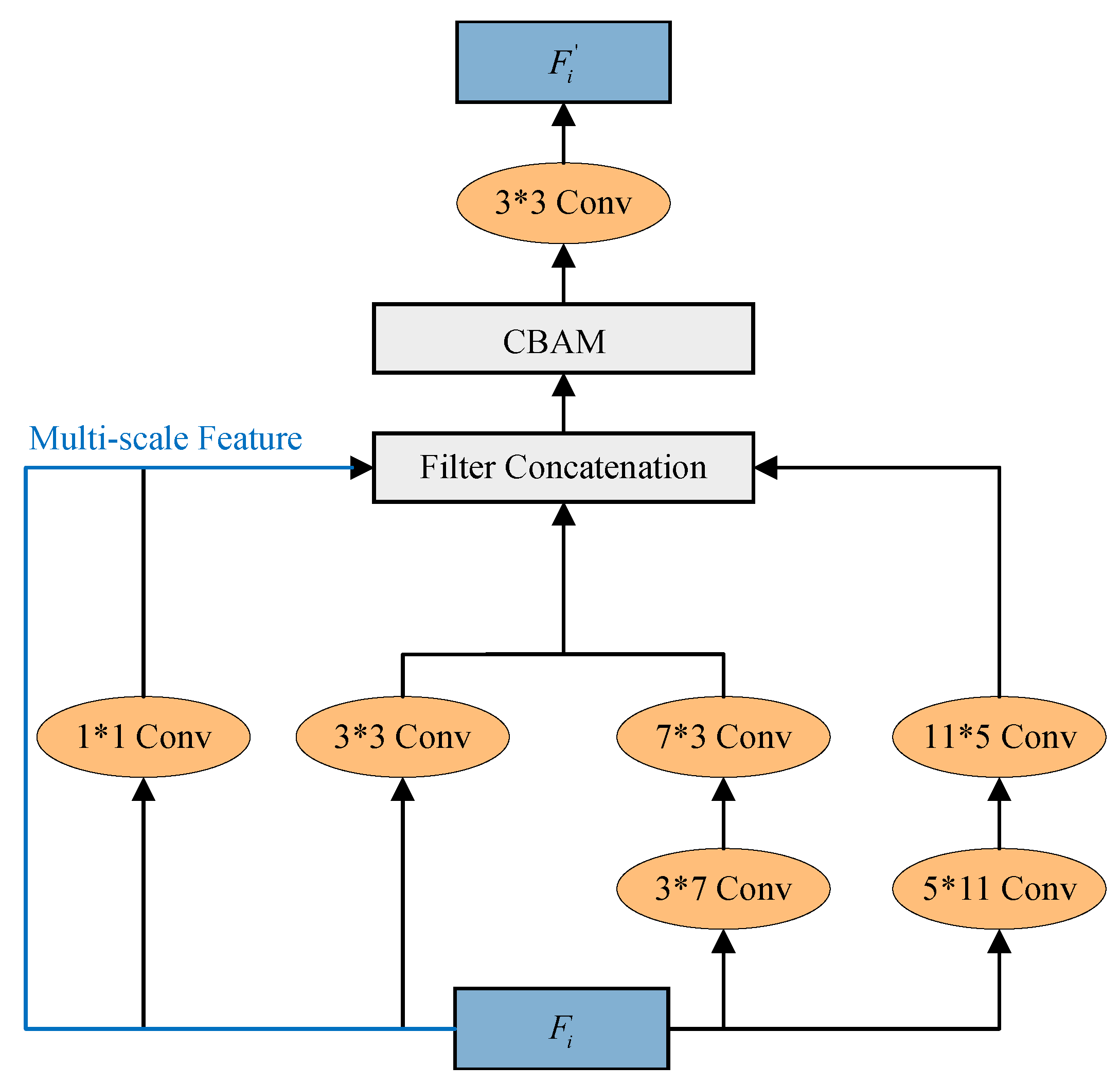
Magnetoelectric anomaly bodies can manifest at different locations and ranges within a geoelectric model. The encoding module generates multilevel feature information ( T i ) for magnetoelectric forward simulation data. During the upsampling process, the use of a single-size convolutional kernel may result in the loss of some feature information pertaining to multiple anomaly bodies. We employed convolutional kernels of different sizes to handle the hierarchical feature information, allowing each channel to focus more on specific details corresponding to the respective scale. This enhances the decoding process’s ability to recover anomaly positions and ranges. Additionally, smaller convolutional kernels reduce the complexity of parameters and computations without affecting the receptive field. Based on the convolution kernel and hierarchical features at different scales, we developed a multiscale adaptive decoding structure, whose structure is shown in Figure 4.
The decoder consists of four multiscale adaptive modules; each utilizes a multihead design. Each multiscale adaptive module (MSAM) consists of seven convolutional kernels of varying sizes and one convolutional block attention module (CBAM) [32]. The CBAM is a lightweight attention module that can conduct attention operations in both spatial and channel dimensions, thereby accentuating the significance of crucial feature information. Numerous studies have demonstrated consistent performance improvements by integrating CBAM into various models [33,34]. During the decoding process, the first MSAM receives the multilevel feature information ( T 4 ) generated by MiT-Block4 and uses it as the input tensor ( F 1 ), F 1 = H 32 × W 32 × 512. Using a 1 × 1 convolution, the input tensor is combined with channel information. To extract detailed features, a 3 × 3 convolution is applied. Convolutions of various sizes, including 3 × 7, 7 × 3, 5 × 11, and 11 × 5, are utilized to capture features at different scales along both the horizontal and vertical directions. The output tensors retain the same height (H) and width (W) dimensions as the input tensor but with a reduced channel size of 1/4. By incorporating tensors obtained from various convolutions and establishing residual connections with the input, ( F 1 ) integrates multiscale information. In the case of magnetoelectric results within distinct geoelectric models, different aspects are emphasized by utilizing the spatial and channel attention mechanism of CBAM. Subsequently, a 3 × 3 convolution is performed to obtain tensor F 1 . After upsampling, the H and W of F 1 increase by a factor of 2, while the channel count decreases from 512 to 320, resulting in tensor F 2 , F 2 = H 16 × W 16 × 320. The above process can be represented by Equation (3). By repeating this process, we obtain F 3 = H 8 × W 8 × 128 and F 4 = H 4 × W 4 × 64. Finally, F 4 maintains the same number of channels; after upsampling, the size becomes H 2 × W 2 × 64. Then, through output convolution and reducing the number of channels, the output size of H × W × 1 is obtained.
F i = MSAM ( F i ) , i ( 1 , 2 , 3 , 4 ) F j + 1 = Upsample ( F j ) , j ( 1 , 2 , 3 , 4 )
where MSAM() denotes the process of the input tensor F i being processed by MSAM to obtain F i , and Upsample () denotes the process of upsampling.

2.3. Network Training

In this study, following the classification method of Reitermanova training network [35], the 70,000 groups of data in the sample database were randomly divided in a ratio of 8:1:1: 56,000 groups in the training set, 7000 groups in the validation set, and 7000 groups in the test set were obtained.
The input data for network training are continuously downsampled in patch embedding and merging, and after the last encoding module, the size of the obtained data is 1/32 that of the original size. If the sample data are directly input into the forward network, the semantic information is seriously lost after four downsamplings. To avoid this situation, we interpolated the 32 × 128 sample data into the 256 × 1024. The encoder continuously acquires the original feature information through four MiT modules and gradually recovers to the output size of the forward result via transpose convolution and upsampling through four multiscale adaptive modules.
The anomalous body model has apparent resistivity values between 10 2 and 10 4 Ω m [36]. Sample data with too large a range increase the training time of the network and may make it difficult to converge, while normalized data have better performance in network training [37]. Therefore, normalizing the sample data before training reduces the stress of training while obtaining a better-performing network model.
In this study, we adopted the idea of maximum–minimum normalization: R h o is obtained by taking the logarithm of the resistivity and apparent resistivity data according to Equation (4) with a base of 10, at which time the data range is reduced to between −2 and 4. The maximum and minimum values of each data are counted separately, and the geoelectric model data, apparent resistivity data, and phase data are normalized according to Equations (5)–(7), respectively. When the network training is completed, reflective injection is executed to reduce the data to the original size.
R h o = log 10 R h o
R H O = R h o 1 Min 1 Max 1 Min 1
A R H O = R h o 2 Min 2 Max 2 Min 2
P H S = P h s Min 3 Max 3 Min 3
where R h o 1 is the resistivity data of the log10-processed geoelectric model, R h o 2 is the log10-processed apparent resistivity data, Phs is the phase data, and Max i and Min i (i = 1, 2, 3) denote the maximum and minimum values corresponding to each of the resistivity data, apparent resistivity data, and phase data, respectively. RHO denotes normalized geoelectric model resistivity data, ARHO denotes normalized apparent resistivity data, and PHS denotes normalized phase data.
The speed and performance of network convergence are influenced by the optimizer and loss function. For the MT-MitNet forward network model, the Adam [38] adaptive learning rate optimization algorithm is used for training, and the initial learning rate is 0.01. Forward and inversion MT modeling has high requirements for the accuracy of numerical simulations. The SmoothL1Loss loss function performs better for model convergence, anomalous body handling, and gradient explosion prevention, whereas the mean square error loss function creates the problem of gradient explosion at outlier points. Therefore, the SmoothL1Loss loss function was used in this study, which is calculated as follows:
S m o o t h L 1 L o s s ( X , Y ) = 1 N i = 0 N 0.5 ( X i Y i ) 2 , X i Y i < 1 X i Y i 0.5 , X i Y i 1
where X is the output of the MT-MitNet forward network, Y is the result of the conventional algorithm, and N is the number of samples. |X − Y| indicates the difference between them. When |X − Y| is less than 1, the squared error is used; otherwise, the linear error is used.
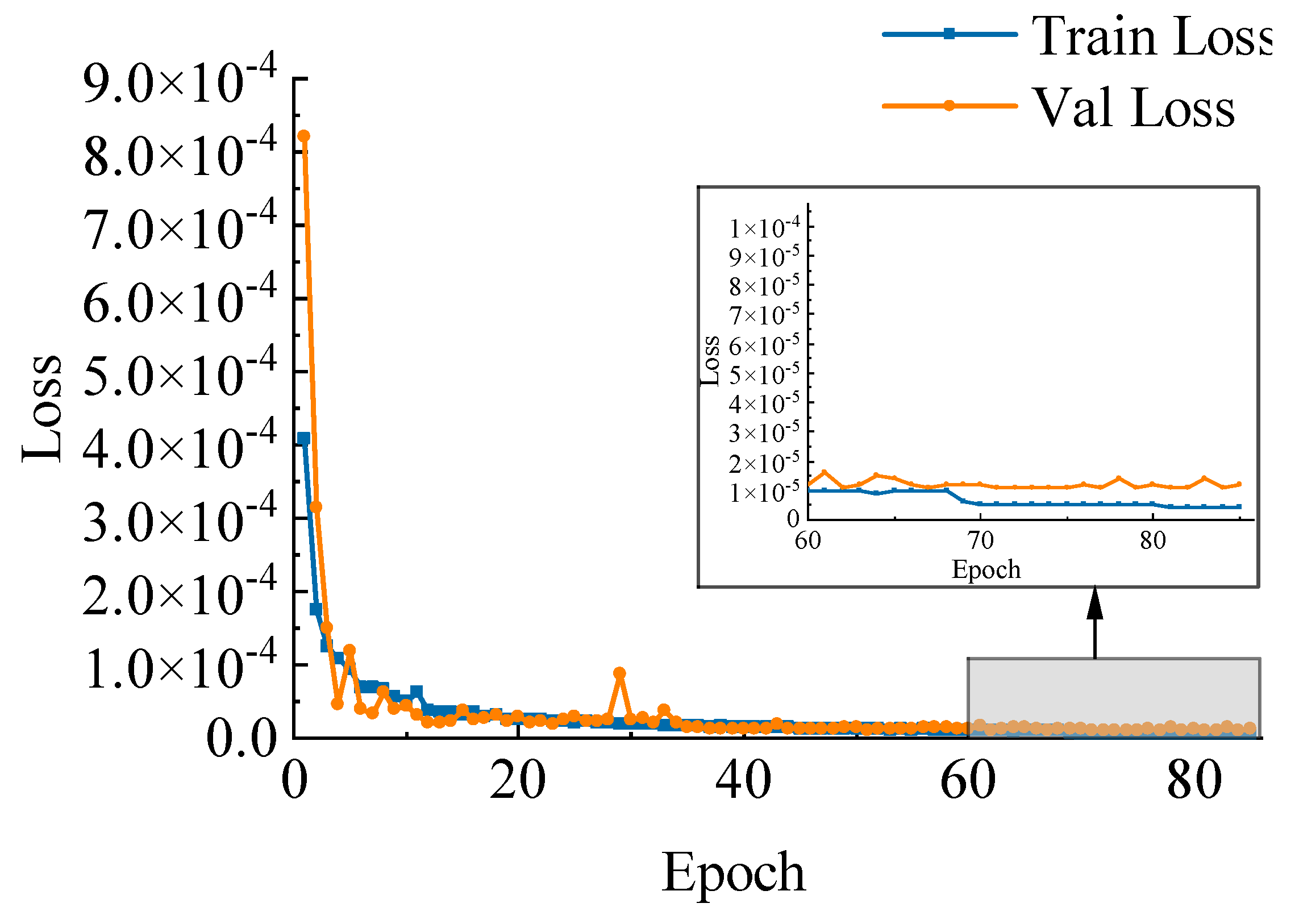
The experiments were conducted on an NVIDIA GeForce RTX 3090 GPU with 24 G VRAM. The training dataset consisted of 56,000 samples, and the validation and test datasets each contain 7000 samples. For the experiments, we employed the Adam optimizer with an initial learning rate of 0.01. The learning rate was reduced to 1/5 of its original value if the cumulative loss did not decrease for three consecutive epochs. The batch size was set to 2, and the training was performed for 100 epochs. The training was stopped when the validation loss remained within a small range of variation. The MT-MitNet forward network reduced the loss value to 5.0 × 10 5 in the first 10 rounds, stabilizing after 70 epochs. When the training epoch reached 80, the model loss value dropped to 4 × 10 6 , the learning rate was 4.0 × 10 7 , and the validation loss curve oscillated and stabilized in the range of 1.1 × 10 5 to 1.4 × 10 5 , the network model training was finished. The training and validation curves are shown in Figure 5.

3. Experiments

3.1. MT-MitNet Forward Network Model Replaces the Forward Computation Module of Occam Inversion Program

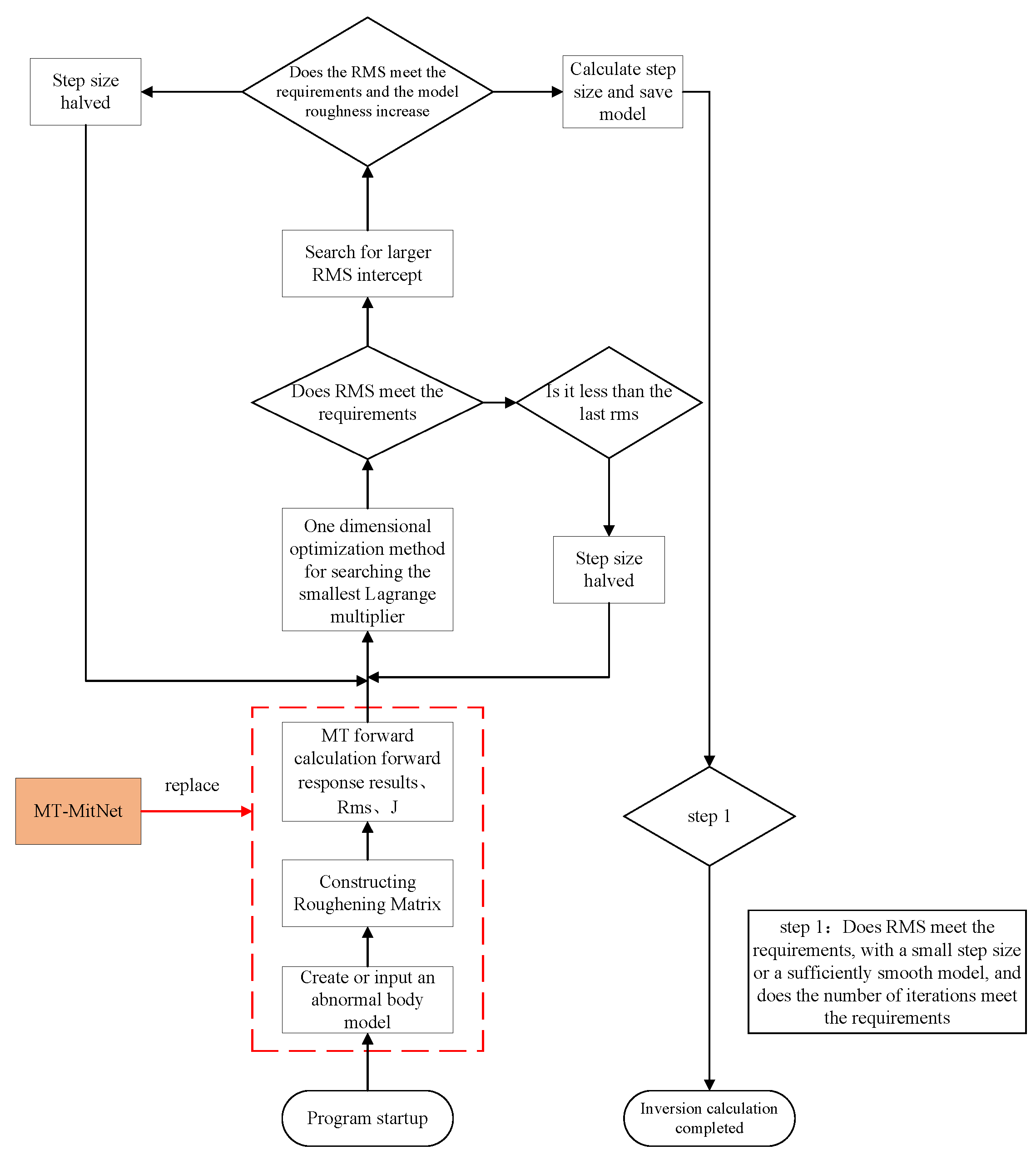
The traditional Occam inversion program is developed in Fortran language, and the inversion starts with the creation or input of the forward response data and the geoelectric model. The inversion algorithm performs several forward runs to find the best iterations for the purpose of reducing the fitting error, but the forward computation is less efficient. Using the trained MT-MitNet network can effectively reduce the forward computation time. However, the Occam inversion program runs in the Fortran development environment, and the forward network model is generated in the Python (PyTorch) environment, both of which cannot be directly accessed and used. In order for the inversion program to successfully use the results predicted by the forward network when calculating the forward response, we wrote the forward network model as a dynamic link library that the inversion program can call. The dynamic link library includes methods for loading and using the MT-MitNet model, data transfer between the Occam program and the MT-MitNet model, and data format conversion. PyTorch [39] provides methods to migrate between different environments; in order to enable the Occam inversion program (Fortran) to call the MT-MitNet model for the forward computation, the steps are as follows: (1) convert MT-MitNet from a PyTorch model to a TorchScript model by utilizing TorchScript; (2) develop a dynamic link library for C++ model calling based on the PyTorch C++ API library (LibTorch), named ForwardScript, which can load the TorchScript model and compute the forward response based on the input model, and outputs it; (3) introduce ForwardScript into the Occam inversion main program (Fortran), replacing the original forward function in the Occam program and calling the ForwardScript deep learning forward dynamic link library instead. The implementation occurs in the form of a dynamic library, so that the Occam inversion program developed by the Fortran program calls the model loading function in the library function when the inversion is executed, calls the forward function in the dynamic link library when the Occam inversion program calculates the forward, and receives the predicted forward result returned by the dynamic library, finally allowing the forward network model to be successfully deployed in the inversion program to complete the replacement of the forward calculation. A simplified flow of the MT-MitNet network model replacing the forward computation module of the Occam inversion program is shown in Figure 6.
The simplified process of MT-MitNet Occam inversion is as follows: the anomaly model and the forward response data are input into the network, and the data are reflected and combined into an array of forward responses at the end of the network computation and passed into the Occam inversion program. The inversion algorithm itself judges the computation process based on the fit difference and model roughness. If the inversion result does not reach the requirement of the end of the algorithm, the step length is reduced and the search for the optimal Lagrange multiplier continues. The computation finishes when the fit difference of the inversion result meets the fixed value or the model is smooth enough. We evaluated the optimal convergence of the model using the fit difference, which is expressed as Rms.
In this study, we deployed the inversion-oriented deep learning forward network model to realize the loading and use of the forward computational model of the replaced Occam inversion program in C++ development environment, and we used the well-trained MT-MitNet to achieve fast and accurate forward computation in order to improve the efficiency of forward computation in inversion.

3.2. Experimental Analysis of the Inversion of MT-MitNet Replacement Forward Calculation

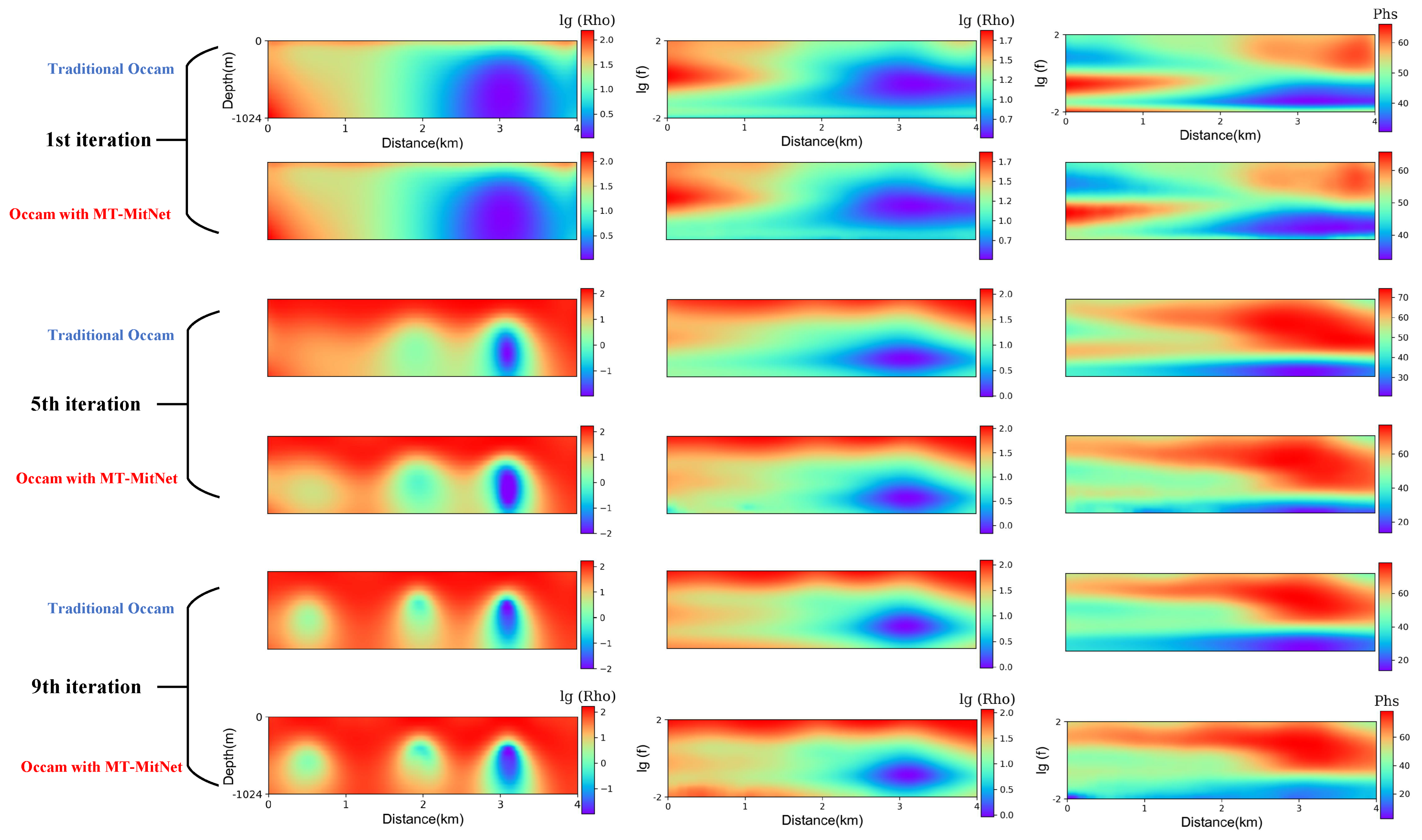
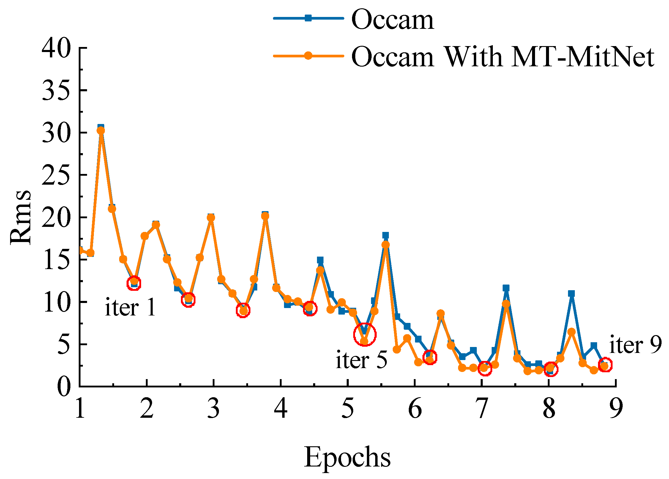
To evaluate the effectiveness of the MT-MitNet forward network in MT inversion applications, we randomly selected a geoelectric model with three anomalies. The model has a background resistivity of 100 Ω m and anomaly resistivity values of 3.16 Ω m, 1 Ω m, and 0.03 Ω m, respectively, from left to right, as shown in Figure 7. Firstly, the MT forward calculation is performed on the geoelectric model to obtain the forward response result. Then, the forward results were combined with the geoelectric model to form the observation data, which were further normalized and input into the Occam inversion program. Both the traditional Occam inversion method and the replacement of Occam’s forward modeling calculation process with MT-MitNet were used separately for computation. The iteration process stopped when the model reache a convergence point (reaches the target fitting difference), as shown in Figure 8.
The Occam inversion computed by MT-MitNet replacement forward and the traditional Occam inversion both converged and performed well after nine iterations, with Rms values of 1.805 and 1.88, respectively. Based on the iterative process and results, it could be observed that each round of the inversion iteration showed high correspondence between the model based on the MT-MitNet replacement forward computation and the traditional inversion method. The former also simulated the anomaly model, apparent resistivity, and phase with a high degree of similarity. Nine rounds of iterations of the model fit difference decline curve are shown in Figure 9. The algorithm is computed several times during each iteration to find the minimum fitting error in this round. Figure 9 marks the end position of each iteration with dashed red circles, corresponding to the results of rounds 1, 5, and 9 in Figure 8.
The anomalous body model was computed by stopping at nine iterations.The traditional Occam inversion method computed the forward response in about 2808.6 s, while the MT-MitNet achieved this task in about 4.3 s, indicating a remarkable increase in computational efficiency. After iterative computations, both methods accurately represented the size and location of the anomalous body.
In order to compare the accuracy difference between the inversion results of the forward response calculated by the deep learning network and the traditional inversion results, we generated images of the data results using Python 3.7, and according to the characteristics of the images, three different error statistics criteria were adopted in this study to evaluate the inversion results, the apparent resistivity results, and the phase results. The three methods were the average Euclidean distance error statistics, the histogram error statistics, and the average peak signal-to-noise ratio (Peak S/N) error statistics [40]. The computation equations are given in Equations (9)–(11).
Err avg = i = 1 W j = 1 H L i , j K i , j W × H
where W and H represent the width and height of the image, respectively; and L i , j and K i , j denote the results of the traditional Occam inversion and the results of the MT-MitNet computation at point ( i , j ) , respectively.
Err hist = 1 P i = 1 P ( 1 P i R i Max ( P i , R i ) ) , P i R i 1 , P i = R i
where P is the length of the image histogram, and P i and R i are the values of the forward results saved by the traditional Occam inversion and the results calculated by the MT-MitNet at the point i on the histogram, respectively.
Err Peak = 20 · log 10 MAX I i = 1 W j = 1 H L i , j K i , j 2 W × H
where MAX I is the maximum pixel value of the image; the maximum value after normalization of the data in this study was 1, so MAX I was taken as 1. W and H represent the width and height of the image, respectively; L i , j and K i , j denote the results of traditional Occam inversion results and MT-MitNet computation results at point of ( i , j ) , respectively.
The triple anomaly model undergoes nine iterations in the Occam inversion method using the MT-MitNet replacement forward computation, and its inversion results and forward response are shown in Table 1, along with the inversion results and forward response error of the traditional Occam inversion method.
From Table 1, it is evident that the computed results for the anomalous body exhibited an accuracy of more than 95% as indicated by the Euclidean distance, which represents high precision. A Peak S/N result above 30 dB signifies a high degree of similarity between any two compared images. Such a degree of similarity is reflected in the inversion and forward results of the model that are highly in agreement. The evident accuracy indicates that the Occam inversion method with deep learning replacing forward calculation can potentially simulate the traditional Occam forward iterative process. Furthermore, MT-MitNet computed forward results with high accuracy, meeting the requirements of inversion accuracy. The MT-MitNet inversion achieved relatively ideal results when dealing with multiple, complex anomalous bodies.
To test the effectiveness of the MT-MitNet method more comprehensively, 1000 groups of data were randomly selected from the 7000 groups of test sets in the forwarding sample dataset. We evaluated these models under the same experimental conditions as previously described. The model forward responses of these 1000 data groups were combined as observed data, and inversion was performed using the traditional Occam inversion method and the method based on deep learning replacement forward computation, separately. Table 2 gives the average forward elapsed time of the inversion computation for the 1000 data groups for both methods, and Table 3 gives the average error of the forward response computation part of the inversion computation for the 1000 test set data using the MT-MitNet method under the three error evaluation approaches.
The results of the test set experiments showed that the inversion-oriented deep-learning-accelerated forward computation of the Occam inversion method is highly similar to the traditional Occam inversion method in terms of inversion results and forward responses. The average MT-MitNet forward time is about 1/653 that of the traditional Occam forward average time, and the forward efficiency is greatly improved. The validation of the test data proved the effectiveness of the inversion-oriented deep learning forwarding method.
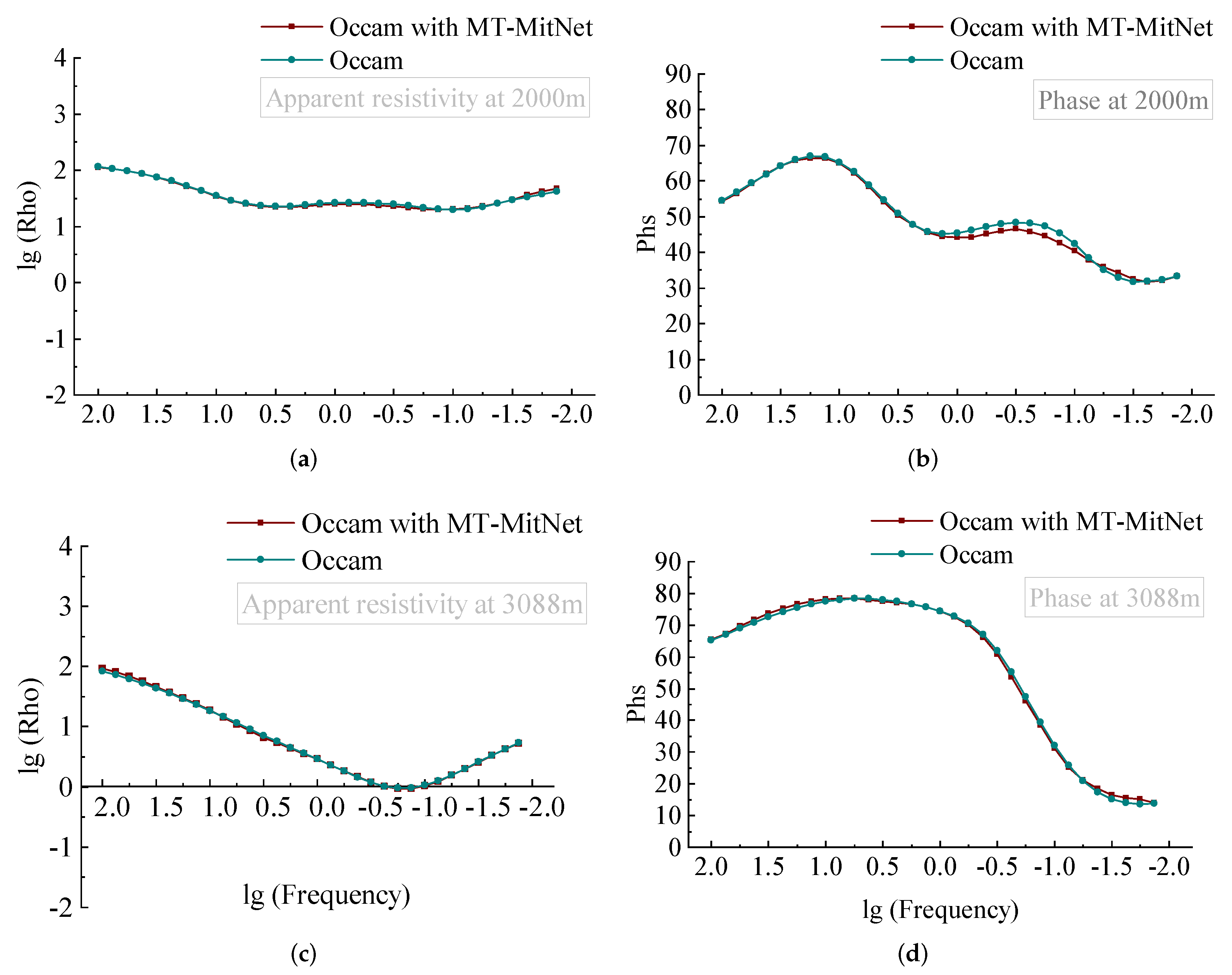
To further compare the differences between the MT-MitNet replacement forward computation results and the traditional inversion results, the computation results located at 2000 m and 3088 m of the geoelectric model were extracted for comparison and analysis, as shown in Figure 10 and Figure 11.
The results demonstrate that replacing forward computation with inversion-oriented deep learning yields commendable outcomes. MT-MitNet provides computed values for phase and apparent resistivity that are essentially in agreement with those obtained from traditional methods. Moreover, MT-MitNet accurately identifies the model’s subtle differences and responds appropriately, demonstrating its high accuracy. This finding establishes that this approach renders results with high precision in less time.

4. Conclusions

The proposed deep learning network can precisely simulate the magnetotelluric forward modeling and improve the forward speed. This study applied deep learning to the forward response calculation in MT inversion. By using the forward data generated by traditional inversion calculations, we established a crucial sample dataset for training a deep learning network. We proposed a forward network model named MT-MitNet, based on Mit-Transformer, which can globally model and obtain more abundant feature information and execute faster forward simulations with high accuracy. The experimental results demonstrated that MT-MitNet can accurately simulate the traditional forward method by replacing its traditional forward calculation process in inversion. It has precise forward results that fulfill the requirements of inversion accuracy, with an average resistivity accuracy of 98.4% and an average phase accuracy of 97.42%. MT-MitNet also shows a strong generalization ability in the complex multiple anomalous bodies model.

Author Contributions

Conceptualization, F.D. and J.H.; methodology, F.D. and J.H.; software, F.D. and X.W.; validation, F.D.; formal analysis, S.L., X.W., X.L. and B.Z.; investigation, X.W., S.L. and S.Y.; resources, X.W., B.Z., X.L. and S.L.; data curation, S.L., S.Y. and B.Z.; writing—original draft, F.D. and J.H.; writing—review and editing, F.D. and J.H.; visualization, X.W.; supervision, F.D.; project administration, B.Z., S.Y., X.L. and S.L. All authors have read and agreed to the published version of the manuscript.

Funding

This article was supported by a grant from the National Natural Science Foundation of China (41930112).

Data Availability Statement

Not applicable.

Conflicts of Interest

The authors declare no conflict of interest.

References

  1. Tikhonov, A.N. On determining electrical characteristics of the deep layers of the Earth’s crust. Dokl. Akad. Nauk. SSSR 1950, 73, 295–297. [Google Scholar]
  2. Cagniard, L. Basic theory of the magneto-telluric method of geophysical prospecting. Geophysics 1953, 18, 605–635. [Google Scholar] [CrossRef]
  3. Constable, S.C.; Parker, R.; Constable, C. A practical algorithm for generating smooth models from electromagnetic sounding data. Geophysics 1987, 52, 289–300. [Google Scholar] [CrossRef]
  4. De Groot Hedlin, C.; Constable, S. Occam’s inversion to generate smooth, two-dimensional models from magnetotelluric data. Geophysics 1990, 55, 1613–1624. [Google Scholar] [CrossRef] [Green Version]
  5. Smith, J.T.; Booker, J.R. Rapid inversion of two-and three-dimensional magnetotelluric data. J. Geophys. Res. Solid Earth 1991, 96, 3905–3922. [Google Scholar] [CrossRef]
  6. Newman, G.A.; Alumbaugh, D.L. Three-dimensional magnetotelluric inversion using non-linear conjugate gradients. Geophys. J. Int. 2000, 140, 410–424. [Google Scholar] [CrossRef] [Green Version]
  7. Rodi, W.; Mackie, R.L. Nonlinear conjugate gradients algorithm for 2-D magnetotelluric inversion. Geophysics 2001, 66, 174–187. [Google Scholar] [CrossRef]
  8. Pratt, R.G.; Shin, C.; Hick, G. Gauss—Newton and full Newton methods in frequency—Space seismic waveform inversion. Geophys. J. Int. 1998, 133, 341–362. [Google Scholar] [CrossRef]
  9. Loke, M.H.; Dahlin, T. A comparison of the Gauss—Newton and quasi-Newton methods in resistivity imaging inversion. J. Appl. Geophys. 2002, 49, 149–162. [Google Scholar] [CrossRef] [Green Version]
  10. Jones, A.G. On the equivalence of the “Niblett” and “Bostick” transformations in the magnetotelluric method. J. Geophys. 1983, 53, 72–73. [Google Scholar]
  11. Montahaei, M.; Oskooi, B. Magnetotelluric inversion for azimuthally anisotropic resistivities employing artificial neural networks. Acta Geophys. 2014, 62, 12–43. [Google Scholar] [CrossRef]
  12. Fang, J.; Zhou, H.; Li, Y.E.; Zhang, Q.; Wang, L.; Sun, P.; Zhang, J. Data-driven low-frequency signal recovery using deep-learning predictions in full-waveform inversion. Geophysics 2020, 85, A37–A43. [Google Scholar] [CrossRef]
  13. Moseley, B.; Markham, A.; Nissen-Meyer, T. Fast approximate simulation of seismic waves with deep learning. arXiv 2018, arXiv:1807.06873. [Google Scholar]
  14. Hansen, T.M.; Cordua, K.S. Efficient Monte Carlo sampling of inverse problems using a neural network-based forward—Applied to GPR crosshole traveltime inversion. Geophys. J. Int. 2017, 211, 1524–1533. [Google Scholar] [CrossRef]
  15. Li, S.; Liu, B.; Ren, Y.; Chen, Y.; Yang, S.; Wang, Y.; Jiang, P. Deep-learning inversion of seismic data. arXiv 2019, arXiv:1901.07733. [Google Scholar] [CrossRef] [Green Version]
  16. Puzyrev, V. Deep learning electromagnetic inversion with convolutional neural networks. Geophys. J. Int. 2019, 218, 817–832. [Google Scholar] [CrossRef] [Green Version]
  17. Puzyrev, V.; Swidinsky, A. Inversion of 1D frequency-and time-domain electromagnetic data with convolutional neural networks. Comput. Geosci. 2021, 149, 104681. [Google Scholar] [CrossRef]
  18. Liu, W.; Wang, H.; Xi, Z.; Zhang, R.; Huang, X. Physics-Driven Deep Learning Inversion with Application to Magnetotelluric. Remote Sens. 2022, 14, 3218. [Google Scholar] [CrossRef]
  19. Conway, D.; Alexander, B.; King, M.; Heinson, G.; Kee, Y. Inverting magnetotelluric responses in a three-dimensional earth using fast forward approximations based on artificial neural networks. Comput. Geosci. 2019, 127, 44–52. [Google Scholar] [CrossRef]
  20. Liu, B.; Guo, Q.; Li, S.; Liu, B.; Ren, Y.; Pang, Y.; Guo, X.; Liu, L.; Jiang, P. Deep learning inversion of electrical resistivity data. IEEE Trans. Geosci. Remote Sens. 2020, 58, 5715–5728. [Google Scholar] [CrossRef] [Green Version]
  21. Guo, R.; Li, M.; Fang, G.; Yang, F.; Xu, S.; Abubakar, A. Application of supervised descent method to transient electromagnetic data inversion. Geophysics 2019, 84, E225–E237. [Google Scholar] [CrossRef]
  22. Xie, E.; Wang, W.; Yu, Z.; Anandkumar, A.; Alvarez, J.M.; Luo, P. SegFormer: Simple and efficient design for semantic segmentation with transformers. Adv. Neural Inf. Process. Syst. 2021, 34, 12077–12090. [Google Scholar]
  23. Sharma, H.; Zhang, Q. Transient electromagnetic modeling using recurrent neural networks. In Proceedings of the IEEE MTT-S International Microwave Symposium Digest, Long Beach, CA, USA, 17 June 2005; pp. 1597–1600. [Google Scholar]
  24. Hochreiter, S.; Schmidhuber, J. Long short-term memory. Neural Comput. 1997, 9, 1735–1780. [Google Scholar] [CrossRef] [PubMed]
  25. Ovcharenko, O.; Kazei, V.; Kalita, M.; Peter, D.; Alkhalifah, T. Deep learning for low-frequency extrapolation from multioffset seismic dataDeep learning for low-frequency extrapolation. Geophysics 2019, 84, R989–R1001. [Google Scholar] [CrossRef] [Green Version]
  26. Lewis, W.; Vigh, D. Deep learning prior models from seismic images for full-waveform inversion. In Proceedings of the 2017 SEG International Exposition and Annual Meeting, Houston, TX, USA, 24–29 September 2017; OnePetro: Richardson, TX, USA, 2017. [Google Scholar]
  27. Mao, B.; Han, L.G.; Feng, Q.; Yin, Y.C. Subsurface velocity inversion from deep learning-based data assimilation. J. Appl. Geophys. 2019, 167, 172–179. [Google Scholar] [CrossRef]
  28. Long, J.; Shelhamer, E.; Darrell, T. Fully convolutional networks for semantic segmentation. In Proceedings of the IEEE Conference on Computer Vision and Pattern Recognition, Boston, MA, USA, 7–12 June 2015; pp. 3431–3440. [Google Scholar]
  29. Vaswani, A.; Shazeer, N.; Parmar, N.; Uszkoreit, J.; Jones, L.; Gomez, A.N.; Kaiser, L.; Polosukhin, I. Attention is all you need. Adv. Neural Inf. Process. Syst. 2017, 30. [Google Scholar] [CrossRef]
  30. Dosovitskiy, A.; Beyer, L.; Kolesnikov, A.; Weissenborn, D.; Zhai, X.; Unterthiner, T.; Dehghani, M.; Minderer, M.; Heigold, G.; Gelly, S.; et al. An image is worth 16 × 16 words: Transformers for image recognition at scale. arXiv 2020, arXiv:2010.11929. [Google Scholar]
  31. Deng, F.; Yu, S.; Wang, X.; Guo, Z. Accelerating magnetotelluric forward modeling with deep learning: Conv-BiLSTM and D-LinkNet. Geophysics 2023, 88, E69–E77. [Google Scholar] [CrossRef]
  32. Woo, S.; Park, J.; Lee, J.Y.; Kweon, I.S. Cbam: Convolutional block attention module. In Proceedings of the European Conference on Computer Vision (ECCV), Munich, Germany, 8–14 September 2018; pp. 3–19. [Google Scholar]
  33. Wang, W.; Tan, X.; Zhang, P.; Wang, X. A CBAM based multiscale transformer fusion approach for remote sensing image change detection. IEEE J. Sel. Top. Appl. Earth Obs. Remote Sens. 2022, 15, 6817–6825. [Google Scholar] [CrossRef]
  34. Fu, H.; Song, G.; Wang, Y. Improved YOLOv4 marine target detection combined with CBAM. Symmetry 2021, 13, 623. [Google Scholar] [CrossRef]
  35. Reitermanova, Z. Data Splitting. In WDS’10 Proceedings of Contributed Papers; Part I; Matfyzpress: Prague, Czechia, 2010; pp. 31–36. [Google Scholar]
  36. Warner, R.W. Earth Resistivity as Affected by the Presence of Underground Water. Trans. Kans. Acad. Sci. 1935, 38, 235–241. [Google Scholar] [CrossRef]
  37. El-Qady, G.; Ushijima, K. Inversion of DC resistivity data using neural networks. Geophys. Prospect. 2001, 49, 417–430. [Google Scholar] [CrossRef]
  38. Kingma, D.P.; Ba, J. Adam: A method for stochastic optimization. arXiv 2014, arXiv:1412.6980. [Google Scholar]
  39. Paszke, A.; Gross, S.; Massa, F.; Lerer, A.; Bradbury, J.P. An imperative style, high-performance deep learning library. Adv. Neural Inf. Process. Syst. 2019, 32, 8026–8037. [Google Scholar]
  40. Li, Q.; Zhang, W.; Li, M.; Niu, J.; Wu, Q.J. Automatic detection of ship targets based on wavelet transform for HF surface wavelet radar. IEEE Geosci. Remote Sens. Lett. 2017, 14, 714–718. [Google Scholar] [CrossRef]
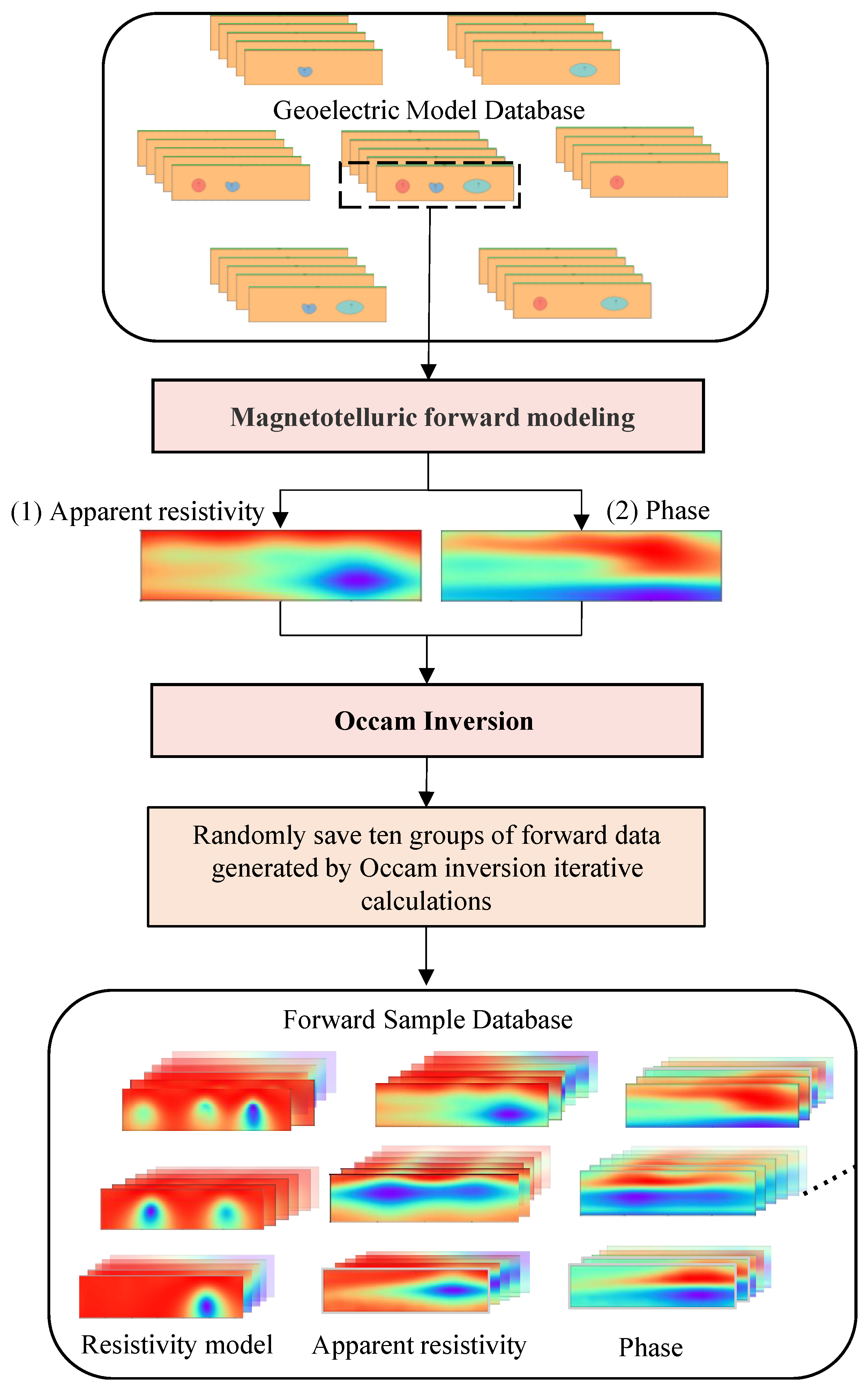
Figure 1. Sample data production process.
Remotesensing 15 03667 g001
Figure 2. MT-MitNet forward network model structure.
Remotesensing 15 03667 g002
Figure 3. MixTransformer Block (values of n for the 4 MiT-Blocks are 3, 8, 27, and 3, respectively).
Remotesensing 15 03667 g003
Figure 4. Multiscale adaptive module decoding structure.
Remotesensing 15 03667 g004
Figure 5. Training and validation curves of MT-MitNet.
Remotesensing 15 03667 g005
Figure 6. Simplified MT-MitNet Occam inversion process.
Remotesensing 15 03667 g006
Figure 7. The three anomaly models and their MT forward response results, from left to right, are anomaly geoelectric model, apparent resistivity results, and phase results.
Remotesensing 15 03667 g007
Figure 8. The results of the 1st iteration, 5th iteration, and 9th iteration of the traditional Occam inversion and MT-MitNet replacement forward computations, from left to right, are resistivity results, apparent resistivity results, and phase results, respectively.
Remotesensing 15 03667 g008
Figure 9. A plot of the Rms from the optimized model searched for at each iteration of the inversion process, as calculated by the traditional Occam inversion (blue) and the MT-MitNet replacement forward calculation (orange). The inversion algorithm invokes the forward computation several times during the inversion process to find the optimal model in an optimization-seeking iteration. The multiple points in the figure represent the optimized models found by the Occam inversion algorithm in each iteration.
Remotesensing 15 03667 g009
Figure 10. Comparison of inversion results: from left to right, resistivity results, apparent resistivity results, and phase results, respectively.
Remotesensing 15 03667 g010
Figure 11. Comparison of the forward results of the observation sites: (a) Apparent resistivity comparison curve at 2000 m; (b) Phase comparison curve at 2000 m; (c) Apparent resistivity comparison curve at 3088 m; (d) Phase comparison curve at 3088 m.
Remotesensing 15 03667 g011
Table 1. Error of inversion results of three-anomalies model.
Average Euclidean Distance (%)Histogram (%)Peak S/N (dB)
Resistivity4.2922.6031.55
Apparent Resistivity1.6019.2733.36
Phase2.5821.9932.81
Table 2. Forward computation of the average schedule.
Average Time Taken for Forward Computation (s)
Traditional Occam2619.1
MT-MitNet Occam4.0
Table 3. Test set data results’ error.
Average Euclidean Distance (%)Histogram (%)Peak S/N (dB)
Resistivity4.2522.6431.60
Apparent Resistivity1.6419.3233.34
Phase2.4321.9532.89
Disclaimer/Publisher’s Note: The statements, opinions and data contained in all publications are solely those of the individual author(s) and contributor(s) and not of MDPI and/or the editor(s). MDPI and/or the editor(s) disclaim responsibility for any injury to people or property resulting from any ideas, methods, instructions or products referred to in the content.