Novel Method for Determining the Height of the Stable Boundary Layer under Low-Level Jet by Judging the Shape of the Wind Velocity Variance Profile

Abstract

The height of the stable boundary layer is a key parameter in atmospheric transmission and diffusion, air quality, emergency response, wind energy, and numerical weather prediction models. Existing methods mainly determine the stable boundary layer height via a threshold or minimum value of the wind speed variance under a low-level jet. Based on multi-meteorological element data from a meteorological gradient observation tower, this paper revealed the limitations of existing methods from the perspective of dynamic and thermal effects. In this paper, it is demonstrated that there were four types of shapes of the wind speed variance profile under the low-level jet and a method for using the shape of the variance profile to retrieve the height of the stable boundary layer was proposed. This method distinguished different types of wind speed variance profiles and solved the problems of the misjudgment and omissions (about 34%) present in existing methods. Our experiment showed that the average absolute error of the proposed method was less than 18 m and the average relative error was less than 9%. The results showed that the proposed inversion method was extended to all kinds of wind field detection equipment for inversion of the stable boundary layer height and has very high universality.

1. Introduction

The height of the atmospheric boundary layer is an important parameter to determine the characteristics of the atmospheric boundary layer, reflecting physical processes such as turbulent mixing and convection development in the boundary layer, which affect the vertical distribution of the heat, water vapor, aerosols, and other substances and energy [1,2,3]. The nighttime stable boundary layer height is a key parameter in atmospheric transmission and diffusion, air quality, emergency response, wind energy, and numerical weather prediction models [4,5,6]. It is of great practical value to study the inversion methods and variation laws of the stable boundary layer height.

As an unconventional observation variable, the stable boundary layer height cannot be directly measured but instead is mainly determined by analyzing the variation characteristics of atmospheric elements in the vertical direction. The important trade-off in studying the height of the stable boundary layer is to obtain the statistics of fluctuations over time, such as variance [7,8]. Therefore, the key is to obtain reliable high resolution profile measurements. Wind lidar can measure the vertical distribution of the atmospheric wind field, with very high time resolution and accuracy [9]. The usual method is to consider a low-level jet to retrieve the height of the stable boundary layer [10,11,12,13,14,15]. Vicker et al. and Lemone et al. mainly reduced the wind speed variance to a certain proportion of the maximum value near the ground as the stable boundary layer height [16,17]. This ratio is usually 0.05 to 0.1. Schween et al. found that a 25% threshold change will cause a 7% deviation of the boundary layer height, and the threshold selection is also different for different weather conditions [18]. Therefore, it is still difficult to determine the threshold at the current stage to determine the boundary layer height from the wind speed variance. In addition, other researchers mainly obtain the stable boundary layer height based on the minimum position of the wind speed variance under a low-level jet [10,11,12,19]. Previous studies have shown that there are many causes of low-level jets, including synoptic scale baroclinicity related to weather patterns, baroclinicity related to slope topography, frontal advection acceleration, airflow branches around the same ground obstacles, waveguides and convergence, sea and land winds, valley winds, and inertial oscillations [20]. In some cases, more than one of the above factors will affect the formation of the jet stream at the same time. Therefore, there are many types of low-level jet streams with different characteristics [20]. This means that the height determined by the threshold or minimum value of the wind speed variance under the low-level jet is not necessarily the stable boundary layer height.

Meteorological gradient observation towers are a reliable data source for studying the stable boundary layer height. They can provide high-resolution profile measurements of multiple meteorological elements, which can be used to study the internal dynamic characteristics of the boundary layer. Based on the problems mentioned above, this paper took advantage of the direct and continuous measurements of multiple meteorological elements located at the 350 m high Shenzhen Meteorological Gradient Observation Tower and obtains the nighttime boundary layer height below 350 m based on an inversion method that uses the Richardson number from the perspective of dynamic and thermal effects. It is used as the evaluation standard to reveal the characteristics of wind speed variance under a low-level jet stream and then to verify the accuracy of retrieving the stable boundary layer height using the wind speed variance threshold or minimum method.

2. Methods

Whether there is turbulent motion is the essential difference between the atmospheric boundary layer and the free atmosphere [20]. Turbulence and nonturbulence can be distinguished according to the Richardson number, as shown in Equation (1):

$$Ri=\frac{g}{\theta }\frac{\mathsf{\Delta }\theta /\mathsf{\Delta }z}{{\left(\mathsf{\Delta }U/\mathsf{\Delta }z\right)}^2}$$

(1)

where g is the acceleration of gravity, θ is the virtual potential temperature, U is the wind speed, and z is the height [20].

The Richardson number method integrates dynamic and thermal effects, and considers physical processes comprehensively, which is widely used in the analysis of stable boundary layer [21,22,23,24]. Vogelezang et al. divided the critical values of the Richardson number into different categories based on different stratification conditions, with the critical value of weak neutral stability stratification being 0.23–0 32 and the strong stability condition layer divided into 0.16–0.22 [22]. Nieuwstadt set Ri = 0.2, and obtained the height of the stable boundary layer by solving the equations of motion [25]. Overall, existing theoretical and experimental studies have shown that when the Richardson number is greater than the critical value (~0.25), it can be considered that there is a stable boundary layer [20]. There is a transition between the height of the stable boundary layer and the atmospheric residual layer. In practical applications, the lowest height at which the Richardson number exceeds the critical value is often regarded as the height of the stable boundary layer, thus excluding the residual layer. Therefore, the boundary layer height in this study refers to the lowest height where the Richardson number reaches 0.25, which is the same as used by Seidel [23,24].

The Shenzhen meteorological gradient observation tower is located near a reservoir, approximately 1 km from the nearest building and approximately 10 km from the coastline. Due to its excellent geographical location (113.897°E, 22.649°N) with no obstructions around it, the monitored data are highly representative. It has a total of 13 conventional meteorological element observation automatic stations (measuring the wind speed, temperature, humidity, and atmospheric pressure), which are distributed on platforms at altitudes of 10, 20, 40, 50, 80, 100, 150, 160, 200, 250, 300, 320, and 350 m, and sample with a temporal resolution of 10 s. With such data, and employing Equation (1), the Richardson number can be calculated, and then the stable boundary layer height can be obtained. Based on the Richardson number, we can obtain the characteristics of wind speed variance under low-level jets as well as the law of retrieving stable boundary layer height from wind speed variance. The purpose is to establish a new stable boundary layer height algorithm suitable for all wind field monitoring equipment.

Figure 1 shows the spatial and temporal distribution of the horizontal wind speed, virtual potential temperature, wind speed variance, and Richardson number monitored by the Shenzhen Meteorological Gradient Observation Tower on 2 August 2022. Due to differences in the height, range, wind speed intensity, and horizontal and vertical shear of low-level jet streams, there is currently no unified standard definition for low-level jet streams. Bonner’s standards are ΔV = Vmax − Vmin ≥ 2.6 m/s, where Vmax is the maximum wind speed of the profile and Vmin is the minimum wind speed immediately above Vmax [26]. Referring to this standard, in this article, we define a low-level jet stream where the maximum wind speed occurs below a height of 1000 m, with Vmax ≥ 5 m/s and ΔV ≥ 2.6 m/s. It can be seen from Figure 1a that there is a low-level jet for some periods during the day, and there is also an obvious inversion layer, seen in Figure 1b, in the virtual potential temperature at the corresponding time. From Figure 1a, it can also be seen that the peak height of the low-level jet stream continuously increases over time. After 23:00, the height of the low-level jet surpassed 350 m, exceeding the monitoring range of the gradient observation tower. In order to clearly see the changes in the various meteorological elements under the low-level jet, only data with a peak height of 350 m or less are displayed. For the horizontal wind speed (W) in Figure 1c, it is decomposed into Wu (along the east–west direction) and Wv (along the north–south direction) components, using 10 min intervals (thus, based on a time resolution of 10 s, there are 60 data groups). Using a sliding method (e.g., such as using data from groups 1 to 60 and then from groups 2 to 61, etc.), the wind speed variances in these two directions, δ_u and δ_v, with a time resolution of 10 s, are calculated separately. We calculate the variance of the horizontal wind speed as δ = δ_u + δ_v. It can be clearly seen from the variance profile in Figure 1c that when a low-level jet is extant, the variance profile has a relatively large value near the ground, while there is a significant decrease in the upper air. The Richardson number distribution in Figure 1d shows that there is an obvious large Richardson number at the time and location of the low-level jet. This demonstrates that there is a laminar flow layer, that is, a stable boundary layer.

The horizontal wind speed, wind speed variance, virtual potential temperature, and Richardson number at different times are extracted, as shown in Figure 2. It can be seen from Figure 2a that there are low-level jets at these four times, and the peak wind speed is greater than 5 m/s. It can be seen from Figure 2b that there are four types of variance profile shape, of which type B and D have previously been discussed in the literature [10,11,12,19], and we find that at the height of the maximum wind speed, the variance has a minimum value. For types A and C, the variance of the corresponding position of the peak is a maximum, and these profile types have not been found in previous studies. From the temperature and Richardson number shown in Figure 2c and d, respectively, it can be seen that in the case of type A, there is no stable boundary layer, while in type C, there is a stable boundary layer. Based on the data from August 2022 (sample size = 53,816), the frequency and proportion of these four types were calculated, as shown in

Table 1. Frequency and proportion of the four types of wind speed variance profiles based on the data from August 2022.

Type	A	B	C	D
Frequency	16,840	16,521	1460	18,995
Proportion	31.3%	30.7%	2.7%	35.3%

. From Table 1, we can see that type B and type D have the highest frequency, and their proportions can reach 66%. For type A, the proportion is 31.3%, which corresponds to the 31.3% misjudgment rate seen in previous studies that used low-level jets to extract the stable boundary layer height. For type C, the proportion is 2.7%, which corresponds to the missed judgment rate of 2.7% in previous studies.

Therefore, in this paper, we propose a method to determine the stable boundary layer height based on the shapes of these four types of variance profiles. When a low-level jet appears, the variance profile is calculated to determine whether it belongs to type B, C, or D, so as to determine the position of the maximum wind speed as the stable boundary layer height. Figure 3 shows the correlation between the stable boundary layer height obtained using the Richardson number method and that retrieved from the variance profile shape based on the data from August 2022. Due to the low spatial resolution of the gradient observation tower data, the data points in the figure appear to be relatively few, but in fact, each point represents a particularly large sample size (~36,000 data points).

Table 2. Error of the stable boundary layer height obtained by the Richardson number method and that retrieved from variance profile shape.

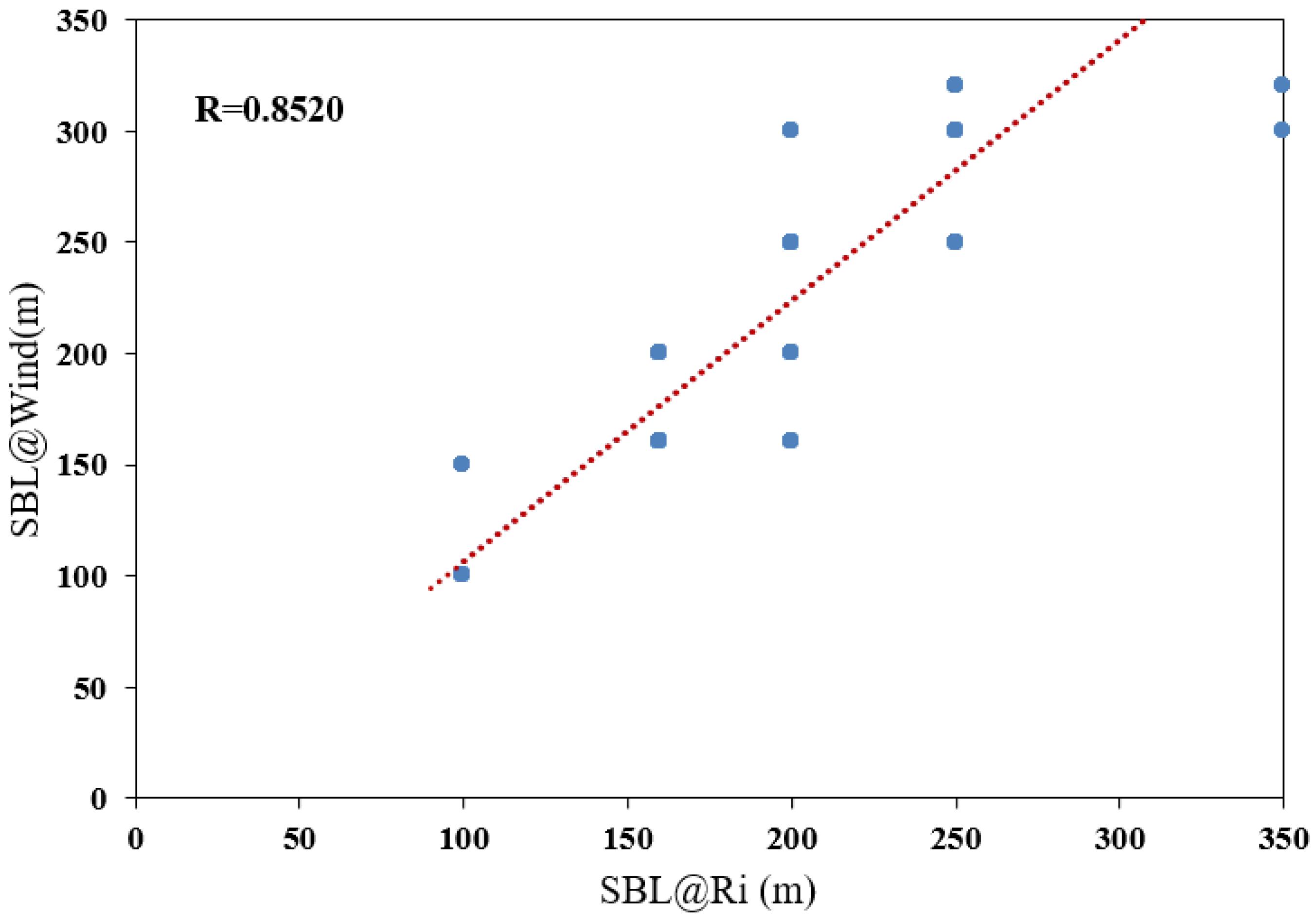
Correlation Coefficient	Average Error (m)	Relative Error (%)
0.8520	27.48	17.17

shows the correlation coefficient and error of both. It can be seen from Figure 3 and Table 2 that the correlation coefficient between them can reach 0.85, the average absolute error is less than 28 m, and the average relative error is less than 18%. This shows that the proposed inversion method has high reliability and accuracy.

3. Results and Discussion

We proposed a method to distinguish different types of wind speed variance profile to solve the problem of misjudgment and missed judgment of the stable boundary layer in Section 2. However, the height of the meteorological gradient observation tower is only 350 m, so the stable boundary layer height above the height of the meteorological gradient observation tower needs to be ascertained via other detection equipment, such as wind lidar. Therefore, it is necessary to extend the model method mentioned above to wind lidar data. From 1 April 2022 to 30 April 2022, a Doppler coherent wind Lidar was placed under the Shenzhen Gradient Observation Tower (113.897°E, 22.649°N), as shown in Figure 4. It is able to obtain wind field information at different altitudes, with a minimum detection altitude of 30 m and a maximum detection altitude of 6 km. The vertical resolution is 15 m and the time resolution is 5 s, as shown in

Table 3. Performance parameters of the wind lidar.

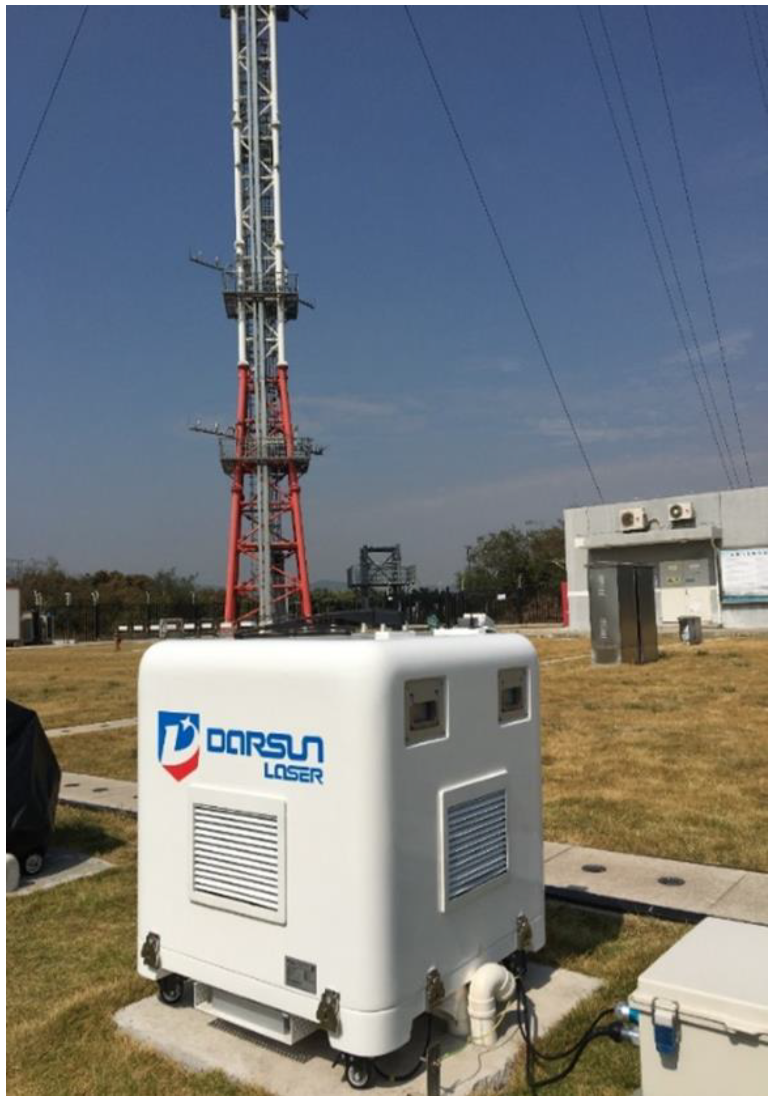
Metrics	Technical Performance Requirements
Minimum detection altitude	≤30 m
Maximum detection altitude	6 km
Distance resolution	15 m
Temporal resolution of wind profile	5 s
Errors of wind speed measurement (standard deviation)	≤0.3 m s−1
Errors of wind direction measurement (root mean squared error)	≤3°
Range of vertical wind speed measurement	0–60 m s−1
Range of wind direction measurement	0°–360°

. The wind lidar can operate continuously over 24 h under clear sky conditions.

Figure 5 shows the wind speed and the corresponding variance of the wind lidar data and the meteorological gradient observation tower data. It can be seen from Figure 5a,b that there is relatively high consistency between their horizontal wind speed measurements. The blind area of wind lidar is 45 m. It can be seen from Figure 5c,d that the variance trends of the two are basically the same, but that of the wind lidar is relatively larger. This is because the wind speed uncertainty of wind lidar is higher, resulting in a higher value of the variance. As can be seen from Figure 2, the method we proposed distinguishes the shape of different variance profiles, which is different from the traditional threshold method, so it is not affected by this factor. Therefore, it is universally applicable to use wind lidar data and the algorithm proposed here to retrieve a stable boundary layer height.

The stable boundary layer algorithm proposed here was applied to wind lidar and the gradient observation tower data, respectively. Figure 6 shows the correlation between the boundary layer below 350 m obtained by the wind lidar and gradient tower observations based on the data from April 2022.

Table 4. Error of the stable boundary layer height obtained by wind lidar.

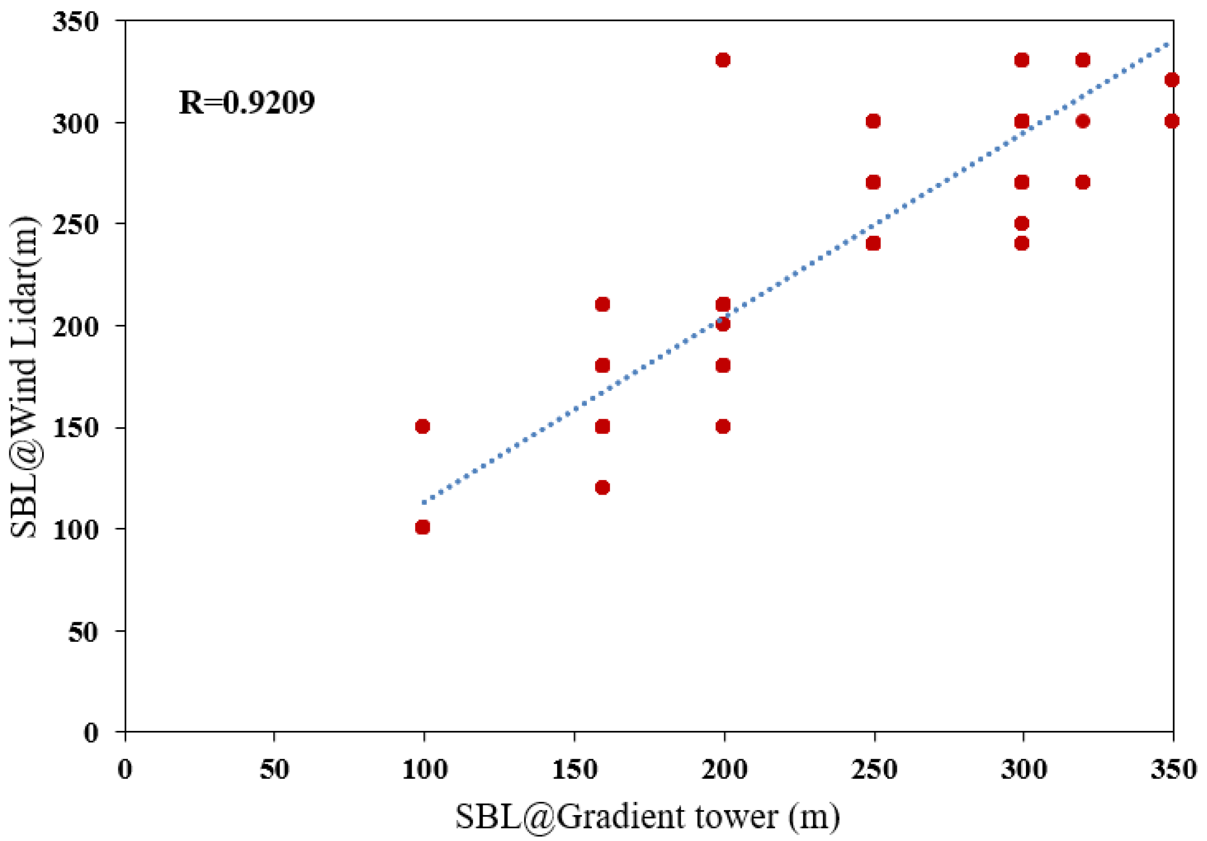
Correlation Coefficient	Average Error (m)	Relative Error (%)
0.9209	17.62	8.21

shows the correlation coefficient and the error. It can be seen from Figure 6 and Table 4 that the correlation coefficient between the two can reach 0.9209, the average absolute error is less than 18 m, and the average relative error is less than 9%. This shows that the proposed inversion method can be extended to the retrieval of the stable boundary layer height with wind lidar data.

The stable boundary layer heights in Shenzhen from April to June 2022 were retrieved using the proposed variance profile shape method, and its distribution characteristics are shown in Figure 7. It can be seen from Figure 7a,b that the distribution of the night stable boundary layer height in April and May is relatively consistent, where the proportions of heights in excess of 350 m are more than 83% and 81%, respectively. It can be seen from Figure 7c that the height distribution of the stable boundary layer in June is different from those in April and May, and it is more concentrated in the interval of 600 to 800 m, where the proportion of heights greater than 350 m is up to about 96%. If only the meteorological gradient observation tower data are used, only the stable boundary layer below 350 m (accounting for about 4%) can be monitored, and the other 96% of the stable boundary layer height cannot be obtained. Using the proposed inversion method of the stable boundary layer height in this paper, the stable boundary layer at any height can be obtained from wind lidar data measured over a long detection distance. This allows us to obtain the height structure characteristics of the stable boundary layer (such as its monthly and seasonal characteristics), which is of great significance.

4. Conclusions

Our research has shown that there are many different vertical variance profiles resulting from low-level jets, and existing research methods have the problems of misjudgment and omission. We put forward a method that utilizes variance profile shapes to retrieve the stable boundary layer height; that is, distinguishing different types of wind speed variance profiles, thus solving the problem of the misjudgment and omission of the stable boundary layer height (about 34%). Due to the low detection range of the gradient observation tower, we extended this method to wind lidar observations, which have a longer detection range. Our experiment shows that the average absolute error of the retrieved stable boundary layer height is less than 18 m and that the average relative error is less than 9%. The results show that the proposed inversion method can be extended to all kinds of wind field detection equipment for inversion of the stable boundary layer height and has very high universality. The proposed retrieval method of the stable boundary layer height has very high application value in environmental meteorological services, climate change response services, numerical prediction services, and other fields.

References

- Yin, J.; Gao, C.Y.; Hong, J.; Gao, Z.; Li, Y.; Li, X.; Fan, S.; Zhu, B. Surface Meteorological Conditions and Boundary Layer Height Variations During an Air Pollution Episode in Nanjing, China. J. Geophys. Res.-Atmos. 2019, 124, 3350–3364. [Google Scholar] [CrossRef]
- Sun, H.J.; Shi, H.R.; Chen, H.Y.; Tang, G.Q.; Sheng, C.; Che, K.; Chen, H.B. Evaluation of a Method for Calculating the Height of the Stable Boundary Layer Based on Wind Profile Lidar and Turbulent Fluxes. Remote Sens. 2021, 13, 3596. [Google Scholar] [CrossRef]
- Peña, A.; Gryning, S.-E.; Hahmann, A.N. Observations of the atmospheric boundary layer height under marine upstream flow conditions at a coastal site. J. Geophys. Res.-Atmos. 2013, 118, 1924–1940. [Google Scholar] [CrossRef]
- Jiang, Q.; Wang, Q. Characteristics and Scaling of the Stable Marine Internal Boundary Layer. J. Geophys. Res.-Atmos. 2021, 126, e2021JD035510. [Google Scholar] [CrossRef]
- Lan, C.; Liu, H.; Katul, G.G.; Li, D.; Finn, D. Turbulence Structures in the Very Stable Boundary Layer Under the Influence of Wind Profile Distortion. J. Geophys. Res.-Atmos. 2022, 127, e2022JD036565. [Google Scholar] [CrossRef]
- Ganeshan, M.; Yang, Y. A Regional Analysis of Factors Affecting the Antarctic Boundary Layer During the Concordiasi Campaign. J. Geophys. Res.-Atmos. 2018, 123, 10830–810841. [Google Scholar] [CrossRef]
- Rey-Sanchez, C.; Wharton, S.; Vilà-Guerau de Arellano, J.; Paw, U.K.T.; Hemes, K.S.; Fuentes, J.D.; Osuna, J.; Szutu, D.; Ribeiro, J.V.; Verfaillie, J.; et al. Evaluation of Atmospheric Boundary Layer Height From Wind Profiling Radar and Slab Models and Its Responses to Seasonality of Land Cover, Subsidence, and Advection. J. Geophys. Res.-Atmos. 2021, 126, e2020JD033775. [Google Scholar] [CrossRef]
- Li, H.; Yang, Y.; Hu, X.-M.; Huang, Z.; Wang, G.; Zhang, B.; Zhang, T. Evaluation of retrieval methods of daytime convective boundary layer height based on lidar data. J. Geophys. Res. Atmos. 2017, 122, 4578–4593. [Google Scholar] [CrossRef]
- Liu, R.; Liu, S.; Huang, H.; Dai, Y.; Zeng, X.; Yuan, H.; Wei, Z.; Lu, X.; Wei, N.; Zhang, S.; et al. The Effect of Surface Heating Heterogeneity on Boundary Layer Height and Its Dependence on Background Wind Speed. J. Geophys. Res.-Atmos. 2022, 127, e2022JD037168. [Google Scholar] [CrossRef]
- Banta, R.M. Stable-boundary-layer regimes from the perspective of the low-level jet. Acta Geophys. 2008, 56, 58–87. [Google Scholar] [CrossRef]
- Banta, R.M.; Mahrt, L.; Vickers, D.; Sun, J.; Balsley, B.B.; Pichugina, Y.L.; Williams, E.J. The Very Stable Boundary Layer on Nights with Weak Low-Level Jets. J. Atmos. Sci. 2007, 64, 3068–3090. [Google Scholar] [CrossRef]
- Banta, R.M.; Pichugina, Y.L.; Brewer, W.A. Turbulent Velocity-Variance Profiles in the Stable Boundary Layer Generated by a Nocturnal Low-Level Jet. J. Atmos. Sci. 2006, 63, 2700–2719. [Google Scholar] [CrossRef]
- Banta, R.M.; Pichugina, Y.L.; Newsom, R.K. Relationship between Low-Level Jet Properties and Turbulence Kinetic Energy in the Nocturnal Stable Boundary Layer. J. Atmos. Sci. 2003, 60, 2549–2555. [Google Scholar] [CrossRef]
- Pichugina, Y.L.; Tucker, S.C.; Banta, R.M.; Brewer, W.A.; Kelley, N.D.; Jonkman, B.J.; Newsom, R.K. Horizontal-Velocity and Variance Measurements in the Stable Boundary Layer Using Doppler Lidar: Sensitivity to Averaging Procedures. J. Atmos. Ocean. Technol. 2008, 25, 1307–1327. [Google Scholar] [CrossRef]
- Moreira, G.D.A.; Marques, M.T.A.; Nakaema, W.; Moreira, A.C.D.C.A.; Landulfo, E. Detecting the planetary boundary layer height from low-level jet with Doppler lidar measurements. In Proceedings of the SPIE Remote Sensing, Toulouse, France, 20 October 2015. [Google Scholar]
- Vickers, D.; Mahrt, A.L. Evaluating Formulations of Stable Boundary Layer Height. J. Appl. Meteorol. 2004, 43, 1736. [Google Scholar] [CrossRef]
- Lemone, M.A.; Tewari, M.; Chen, F.; Dudhia, J. Objectively Determined Fair-Weather NBL Features in ARW-WRF and Their Comparison to CASES-97 Observations. Mon. Weather Rev. 2014, 142, 2709–2732. [Google Scholar] [CrossRef]
- Schween, J.H.; Hirsikko, A.; Lohnert, U.; Crewell, S. Mixing-layer height retrieval with ceilometer and Doppler lidar: From case studies to long-term assessment. Atmos. Meas. Tech. 2014, 7, 3685–3704. [Google Scholar] [CrossRef]
- Shukla, K.K.; Phanikumar, D.V.; Newsom, R.K.; Kumar, K.N.; Ratnam, M.V.; Naja, M.; Singh, N. Estimation of the mixing layer height over a high altitude site in Central Himalayan region by using Doppler lidar. J. Atmos. Sol.-Terr. Phys. 2014, 109, 48–53. [Google Scholar] [CrossRef]
- Stull, R.B. An Introduction to Boundary Layer Meteorology; Springer Science & Business Media: New York, NY, USA, 1988. [Google Scholar]
- Joffre, S.M.; Kangas, M.; Heikinheimo, M.; Kitaigorodskii, S.A. Variability of the stable and unstable atmospheric boundary-layer height and its scales over a boreal forest. Bound.-Layer Meteorol. 2001, 99, 429–450. [Google Scholar] [CrossRef]
- Vogelezang, D.H.P.; Holtslag, A.A.M. Evaluation and model impacts of alternative boundary-layer height formulations. Bound.-Layer Meteorol. 1996, 81, 245–269. [Google Scholar] [CrossRef]
- Seidel, D.J.; Ao, C.O.; Li, K. Estimating climatological planetary boundary layer heights from radiosonde observations: Comparison of methods and uncertainty analysis. J. Geophys. Res.-Atmos. 2010, 115, D16113. [Google Scholar] [CrossRef]
- Seidel, D.J.; Zhang, Y.; Beljaars, A.; Golaz, J.C.; Jacobson, A.R.; Medeiros, B. Climatology of the planetary boundary layer over the continental United States and Europe. J. Geophys. Res. 2012, 117, D17106. [Google Scholar] [CrossRef]
- Nieuwstadt, F.T.M. The Turbulent Structure of the Stable, Nocturnal Boundary Layer. J. Atmos. Sci. 1984, 41, 2202–2216. [Google Scholar] [CrossRef]
- Bonner, W.D. Climatology of the low level jet. Mon. Weather. Rev. 1968, 96, 833–850. [Google Scholar] [CrossRef]