Article

Improving the Accuracy of Flood Susceptibility Prediction by Combining Machine Learning Models and the Expanded Flood Inventory Data

1
Key Laboratory of Regional Ecology and Environmental Change, School of Geography and Information Engineering, China University of Geosciences, Wuhan 430074, China
2
State Key Laboratory of Biogeology and Environmental Geology, China University of Geosciences, Wuhan 430074, China
3
Department of Water Resources, China Institute of Water Resources and Hydropower Research, Beijing 100038, China
*
Author to whom correspondence should be addressed.
Remote Sens. 2023, 15(14), 3601; https://doi.org/10.3390/rs15143601
Submission received: 18 May 2023 / Revised: 10 July 2023 / Accepted: 12 July 2023 / Published: 19 July 2023

Abstract

:
Sufficient historical flood inventory data (FID) are crucial for accurately predicting flood susceptibility using supervised machine learning models. However, historical FID are insufficient in many regions. Remote sensing provides a promising opportunity to expand the FID. However, whether the FID expanded by remote sensing can improve the accuracy of flood susceptibility modeling needs further study. In this study, a framework was proposed for improving the accuracy of flood susceptibility prediction (FSP) by combining machine learning models and the expanded FID using Sentinel-1A radar images. Five widely used machine learning models were employed to verify the accuracy of the proposed method by taking Wuhan City as a case study, including the random forest (RF), gradient boosting decision tree (GBDT), k-nearest neighbor (KNN), support vector machine (SVM), and artificial neural network (ANN) models. Sentinel-1A images from time points before, during, and after flood events were used to expand the FID for training the machine learning models. The results showed that the performance of the machine learning models for predicting flood susceptibility was improved greatly by considering the expanded FID, being improved by approximately 1.14–19.74% based on the area under the receiver operating characteristic curve (AUC). Among the used machine learning models, taking into account all the statistical indicators, the ANN showed the best performance, while the SVM showed the best generalization performance in Wuhan City. According to the results of the ANN model, approximately 19% of the area in Wuhan City, mainly distributed near rivers and lakes, is at a high flood susceptibility level. This study provides an essential reference for flood susceptibility analyses in regions with limited flood sampling data.

1. Introduction

Flood is one of the most common and devastating natural disasters worldwide [1]. According to Rentschler and Salhab (2020) [2], about 23% of the world’s population (about 1.81 billion people) are under the threat of once-in-a-century flood. The global economic losses caused by floods reached USD 82 billion in 2021, accounting for approximately 31% of the global economic losses related to natural disasters [3]. It is certain that floods cannot be avoided. However, in order to reduce the devastating socio-economic impacts, early warning systems have been developed [4] and also operational forecasting and monitoring approaches for flood occurrence applied [5]. The flood disaster losses can be greatly reduced by predicting the probability of flood occurrence in advance using flood susceptibility prediction methods [6].
According to previous studies, there are four types of methods that can be used to predict flood susceptibility, including simple transition methods, knowledge-driven models such as multi-criteria decision-making, hydrological and hydrodynamic models, and data-driven models such as machine learning models [7]. For the simple transition methods and knowledge-driven models (denoted as non-data-driven methods for ease of analysis), the weights of flood conditioning factors are estimated mainly based on expert knowledge [1]. Therefore, many non-data-driven methods are subjective and not easily applied by inexperienced decision-makers. In addition, some non-data-driven methods (such as the frequency ratio method) ignore the internal relationships between flood conditioning factors, which are critical for predicting flood susceptibility in unlabeled pixels accurately. Some hydrological and hydrodynamic models are used for flood susceptibility prediction, although this requires higher data quantity and quality, while the complex calculations require more advanced hardware support. Data-driven machine learning models predict the flood susceptibility in unlabeled pixels by automatically establishing the relationships between the flood conditioning factors and historical flood or non-flood point data [8,9]. They have been widely used in recent years for predicting flood susceptibility, since (1) they are less influenced by subjective experience and can better predict the complex nonlinear relationships between flood events and flood conditioning factors; and (2) they are more flexible because the required data are not complex and are easy to obtain when mapping flood susceptibility. The commonly used machine learning models for FSP include the decision tree (DT), random forest (RF), support vector machine (SVM), artificial neural network (ANN) and deep learning models [8,10,11]. For example, Tehrany et al. (2015) [12] predicted flood susceptibility using SVM models with different kernel functions; Zhao et al. (2020) [13] used convolutional neural networks to predict flood susceptibility; and Li et al. (2023) [14] used the deep learning models coupled with ensemble learning models to model flood susceptibility. These models are widely used in flood susceptibility studies and widely accepted by the scientific community [15]. Despite the advantages of machine learning methods, they depend strongly on sufficient FID as the reference to train and validate the models. However, sufficient FID are difficult to obtain in many global regions, although several global hazard databases, which record flooding events, are publicly accessible, such as the Emergency Disasters Database (EM-DAT), the International Flood Network (IFNET) and the Global Archive of Large Flood Events [16]. The lack of sufficient FID is still one of the biggest challenges limiting the accuracy of machine learning models for FSP, especially in remote or unrecorded regions. Governmental reports, field surveys, and remote sensing data are the most commonly used data sources for obtaining FID [17,18]. Among them, the data from governmental reports and field surveys are more reliable, although the amount of such data (including spatial coverage and integrity) is very limited. Satellite remote sensing provides a significant opportunity to monitor surface water, which can be applied to expand the FID. Synthetic aperture radar (SAR) images with the advantage of penetrating clouds and fogs are considered to be more prominent in monitoring flood-affected areas [19,20]. According to previous studies, Sentinel-1 SAR data are widely used to map floods. For example, Uddin et al. (2019) [21] used multi-temporal Sentinel-1 SAR images to map floods in Bangladesh. Zeng et al. (2020) [22] used Sentinel-1 images to detect the flood disaster in Wuhan in 2016. Yuan et al. (2021) [23] and McCormack et al. (2022) [24] also used Sentinel-1 to extract flood areas.
Some scholars have used the flood areas detected by Sentinel-1 to generate or expand flood inventory data. Shahabi et al. (2020) [18] and Sachdeva et al. (2022) [25] used Sentinel-1 data to extract flood areas to generate FID. Although Sentinel-1 data have advantages in generating flood inventories, satellite monitoring also faces some challenges in extracting flood areas, which affect the accuracy of the expended FID. For example, the small signal backscatter from the flooded surface can be hidden by the double bounce (DB), dielectricity (blocking signal backscatter flow through soil), and vegetation submerged during the flood [26]. These deficiencies may lead to false flood monitoring results, affecting the performance of machine learning models when using the FID generated by remote sensing to predict flood susceptibility in non-monitored regions. Some scholars combined historical FID with the FID generated by remote sensing to generate flood susceptibility maps. Mehravar et al. (2023) [27] combined the historical flood inventory obtained by the agricultural department with the flood inventory generated by Sentinel-1 images to generate flood susceptibility. Shahabi et al. (2020) [18] also used the flood inventory obtained by the water authority and the flood inventory generated by Sentinel-1 images to map the flood susceptibility. However, whether the combination of historical FID and FID generated by remote sensing is an effective way to improve the accuracy of flood susceptibility prediction in areas with sparse historical flood monitoring data needs further study.
This study focuses on proposing a framework to improve the accuracy of FSP by combining widely used machine learning models and the expanded FID based on satellite remote sensing. Wuhan City was selected as a case study for verifying the proposed method. In detail, the FID in Wuhan City were first expanded based on Sentinel-1A images and historical FID. Second, five widely used machine learning models (ANN, RF, GBDT, KNN and SVM) were employed to predict the flood susceptibility index over Wuhan City. Third, the performance of the machine learning models was assessed and compared in two scenarios, i.e., with and without considering the expanded FID. Finally, the impact of the expanded FID on FSP was summarized and relevant uncertainties were discussed.

2. Materials and Methods

2.1. Study Area and Data

2.1.1. Study Area

Wuhan City, with a total area of 8569.15 km2, is located in a transition zone from the hills in Southeastern Hubei Provence to the low mountains and hills at the southern foot of the Dabie Mountains through the eastern edge of the Hanjiang Plain [28]. Therefore, the central area of the city is low and flat, and it is surrounded by north–south hills and ridges. The annual average temperature in Wuhan City is about 15.8–17.5 °C, and the annual average precipitation is about 1150–1450 mm [28,29]. The rainfall is concentrated in the months from June to August every year, accounting for about 40% of the annual rainfall. Figure 1 shows the location of Wuhan City.
There are many rivers, lakes, and ports distributed in Wuhan City. The Yangtze River and the Han River (the largest tributary of the Yangtze River) meet in the center of the city and divide the city into three parts: Hankou, Hanyang, and Wuchang. Many large and small lakes are embedded on both sides of the Yangtze River to form a lake marsh water network. Wuhan has 166 lakes of different sizes, and it is known as the “city of hundreds of lakes”. The annual mean water surface area of the lakes in Wuhan City is about 867 km2 [28]. The abundant precipitation, geographical and topographical factors and the rich river network determine that Wuhan City is extremely prone to flood disaster under extreme rainstorm weather. Since 2010, there have been five serious flood disasters according to the Wuhan Municipal People’s Government. One of them, from 1 July to 6 July 2016, was used as the example to predict the flood susceptibility over Wuhan City.

2.1.2. Data

Three types of data were used in this study, the historical FID, the Sentinel-1A image data used for expanding the FID and the data for calculating the flood conditioning factors for driving the machine learning models. For the historical FID, a total of 77 monitored flood points (FPs), which were provided by the Wuhan Water Authority (http://swj.wuhan.gov.cn/, accessed on 1 July 2023), were used in this study (Figure 1). The historical FID records the exact locations of floods in Wuhan from 2016 to 2022. Most of them were distributed in the central urban area and near rivers. If the centrally distributed FPs in Figure 1 were directly applied to machine learning models for predicting flood susceptibility, it may bring great uncertainties since the data are insufficient and overly concentrated [30].
Sentinel-1A radar images were used to expand the FID based on the historical FID. Sentinel-1A is one of the satellites in the Sentinel-1 satellite series. It carries an imaging C-band SAR instrument and has four imaging modes: Interferometric Wide Swath (IW), Extra-Wide Ewath (EW), Stripmap (SM), and Wave (WV) modes [31,32]. The radar data were used to expand the FID due to their strong ability to penetrate clouds and fogs for reducing the uncertainties caused by cloud and fog disturbances [18]. The cloud, fog, and rain climate phenomena occur frequently during flood periods. Optical images have higher spatial resolution, although they are susceptible to the weather factors [33]. In addition, the temporal resolution of optical images is coarse. The Sentinel-1 Level-1 Ground Range Detected (GRD) products of the IW imaging mode can be downloaded from (https://scihub.copernicus.eu/dhus, accessed on 1 July 2023). Since the flood event used in this study was from 1 July to 6 July 2016, the Sentinel-1A images taken on 30 May, 5 July, and 17 July 2016 were used as the pre-flood disaster image, the middle-flood disaster image, and the post-flood disaster image, respectively. Due to uncontrollable factors, the effective area of the Sentinel-1 images used in this experiment only covers 3417.67 km2 of the study area, accounting for 40.0% of the total area of the study area. The specific distribution of the images is shown in Figure 1.
The data used for calculating the flood conditioning factors include DEM (ASTER GDEM, with vertical and horizontal accuracies of 12.6 m and 72 m, respectively), which were provided by the Geospatial Data Cloud (https://www.gscloud.cn, accessed on 1 July 2023), and land use and soil-type data, which were derived from Tsinghua University (http://data.starcloud.pcl.ac.cn/, accessed on 1 July 2023) and the China Soil Science Data Center (http://vdb3.soil.csdb.cn, accessed on 1 July 2023), respectively. Landsat-8 OLI_TIRS remote sensing images provided by the Geospatial Data Cloud were used to derive the normalized difference vegetation index (NDVI) and normalized difference accumulation index (NDBI).

2.2. Flood Conditioning Factors

The choice of flood regulation factors depends mainly on the characteristics of the study area [34]. Table 1 shows the flood conditioning factors used in this study for deriving the machine learning models to predict the flood susceptibility index over Wuhan City. Based on the geographical and natural environment of Wuhan City and on previous studies, a total of 12 factors were considered, including the elevation, slope, aspect, curvature, NDVI, terrain humidity index (TWI), NDBI, river power index (SPI), land use (LU), soil type (ST), distance to water (DW), and distance type (DT) [8,15,18,35]. Due to the fact that floods are more likely to occur in areas with low and flat terrain [8,9,18], the elevation, slope, aspect, curvature, TWI and SPI have been used in most studies. The coverage of land features and the underlying surfaces with different properties can affect drainage [6]. Thus, the NDVI, LU and ST are used in most studies. Where part of the study area is an urban building area, the NDBI has been added as an conditioning factor in most studies on urban flood susceptibility [3]. The water system has a strong correlation with flood disasters [3,6,8,9]. Therefore, the DW is an important factor chosen to represent water systems in most studies. In addition, this study area is a multi-river and multi-lake area, and in addition to the DW, the DT has been added to distinguish the different types of rivers and lakes. The meanings of these factors and their calculation methods are summarized in Table 1. All these 12 factors were remapped to 30 m spatial resolution.

2.3. Framework and Machine Learning Models for Predicting Flood Susceptibility

Figure 2 shows the proposed flowchart for predicting flood susceptibility using the expanded FID and machine learning models. It includes three key parts: (1) expanding the FID based on Sentinel-1A data (Section 2.3.1); (2) building machine learning models in two scenarios, with and without considering the expanded FID, for predicting flood susceptibility over Wuhan City (Section 2.3.2, Section 2.3.3 and Section 2.3.4); and (3) comparing the performances of different machine learning models for predicting flood susceptibility (Section 2.4).

2.3.1. Methods for Expanding Flood Inventory Data

Sentinel-1A images were employed to expand the FID. The specific steps were as follows. First, Sentinel-1A images from the pre-, middle-, and post-flood periods were prepared for the flood event. These images were pre-processed to extract the water surface area data (before, during and after the flood event), including registration, gamma filtering, geocoding and radiometric calibration. Second, the water surface areas in the pre-, middle-, and post-flood periods were extracted using Otsu’s threshold method (Equation (1)) [22,37]. After many attempts, 48 (the value range is from 0–255) was used as the threshold in this study. The flood area for the flood event (SFlood) is the spatial difference in the water surface area extracted from the Sentinel-1A image during the flood event (SDWA, pre-flood event image) and that extracted from the Sentinel-1A image before the flood event (SBWA, middle-flood event image), i.e., SFlood = SDWA-SBWA. For the misclassification area, the visual interpretation method was used to eliminate the misclassification area caused by the terrain, mainly starting from the landform. The extracted flood area was then compared with the water surface area extracted from the Sentinel-1A image after the flood event (post-flood event image) to reduce the impact of the time interval of shooting the images in the three periods. Finally, FPs were extracted based on the extracted flood areas, which were polygons [9]. These flood polygons were converted into FPs by randomly selecting points at the non-edge locations of the small polygons using ArcGIS 10.6 software. A total of 270 FPs were expanded in this study.
σ 2 = p 1 ( m 1 - m g ) 2 + p 2 ( m 2 - m g ) 2
where σ is the variance between the two categories, p1 and p2 are the proportions of category 1 and category 2 in the image, m1 and m2 are the average values of category 1 and category 2, respectively, and mg is the average value of the whole image. The threshold value when σ2 reaches the maximum value is the best segmentation threshold value.

2.3.2. Data Processing and Scenario Design

The processing of the data included two steps (Figure 2). The first was the selection of non-FPs. According to most previous studies, the non-FPs were randomly selected in the non-flood areas [8,9,38]. The selection method for the non-FPs was to add two constraints on the basis of random selection, one was to avoid the flood area and the other was to select non-FPs within the selected Sentinel-1 image range and the historical flood inventory range. Referring to previous studies, the non-FPs with the same number as the FPs were randomly selected in this study. The second was to determine the test dataset. The test data did participate in the training and verification process during the modeling period. They were only used for the final test of the performances of the models. The numbers of FPs and non-FPs in the test data were equal, accounting for about 20% of all the used points.
Two scenarios were designed for training and validating the machine learning models, i.e., with and without considering the expanded FID (Figure 2). In scenario 1, only the historical FIDs were used to train and validate the models. Specifically, all the historical FIDs except those used for testing the models, including 62 FPs (Figure 2), were used to train and validate the machine learning models, and the same number of non-flood points were selected. Scenario 2 was designed based on scenario 1. We used all the historical FIDs from scenario 1 and all the expanded FIDs except those used for testing the models (216 FPs in total) to train and validate the machine learning models in scenario 2. The same number of non-flood points were also assigned. The test dataset in scenario 2 was the same as that in scenario 1 for a fair comparison.

2.3.3. Machine Learning Models Used in This Study

Five machine learning models were employed in this study, including the ANN, RF, GBDT, KNN, and SVM. Since these models have been described in detail in previous studies, they will be only briefly described. The RF and GBDT models are tree-based integration methods. The RF is based on the decision-making of multivariate trees, that is, its result is decided by a majority vote [39]. Majority voting enables the RF to handle the overfitting problem and interpret the complex relationship between the conditioning factors. The GBDT is a decision tree algorithm based on a boosting algorithm [40]. Different from the RF bagging algorithm, the boosting algorithm is the decision result of all the trees. The RF and GBDT are widely used in studies concerning flood susceptibility prediction due to their interpretability and high accuracy.
The KNN algorithm, originally proposed by Cover and Hart in 1968, is one of the most typical machine learning algorithms [18]. According to the algorithm, if most of the K-adjacent samples for a certain sample belong to a certain category, the sample is considered to belong to that category [41]. The advantage of the KNN lies in its simplicity, effectiveness, and ability to handle complex nonlinear relationships.
The SVM is a supervised machine learning model, which maps the original data to a high-dimensional space and then constructs a hyperplane through a kernel function to convert nonlinear relations into linear relations, thus simplifying the classification [12,42]. The key to building the SVM is the choice of kernel function, which affects the accuracy of the model. According to previous studies, the best performing RBF was selected as the kernel function of this model [12,42,43]. The SVM has strong generalization ability and good performance in processing high-dimensional data.
The ANN is an information processing system based on the structure and function of brain neural networks. It simulates the activity of neurons based on mathematical models. The neural network is widely used in flood susceptibility modeling. A deep neural network (DNN) is an ANN with multiple hidden layers, which is effective in dealing with the complex relationship between flood and flood conditioning factors [44]. The ANN has excellent abilities in terms of learning complex linear relationships and applying various types of data.
In this study, a total of ten machine learning models were constructed (each scenario included five models) (Figure 2).

2.3.4. Steps for Predicting Flood Susceptibility Using Machine Learning Models and the Expanded FID

The steps for predicting flood susceptibility using the machine learning models can be summarized as follows. First, the flood and non-flood points in Wuhan City were labeled 1 and 0, respectively. They represented a 100% probability of flood occurrence and non-occurrence, respectively. The flood conditioning factors representing the classification (soil type, land use and distance type) were quantified, and natural numbers were used to replace their classification. Before being incorporated into the model, the values of the 12 flood conditioning factors were normalized to adapt to models that require feature normalization, such as the KNN, Ann and SVM. The data concerning the selected 12 flood conditioning factors (Table 1) were prepared for driving the machine learning models to predict the flood susceptibility index (varying between 0 and 1) in the unlabeled regions over the study area. Second, the different machine learning models were built and trained based on the designed scenarios in Section 2.3.2 and the data preparation in the first step to predict the flood susceptibility index over Wuhan City. For the RF, GBDT, KNN, and SVM models, they were built based on Python’s Scikit-Learn package. For the ANN model, it was built based on PyTorch for building a neural network framework. Then, the models were trained using cross-validation and spatial cross-validation methods to evaluate the models more accurately. We used 5-fold cross-validation and 5-fold spatial cross-validation, where k-means clustering was used for the data partitioning in the spatial cross-validation [45]. Finally, the flood susceptibility index in the unlabeled pixels over Wuhan City was predicted based on the trained machine learning models. The performances of the different machine learning models were compared in the designed two scenarios based on the statistical metrics in Section 2.4. Based on the results of the performance comparison of the machine learning models, flood susceptibility maps of Wuhan City were mapped.

2.4. Statistical Metrics

Six statistical metrics were selected to measure the performances of the different machine learning models for FSP, including the receiver operating characteristic curve (ROC), the area under the ROC curve (AUC), the Kappa coefficient, precision, recall and F1-score [8,14,46]. The ROC and AUC are the most commonly used metrics to measure model performance for FSP. The ROC takes the true and false positive rates as the vertical and horizontal axes, respectively. The closer the curve is to the upper left corner, the higher the model performance is. The area under the ROC curve (AUC) varies between 0.5 and 1 [14]. The closer to 1 the AUC value is, the better the model performance is. The Kappa coefficient varies between −1 and 1. The closer to 1 the value is, the more consistent the predicted and observed values are [46]. Precision and recall are metrics used in machine learning to measure the accuracy of a classification model. Precision focuses on the correctness of the positive predictions, while recall focuses on the model’s ability to identify all the positive instances correctly [8]. The F1-score is a metric that combines precision and recall to provide a balanced evaluation of a classification model. It is the harmonic mean of the precision and recall, and it takes both false positives and false negatives into account. The ROC curve and AUC value are the most commonly used indicators for binary classification tasks in machine learning. A higher recall rate means that there are fewer omissions in the identification of flood-prone areas. Therefore, in Section 3.4, the test performance comparison of the models mainly compares the AUC value and recall rate of the models.
Recall = TPR = TP TP + FN
FPR = FP FP + TN
Precision = TP TP + FP
K = O-E 1-E
E = TP + FP N × TP + FN N + TN + FP N × TN + FN N
F = 2 × Recall × Precision Recall + Precision
where TP (true positive) and TN (true negative) represent the number of points correctly classified as flood and non-flood, respectively; FP (false positive) and FN (false negative) are opposite to TP and FP, respectively; K and N refer to the kappa coefficient and the number of all the sample data, respectively; and F refers to the F1-score.

2.5. Analysis of Appearance Rationality of Susceptibility Mapping

The flood susceptibility maps generated by the different models may have different spatial patterns. Therefore, we used the method of generating a variability map combined with the conditioning factors to analyze the flood-prone mutation region subjectively, so as to make the results more convincing [47]. The variability value was obtained by calculating the rate of change of a pixel and its surrounding 3 × 3 pixels [47]. The change rate of the three grids was calculated, and the generation method was to use the local statistical tool in ArcGIS software to calculate the variability.

3. Results

3.1. Expansion of Flood and Non-Flood Points

As a typical representative of a multi-river and -lake city, Wuhan City should fully consider the changes in the water surface area of lakes and rivers over time when extracting flood areas. In this study, we considered the changes in the water surface area of lakes and rivers before and after the flood period to eliminate the impact of the changes on the area of rivers and lakes.
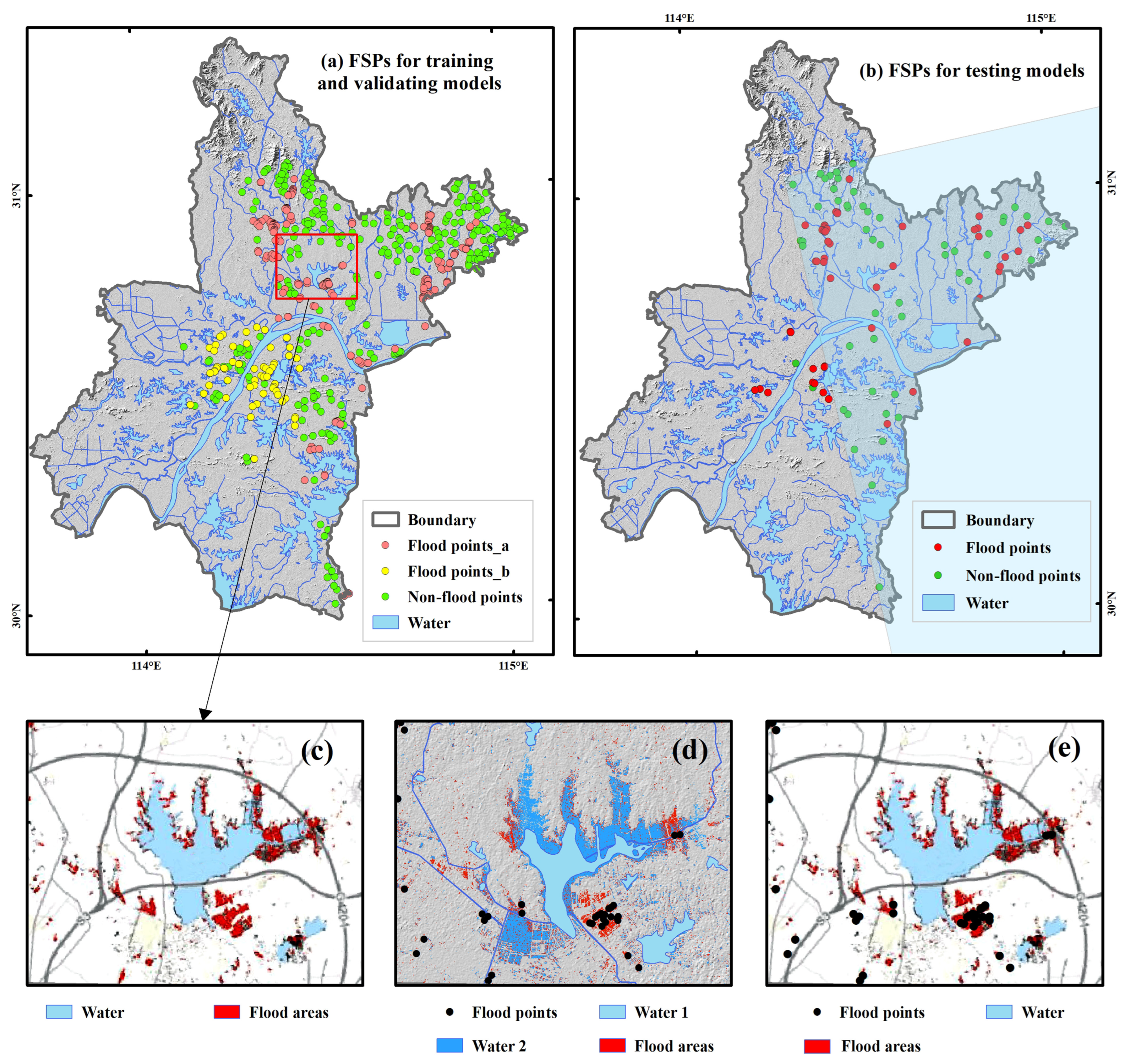
Figure 3a,b show the historical and expanded flood and non-flood point data used for training, validating and testing the machine learning models. It is clear that the historical FPs are mainly distributed in the central areas of Wuhan City. In addition, most of them are distributed near rivers and lakes. It is obvious that the historical flood point data are not sufficient for flood susceptibility prediction using machine learning models in Wuhan City. The expanded flood point data have better spatial representation.
The accuracy of the expanded flood point data in this study was verified by comparing them with the flood point data expanded by previous studies. Figure 3c shows the extraction of the flood area by Zeng et al. (2022) [22] near Wu Lake. Zeng et al. used the Otsu method to extract the flood area of Sentinel-1 images of the same flood event as this study. The producer’s accuracy and the user’s accuracy in the flood areas extracted by Zeng et al. (2022) reached 72.8% and 74.4%, respectively. The area near Wu Lake was selected as an example for the verification (Figure 3c–e). On the one hand, the spatial distribution of the flood areas extracted by Zeng et al. (2020) [22] (Figure 3c) and that extracted in this study (Figure 3d) is highly overlapped. On the other hand, we compared the spatial locations of the FPs extracted in this study (Figure 3d) and those extracted based on the flood areas identified by Zeng et al. (2020) [22] (Figure 3e). The results showed that 95% of the FPs extracted in this study are spatially overlapped with those extracted based on the identified flood area by Zeng et al. (2020) [22]. This shows that the FPs extracted in this study are reasonable.

3.2. Multicollinearity of Flood Conditioning Factors

When selecting conditioning factors, a multicollinearity check shall be conducted [48]. This section focuses on assessing the multicollinearity of the selected flood conditioning factors using the variance inflation factor (VIF) [49]. The VIF is the ratio of variance between a model constructed with multiple other parameters and a model constructed with only one item. It quantifies the severity of the multicollinearity in an ordinary least squares regression analysis. When there is no multicollinearity, the value of the VIF is close to 1. According to previous studies, when the VIF value is greater than 10, it indicates a serious multicollinearity problem [15]. High correlation between the flood conditioning factors affects the performance of the machine learning models. Figure 4 shows the spatial distribution of the selected 12 flood conditioning factors in Wuhan City. Table 2 shows the specific classification names of three flood conditioning factors represented by classification. Table 3 shows the VIFs of these factors.
It can be seen from Table 3 that the VIFs for most of the flood conditioning factors are less than 10, except for the distance type factor with a VIF of 11.83, which is slightly greater than 10. As Wuhan is a region with many lakes and rivers, in addition to the distance from the rivers and lakes, the diversity of the rivers and lakes means that different types of rivers and lakes will have different effects on the occurrence of floods. We used the Euclidean distance to classify the nearest water type (river and lake) of the pixel to be predicted, because different types of waters have different effects on the risk of flood. Because there is still a lack of relevant research on flood susceptibility mapping in areas with many rivers and lakes, in addition to this conditioning factor, no more suitable conditioning factor has been found. Thus, to sum up, even if the VIF of the distance-type factor is greater than 10, it is still applied to this study.

3.3. Training and Validation of Machine Learning Models

This study employed five machine learning models (ANN, RF, GBDT, KNN, and SVM). Based on two scenarios (with and without considering expanding FID; see Section 2.3.2 for details), the five-fold cross-validation and the five-fold spatial cross-validation methods were adopted for training and validation purposes. Table 4 shows the hyperparameters after parameter adjustment. The adjusted AUC values were used to measure the performances of the machine learning models (Table 5). The ANN model used in this study adopted a fully connected layer structure with 1 input layer including 12 ganglion points and 4 hidden layers including 24, 15, 10, and 5 ganglion points, respectively.
According to Table 5, when the cross-validation method is used, the ANN model shows the best performance in the scenario without considering the expanded FID (scenario 1, with an AUC value of 0.97), followed by the GBDT, RF and SVM models (with AUC values of 0.90, 0.89 and 0.87, respectively), whereas the KNN model shows the worst performance according to the AUC (with a value of 0.83). In the scenario with considering the expanded FID (scenario 2), the ANN model also shows the best performance in Wuhan City, with an AUC value of 0.94, followed by the SVM, GBDT and RF models (with AUC values of 0.92, 0.92 and 0.90, respectively). The KNN model (with an AUC value of 0.89) shows the worst performance in scenario 2, as that in scenario 1. When the spatial cross-validation method is used, the GBDT model shows the best performance in the scenario without considering the expanded FID (scenario 1, with an AUC value of 0.98), followed by the RF and ANN models (with AUC values of 0.97 and 0.92, respectively), whereas the KNN and SVM models show the worst performance according to the AUC (with a value of 0.82). In the scenario with considering the expanded FID (scenario 2), the RF and GBDT models show the best performance in Wuhan City, with an AUC value of 0.95, followed by the ANN and SVM models (with AUC values of 0.89 and 0.86, respectively). The KNN model (with an AUC value of 0.81) shows the worst performance in scenario 2, as that in scenario 1. Therefore, the GBDT model performs the best for flood susceptibility prediction in Wuhan City. Note that all five models used in this study show satisfactory performance in both scenarios, with and without considering the expanded FID, in Wuhan City (the AUC values of all these models are greater than 0.8 in the validation period), although these models show different performances.

3.4. Performance Comparison of Machine Learning Models

This section focuses on (1) assessing whether the performance of FSP is improved by considering the expanded FID based on the selected five machine learning models, and (2) comparing the performance differences of the selected five machine learning models for predicting flood susceptibility. In order to provide a fair comparison, the data concerning the FPs used for testing the models’ performance did not include the FPs data used for training and validating the models (Figure 2). In addition, all the models (with and without considering the expanded FID) used the same test dataset to remove the impact of inconsistent test datasets. Figure 5 and Table 6 show the statistical metrics used for assessing the performances of the machine learning models, including the ROC curves, AUC, Kappa coefficient, precision, recall, F1-score and the improvement in the AUC.
As for AUC value, in the test phase, only the SVM (with AUC = 0.88) and ANN (with AUC = 0.83) show good AUC values among the data modeling models using scenario 1, while the AUC values of other models are very low, which could not meet the requirements. In the model of the scenario 2 data modeling, all the models generally show good performance. Specifically, the RF (with AUC = 0.93) has the best performance, followed by the GBDT (with AUC = 0.91), ANN (with AUC = 0.91), and SVM (with AUC = 0.89), while the KNN (with AUC = 0.86) has the lowest AUC value. In terms of the recall rate, in the simulated data of scenario 1, the ANN (with recall = 0.79) shows the highest recall rate, followed by the SVM (with recall = 0.76). In the simulated data of scenario 2, the ANN (with recall = 0.91) still has the highest recall rate, followed by the RF (with recall = 0.86), GBDT (with recall = 0.85), and KNN (with recall = 0.83), while the SVM (with recall = 0.76) performs the worst.
Comparing the simulation models of scenario 1 and scenario 2, we find that the AUC value of the GBDT has the largest difference. The GBDT model in scenario 2 shows a 19.74% increase in the AUC compared to the model in scenario 1. The RF (with an improvement in the AUC = 16.25%), KNN (with an improvement in the AUC = 11.69%), and ANN (with an improvement in the AUC = 9.64%) take second place, while the SVM (with an improvement in the AUC = 1.14%) has the smallest AUC difference. This indicates that the SVM model has stronger generalization performance compared to other models, while the GBDT and RF exhibit significant overfitting phenomena. This means that when modeling with insufficient FID, the GBDT and RF models are not suitable due to overfitting issues. On the contrary, the SVM model is more suitable for modeling in situations where the FID are scarce. Based on the above results, the ANN model exhibits good comprehensive performance, with no obvious overfitting phenomenon when modeling in both scarce and sufficient data, and its recall rate is the highest in both scenario 1 and scenario 2. The SVM model is more suitable for modeling in FID-scarce areas, which helps to reduce the overfitting effects caused by data scarcity. However, due to its low recall rate, the SVM is not suitable for modeling when the FID are sufficient.

3.5. Flood Susceptibility Map and Appearance Rationality Analysis in Wuhan City

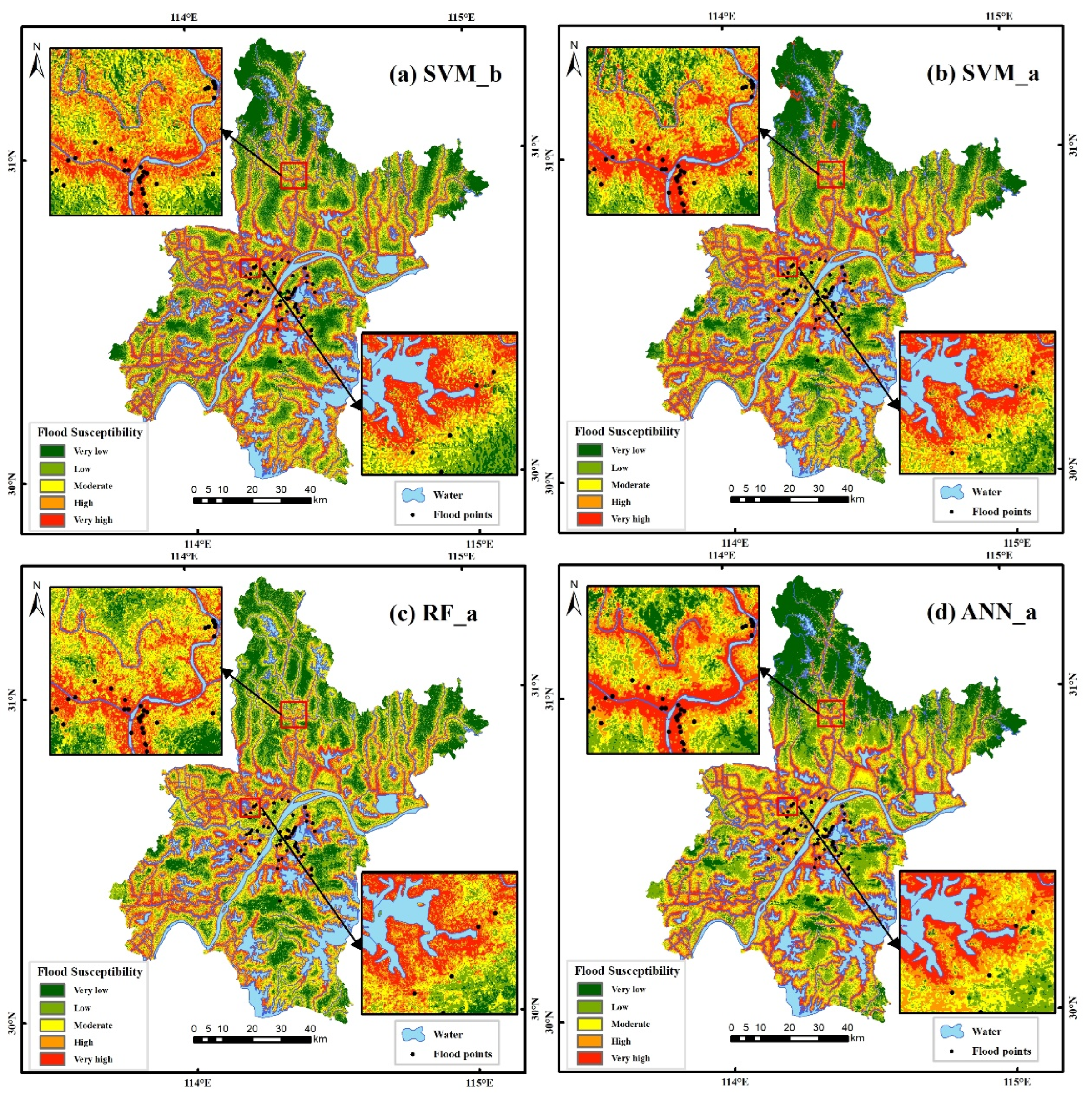
Figure 6 shows the flood susceptibility maps of Wuhan City based on the SVM, RF and ANN models. Since the SVM model shows a better performance based on results in Section 3.4, the flood susceptibility map predicted by the SVM model is used to analyze the flood susceptibility in Wuhan City. The susceptibility maps predicted by the RF and ANN models are also considered for inter-comparison purposes. The flood susceptibility index varying between 0 and 1 in Figure 6 is used to represent the probability of flood occurrence. Five levels of flood susceptibility are divided based on the flood susceptibility index using the quantile method, including very low, low, moderate, high, and very high. The area and its proportion for each level are plotted in Figure 7.
According to Figure 6 and Figure 7, about 70% of the historical FPs are located within areas with high or very high flood susceptibility levels, while less than 20% of the historical FPs are located within areas with very low or low flood susceptibility levels. According to Figure 7, nearly 36% of areas in Wuhan City are at high and very high flood susceptibility levels, of which approximately 19% are at a very high susceptibility level. This means that 36% of areas in Wuhan City will be at risk of flooding when extreme rainfall occurs and 19% of areas are in the high flood risk state. These places are mainly distributed in regions near low-lying rivers and lakes. The percentages for the very low, low and moderate flood susceptibility levels are 17%, 24% and 23%, respectively.
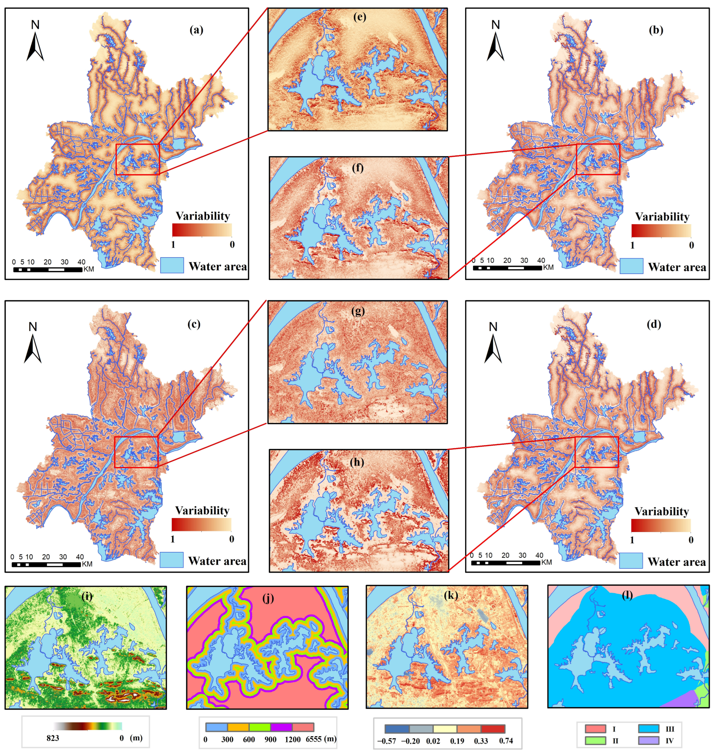
Figure 8 shows the variability map generated by the flood susceptibility map in Figure 7 as well as some important conditioning factors. It is possible to analyze the rationality of the generated flood susceptibility map by combining four important conditioning factors (elevation, distance from water body, distance type, and NDVI). After the comparison, we find that areas with sudden changes in susceptibility are located in areas with higher elevations and sudden changes, as well as in areas close to rivers and lakes. This is consistent with the phenomenon that floods usually occur in areas close to rivers and lakes and in low-lying areas, while they are not easy to occur in areas with larger slopes. Interestingly, the distance between the sensitive mutation areas and rivers and lakes also varies. The distance between the sensitive mutation area and the lake is obviously greater than the distance from the Yangtze River. This indicates that the area around the Yangtze River is less affected by floods than lakes. It shows that the lake area needs to strengthen its flood management.

4. Discussion

In this study, we used Sentinel-1A radar data to expand the FID in Wuhan City. The results showed that the expanded data can improve the performances of the machine learning models well. That is, the performances of all five models has been improved by considering the expanded FID compared to the performances when not considering the data expansion. The performance improvement is caused mainly by the increased sample size (e.g., the number of FPs). According to Zhao et al. (2021) [50], the model performance for predicting flood susceptibility will be improved as the number of samples increases. However, if the expanded FID are not corrected (such as the non-flood points are incorrectly used as flood points), the model performance will be decreased as the number of FP samples increases. Our results showed the reliability of the expanded FID based on Sentinel-1A data for improving the performance of FSP using machine learning models. Another reason for the increased model performance is that the expanded and historical FPs are evenly distributed over the study area, meaning that the distance between the predicting cells and their corresponding training domains is greatly decreased. According to McCartney et al. (2020) [51], the model performance will be improved rapidly as the distance of the predicting cells from their training domains decreases. Note that the expanded FPs in this study were not distributed in all the regions of the study area, because Sentinel-1A covers only half of the study area during the disaster event (the east half of the study area). This brings uncertainties to the results of this study concerning flood susceptibility prediction.
Despite the advantages, the data expansion based on Sentinel-1 data faces some limitations. First, Sentinel-1 data are difficult to use to extract the water surface area in urban areas due to the double bounce mechanism of radar remote sensing in urban areas [52,53], although they can be well used to extract the water bodies in bare land and sparsely vegetated areas due to the obvious backscattering characteristics of water bodies [52]. Some previous studies extracted flood area data in urban areas based on datasets from the TerraSAR-X and ALOS-2/PALSAR-2 synthetic aperture radar sensors [53]. The spatial resolution of the datasets derived from these sensors is no more than 3 m. However, the spatial resolution of Sentinel-1 data is 5 × 20 m, making it difficult to accurately extract water bodies in urban areas. Second, the vegetation canopy cannot be penetrated by Sentinel-1 sensors, which leads to abnormalities in the water surface extraction in densely vegetated areas [22]. In addition, the rapid flow of water during the flood period will also lead to water detection errors [53]. Third, the temporal resolution of Sentinel-1A images is not enough for monitoring flood processes dynamically. For the flood event in this study (during 1 July to 6 July 2016), only one Sentinel-1A image is available (the imaging date is 5 July 2016) during the event, which affects the accuracy of this study. If more images during flood events can be considered, the accuracy of the machine learning models may be further improved. In the future, multi-source remote sensing images can be combined to more accurately extract the flood areas.
The Otsu threshold method has certain limitations when extracting water bodies from Sentinel-1 images. The Otsu threshold method can quickly and conveniently calculate the threshold for image segmentation [54]. For threshold images with a unimodal histogram distribution, the Otsu threshold method has good results, although it is difficult for the Otsu method to achieve a good effect for threshold images with a bimodal or multimodal histogram distribution [55]. In addition, when the water area is less than 10%, there will be significant deviation in the segmentation results [56]. We used a VV polarized Sentinel-1 image, which is a threshold image with a bimodal histogram distribution, which can lead to certain deviations when extracting water bodies. For example, some areas with undulating terrain may be mistakenly classified as water bodies due to the terrain and beam incidence angle. Therefore, we used visual interpretation to eliminate some misclassification areas, although we were unable to take into account all the misclassification areas. Therefore, our goal is to select flood points as accurately as possible to compensate for the shortcomings of the water area extraction. In addition, the area of lakes and rivers in the study area of this experiment is about 26.1%, which excludes the deviation caused by the water body area being less than 10%.
The selection of the test set data points in this experiment has certain limitations. In order to ensure that the test set can contain richer information, we chose the test set data based on the spatial distribution and density of the points. This method ensures that the points in the test set are more dispersed in space, providing richer information for the model performance evaluation. Therefore, our test results will better reflect the generalization and robustness of the model. However, this method does overlook the imbalance in the number of points between the historical flood inventory and the remote sensing flood inventory in the test set. This will cause the test results to be more biased toward the expanded FID data, leading to uncertainty in the results. In future research work, the selection of the testing machines needs to balance the spatial distribution of the historical FID and the expanded FID with the proportion of the sample size, which will make the results more convincing.
When comparing the different machine learning models, they showed different generalizations and accuracies, which are critical for accurate FSP in regions with insufficient historical FID. Based on most previous studies, semi-supervised models have stronger generalization than supervised models when predicting flood susceptibility [40,50,57,58], since supervised models rely more on the quality of the sampling data (the number and spatial distribution of the FPs). Transfer learning is also an important approach for reducing the model generalization in areas with sparse FID. The transfer learning models were trained in areas with sufficient FID and similar environmental conditions as the study area first, and then they were trained again in the study area with insufficient FID to improve the generalization and ability of the models [50]. In addition, the imbalanced size between the flood and non-flood points is another factor affecting the model performance and generalization [40]. Ekmekcioğlu et al. (2022) [8] found that when the number of flood points is equal to that of the non-flood points, the model shows a better performance. However, when the number of flood and non-flood points is seriously imbalanced, the model performance will be reduced significantly. In future research, semi-supervised learning will be an important method to improve the accuracy of flood susceptibility modeling in FID-scarce areas.
Our flood susceptibility map shows that most flood-prone areas are located in areas with low elevations, flat terrain, and close to water bodies. This is consistent with most studies. In addition, most of the susceptible areas in this study are more densely distributed around water bodies, which is different from some studies [8]. This is because our study area is an area with many lakes and rivers. This is consistent with the results concerning the same study area with a large number of lakes and rivers [34,59].

5. Conclusions

The purpose of this study was to propose a framework for improving the performance of FSP by combining machine learning models and the expanded FID based on satellite remote sensing. Wuhan City was selected as a case study and five widely used machine learning models were employed to verify the proposed method and compare their performance differences in two scenarios, with and without considering the expanded FID, including the RF, GBDT, KNN, SVM, and ANN. The main conclusions obtained in this study can be summarized as follows.
The expanded FID based on Sentinel-1A data greatly improved the performance of the machine learning models for flood susceptibility prediction in Wuhan City, improving by approximately 1.14~19.74% the statistical metrics of AUC. The ANN model showed the best performance in all scenarios. The SVM model showed a better reducing the overfitting caused by insufficient FPs. According to the flood susceptibility map of Wuhan City, about 36% of areas in Wuhan City are at the risk of flooding. Among them, 19% are at the high susceptibility risk level. These high-risk regions are mainly distributed in regions near low-lying rivers and lakes. Although increasing the number of FPs can improve the performance of machine learning models for FSP, it is affected by the quality of the expanded FID since the water surface extraction based on Sentinel-1A data is limited by the vegetation canopy, urban land, and the temporal and spatial resolution of the Sentinel-1A data. When using SAR images to generate FID, it is necessary to eliminate the impacts of seasonal changes in water bodies and to select a more accurate water extraction method for images with a bimodal histogram distribution. The combination of the expanded FID and transfer learning models may be an effective way to further improve the accuracy of flood susceptibility prediction.

Author Contributions

Conceptualization, H.Y. and Z.L.; methodology, H.Y. and Z.L.; validation, H.Y. and Z.L.; formal analysis, H.Y. and Z.L.; investigation, H.Y.; resources, Z.L., L.W. and X.D.; data curation, L.W. and X.D.; writing—original draft preparation, H.Y.; writing—review and editing, Z.L. and H.Y.; visualization, H.Y.; supervision, Z.L., L.W., X.D. and S.W.; project administration, L.W. All authors have read and agreed to the published version of the manuscript.

Funding

This research was funded by National Natural Science Foundation of China (No.42201038).

Data Availability Statement

The data for this article are freely available at https://www.gscloud.cn (accessed on 1 July 2023), http://swj.wuhan.gov.cn/ (accessed on 1 July 2023), https://scihub.copernicus.eu/dhus (accessed on 1 July 2023), http://data.starcloud.pcl.ac.cn/ (accessed on 1 July 2023) and http://vdb3.soil.csdb.cn (accessed on 1 July 2023).

Acknowledgments

We are very grateful to the journal editors and anonymous reviewers for their insightful comments and great efforts on this paper.

Conflicts of Interest

The authors declare no conflict of interest.

References

  1. Chen, W.; Hong, H.; Li, S.; Shahabi, H.; Wang, Y.; Wang, X.; Ahmad, B.B. Flood susceptibility modelling using novel hybrid approach of reduced-error pruning trees with bagging and random subspace ensembles. J. Hydrol. 2019, 575, 864–873. [Google Scholar] [CrossRef]
  2. Rentschler, J.; Salhab, M. People in Harm’s Way: Flood Exposure and Poverty in 189 Countries; The World Bank: Washington, DC, USA, 2020. [Google Scholar]
  3. Fu, S.; Lyu, H.; Wang, Z.; Hao, X.; Zhang, C. Extracting historical flood locations from news media data by the named entity recognition (NER) model to assess urban flood susceptibility. J. Hydrol. 2022, 612, 128312. [Google Scholar] [CrossRef]
  4. Esposito, M.; Palma, L.; Belli, A.; Sabbatini, L.; Pierleoni, P. Recent advances in internet of things solutions for early warning systems: A review. Sensors 2022, 22, 2124. [Google Scholar] [CrossRef] [PubMed]
  5. Giannaros, C.; Dafis, S.; Stefanidis, S.; Giannaros, T.M.; Koletsis, I.; Oikonomou, C. Hydrometeorological analysis of a flash flood event in an ungauged Mediterranean watershed under an operational forecasting and monitoring context. Meteorol. Appl. 2022, 29, e2079. [Google Scholar] [CrossRef]
  6. Wang, Y.; Hong, H.; Chen, W.; Li, S.; Panahi, M.; Khosravi, K.; Shirzadi, A.; Shahabi, H.; Panahi, S.; Costache, R. Flood susceptibility mapping in Dingnan County (China) using adaptive neuro-fuzzy inference system with biogeography based optimization and imperialistic competitive algorithm. J. Environ. Manag. 2019, 247, 712–729. [Google Scholar] [CrossRef]
  7. Al-Abadi, A.M.; Pradhan, B. In flood susceptibility assessment, is it scientifically correct to represent flood events as a point vector format and create flood inventory map? J. Hydrol. 2020, 590, 125475. [Google Scholar] [CrossRef]
  8. Ekmekcioğlu, Ö.; Koc, K.; Özger, M.; Işık, Z. Exploring the additional value of class imbalance distributions on interpretable flash flood susceptibility prediction in the Black Warrior River basin, Alabama, United States. J. Hydrol. 2022, 610, 127877. [Google Scholar] [CrossRef]
  9. Fang, Z.; Wang, Y.; Peng, L.; Hong, H. Predicting flood susceptibility using LSTM neural networks. J. Hydrol. 2021, 594, 125734. [Google Scholar] [CrossRef]
  10. Wang, Y.; Fang, Z.; Hong, H.; Peng, L. Flood susceptibility mapping using convolutional neural network frameworks. J. Hydrol. 2020, 582, 124482. [Google Scholar] [CrossRef]
  11. Merz, B.; Thieken, A.H.; Gocht, M. Flood risk mapping at the local scale: Concepts and challenges. Adv. Nat. Technol. Hazards Res. 2007, 25, 231–251. [Google Scholar] [CrossRef]
  12. Tehrany, M.S.; Pradhan, B.; Mansor, S.; Ahmad, N. Flood susceptibility assessment using GIS-based support vector machine model with different kernel types. Catena 2015, 125, 91–101. [Google Scholar] [CrossRef]
  13. Zhao, G.; Pang, B.; Xu, Z.; Peng, D.; Zuo, D. Urban flood susceptibility assessment based on convolutional neural networks. J. Hydrol. 2020, 590, 125235. [Google Scholar] [CrossRef]
  14. Li, Y.; Hong, H. Modelling flood susceptibility based on deep learning coupling with ensemble learning models. J. Environ. Manag. 2023, 325, 116450. [Google Scholar] [CrossRef]
  15. Saha, T.K.; Pal, S.; Talukdar, S.; Debanshi, S.; Khatun, R.; Singha, P.; Mandal, I. How far spatial resolution affects the ensemble machine learning based flood susceptibility prediction in data sparse region. J. Environ. Manag. 2021, 297, 113344. [Google Scholar] [CrossRef] [PubMed]
  16. Adhikari, P.; Hong, Y.; Douglas, K.R.; Kirschbaum, D.B.; Gourley, J.; Adler, R.; Brakenridge, G.R. A digitized global flood inventory (1998–2008): Compilation and preliminary results. Nat. Hazards 2010, 55, 405–422. [Google Scholar] [CrossRef]
  17. Hong, H.; Panahi, M.; Shirzadi, A.; Ma, T.; Liu, J.; Zhu, A.X.; Chen, W.; Kougias, I.; Kazakis, N. Flood susceptibility assessment in Hengfeng area coupling adaptive neuro-fuzzy inference system with genetic algorithm and differential evolution. Sci. Total Environ. 2018, 621, 1124–1141. [Google Scholar] [CrossRef]
  18. Shahabi, H.; Shirzadi, A.; Ghaderi, K.; Omidvar, E.; Al-Ansari, N.; Clague, J.J.; Geertsema, M.; Khosravi, K.; Amini, A.; Bahrami, S.; et al. Flood detection and susceptibility mapping using Sentinel-1 remote sensing data and a machine learning approach: Hybrid intelligence of bagging ensemble based on K-Nearest Neighbor classifier. Remote Sens. 2020, 12, 266. [Google Scholar] [CrossRef] [Green Version]
  19. Zhang, X.; Chan, N.W.; Pan, B.; Ge, X.; Yang, H. Mapping flood by the object-based method using backscattering coefficient and interference coherence of Sentinel-1 time series. Sci. Total Environ. 2021, 794, 148388. [Google Scholar] [CrossRef]
  20. Huth, J.; Gessner, U.; Klein, I.; Yesou, H.; Lai, X.; Oppelt, N.; Kuenzer, C. Analyzing water dynamics based on sentinel-1 time series-a study for dongting lakewetlands in China. Remote Sens. 2020, 12, 1761. [Google Scholar] [CrossRef]
  21. Uddin, K.; Matin, M.A.; Meyer, F.J. Operational flood mapping using multi-temporal Sentinel-1 SAR images: A case study from Bangladesh. Remote Sens. 2019, 11, 1581. [Google Scholar] [CrossRef] [Green Version]
  22. Zeng, Z.; Gan, Y.; Kettner, A.J.; Yang, Q.; Zeng, C.; Brakenridge, G.R.; Hong, Y. Towards high resolution flood monitoring: An integrated methodology using passive microwave brightness temperatures and Sentinel synthetic aperture radar imagery. J. Hydrol. 2020, 582, 124377. [Google Scholar] [CrossRef]
  23. Yuan, X.; Zhang, X.c.; Wang, X.g.; Zhang, Y. Flood disaster monitoring based on Sentinel-1 data: A case study of Sihu Basin and Huaibei Plain, China. Water Sci. Eng. 2021, 14, 87–96. [Google Scholar] [CrossRef]
  24. McCormack, T.; Campanyà, J.; Naughton, O. A methodology for mapping annual flood extent using multi-temporal Sentinel-1 imagery. Remote Sens. Environ. 2022, 282, 113273. [Google Scholar] [CrossRef]
  25. Sachdeva, S.; Kumar, B. Flood susceptibility mapping using extremely randomized trees for Assam 2020 floods. Ecol. Inform. 2022, 67, 101498. [Google Scholar] [CrossRef]
  26. Bekele, T.W.; Haile, A.T.; Trigg, M.A.; Walsh, C.L. Evaluating a new method of remote sensing for flood mapping in the urban and peri-urban areas: Applied to Addis Ababa and the Akaki catchment in Ethiopia. Nat. Hazards Res. 2022, 2, 97–110. [Google Scholar] [CrossRef]
  27. Mehravar, S.; Razavi-Termeh, S.V.; Moghimi, A.; Ranjgar, B.; Foroughnia, F.; Amani, M. Flood susceptibility mapping using multi-temporal SAR imagery and novel integration of nature-inspired algorithms into support vector regression. J. Hydrol. 2023, 617, 129100. [Google Scholar] [CrossRef]
  28. Wang, X.; Xia, J.; Zhou, M.; Deng, S.; Li, Q. Assessment of the joint impact of rainfall and river water level on urban flooding in Wuhan City, China. J. Hydrol. 2022, 613, 128419. [Google Scholar] [CrossRef]
  29. Liu, X.; Yang, S.; Ye, T.; An, R.; Chen, C. A new approach to estimating flood-affected populations by combining mobility patterns with multi-source data: A case study of Wuhan, China. Int. J. Disaster Risk Reduct. 2021, 55, 102106. [Google Scholar] [CrossRef]
  30. Huang, F.; Cao, Z.; Jiang, S.H.; Zhou, C.; Huang, J.; Guo, Z. Landslide susceptibility prediction based on a semi-supervised multiple-layer perceptron model. Landslides 2020, 17, 2919–2930. [Google Scholar] [CrossRef]
  31. DeVries, B.; Huang, C.; Armston, J.; Huang, W.; Jones, J.W.; Lang, M.W. Rapid and robust monitoring of flood events using Sentinel-1 and Landsat data on the Google Earth Engine. Remote Sens. Environ. 2020, 240, 111664. [Google Scholar] [CrossRef]
  32. Tavus, B.; Kocaman, S.; Gokceoglu, C. Flood damage assessment with Sentinel-1 and Sentinel-2 data after Sardoba dam break with GLCM features and Random Forest method. Sci. Total Environ. 2022, 816, 151585. [Google Scholar] [CrossRef]
  33. Xiang, J.; Guo, S.; Shi, X.; Yu, D.; Wei, G.; Wen, N.; Chen, C.; Dai, K. Revealing the Morphological Evolution of Krakatau Volcano by Integrating SAR and Optical Remote Sensing Images. Remote Sens. 2022, 14, 1399. [Google Scholar] [CrossRef]
  34. Chapi, K.; Singh, V.P.; Shirzadi, A.; Shahabi, H.; Bui, D.T.; Pham, B.T.; Khosravi, K. A novel hybrid artificial intelligence approach for flood susceptibility assessment. Environ. Model. Softw. 2017, 95, 229–245. [Google Scholar] [CrossRef]
  35. Mousavi, S.M.; Ataie-Ashtiani, B.; Hosseini, S.M. Comparison of statistical and MCDM approaches for flood susceptibility mapping in northern Iran. J. Hydrol. 2022, 612, 128072. [Google Scholar] [CrossRef]
  36. Tehrany, M.S.; Pradhan, B.; Jebur, M.N. Flood susceptibility mapping using a novel ensemble weights-of-evidence and support vector machine models in GIS. J. Hydrol. 2014, 512, 332–343. [Google Scholar] [CrossRef]
  37. Liu, Y.; Wang, Z.; Yang, X.; Zhang, Y.; Yang, F.; Liu, B.; Cai, P. Satellite-based monitoring and statistics for raft and cage aquaculture in China’s offshore waters. Int. J. Appl. Earth Obs. Geoinf. 2020, 91, 102118. [Google Scholar] [CrossRef]
  38. Tien Bui, D.; Hoang, N.D.; Pham, T.D.; Ngo, P.T.T.; Hoa, P.V.; Minh, N.Q.; Tran, X.T.; Samui, P. A new intelligence approach based on GIS-based Multivariate Adaptive Regression Splines and metaheuristic optimization for predicting flash flood susceptible areas at high-frequency tropical typhoon area. J. Hydrol. 2019, 575, 314–326. [Google Scholar] [CrossRef]
  39. Cui, H.; Huang, D.; Fang, Y.; Liu, L.; Huang, C. Webshell detection based on random forest-gradient boosting decision tree algorithm. In Proceedings of the 2018 IEEE 3rd International Conference on Data Science in Cyberspace, DSC 2018, Guangzhou, China, 18–21 June 2018. [Google Scholar] [CrossRef]
  40. Rong, G.; Alu, S.; Li, K.; Su, Y.; Zhang, J.; Zhang, Y.; Li, T. Rainfall induced landslide susceptibility mapping based on bayesian optimized random forest and gradient boosting decision tree models—A case study of shuicheng county, china. Water 2020, 12, 3066. [Google Scholar] [CrossRef]
  41. Wu, X.; Kumar, V.; Ross, Q.J.; Ghosh, J.; Yang, Q.; Motoda, H.; McLachlan, G.J.; Ng, A.; Liu, B.; Yu, P.S.; et al. Top 10 algorithms in data mining. Knowl. Inf. Syst. 2008, 14, 1–37. [Google Scholar] [CrossRef] [Green Version]
  42. Choubin, B.; Moradi, E.; Golshan, M.; Adamowski, J.; Sajedi-Hosseini, F.; Mosavi, A. An ensemble prediction of flood susceptibility using multivariate discriminant analysis, classification and regression trees, and support vector machines. Sci. Total Environ. 2019, 651, 2087–2096. [Google Scholar] [CrossRef]
  43. Towfiqul Islam, A.R.M.; Talukdar, S.; Mahato, S.; Kundu, S.; Eibek, K.U.; Pham, Q.B.; Kuriqi, A.; Linh, N.T.T. Flood susceptibility modelling using advanced ensemble machine learning models. Geosci. Front. 2021, 12, 101075. [Google Scholar] [CrossRef]
  44. Bui, Q.T.; Nguyen, Q.H.; Nguyen, X.L.; Pham, V.D.; Nguyen, H.D.; Pham, V.M. Verification of novel integrations of swarm intelligence algorithms into deep learning neural network for flood susceptibility mapping. J. Hydrol. 2020, 581, 124379. [Google Scholar] [CrossRef]
  45. Goetz, J.; Brenning, A.; Petschko, H.; Leopold, P. Evaluating machine learning and statistical prediction techniques for landslide susceptibility modeling. Comput. Geosci. 2015, 81, 1–11. [Google Scholar] [CrossRef]
  46. Hasanuzzaman, M.; Islam, A.; Bera, B.; Shit, P.K. A comparison of performance measures of three machine learning algorithms for flood susceptibility mapping of river Silabati (tropical river, India). Phys. Chem. Earth 2022, 127, 103198. [Google Scholar] [CrossRef]
  47. Steger, S.; Brenning, A.; Bell, R.; Petschko, H.; Glade, T. Exploring discrepancies between quantitative validation results and the geomorphic plausibility of statistical landslide susceptibility maps. Geomorphology 2016, 262, 8–23. [Google Scholar] [CrossRef]
  48. Dormann, C.F.; Elith, J.; Bacher, S.; Buchmann, C.; Carl, G.; Carré, G.; Marquéz, J.R.G.; Gruber, B.; Lafourcade, B.; Leitão, P.J. Collinearity: A review of methods to deal with it and a simulation study evaluating their performance. Ecography 2013, 36, 27–46. [Google Scholar] [CrossRef]
  49. James, G.; Witten, D.; Hastie, T.; Tibshirani, R. An Introduction to Statistical Learning; Springer: Berlin/Heidelberg, Germany, 2013; Volume 112. [Google Scholar]
  50. Zhao, G.; Pang, B.; Xu, Z.; Cui, L.; Wang, J.; Zuo, D.; Peng, D. Improving urban flood susceptibility mapping using transfer learning. J. Hydrol. 2021, 602, 126777. [Google Scholar] [CrossRef]
  51. McCartney, M.; Haeringer, M.; Polifke, W. Comparison of Machine Learning Algorithms in the Interpolation and Extrapolation of Flame Describing Functions. J. Eng. Gas Turbines Power 2020, 142, 061009. [Google Scholar] [CrossRef] [Green Version]
  52. Chini, M.; Pelich, R.; Pulvirenti, L.; Pierdicca, N.; Hostache, R.; Matgen, P. Sentinel-1 InSAR coherence to detect floodwater in urban areas: Houston and hurricane harvey as a test case. Remote Sens. 2019, 11, 107. [Google Scholar] [CrossRef] [Green Version]
  53. Mason, D.C.; Dance, S.L.; Cloke, H.L. Floodwater detection in urban areas using Sentinel-1 and WorldDEM data. J. Appl. Remote Sens. 2021, 15, 032003. [Google Scholar] [CrossRef]
  54. Otsu, N. A threshold selection method from gray-level histograms. IEEE Trans. Syst. Man Cybern. 1979, 9, 62–66. [Google Scholar] [CrossRef] [Green Version]
  55. Huang, M.; Yu, W.; Zhu, D. An improved image segmentation algorithm based on the Otsu method. In Proceedings of the 2012 13th ACIS International Conference on Software Engineering, Artificial Intelligence, Networking and Parallel/Distributed Computing, Kyoto, Japan, 8–10 August 2012; pp. 135–139. [Google Scholar]
  56. Lee, S.U.; Chung, S.Y.; Park, R.H. A comparative performance study of several global thresholding techniques for segmentation. Comput. Vis. Graph. Image Process. 1990, 52, 171–190. [Google Scholar] [CrossRef]
  57. Du, W.; Gong, Y.; Chen, N.C. PSO-WELLSVM: An integrated method and its application in urban waterlogging susceptibility assessment in the central Wuhan, China. Comput. Geosci. 2022, 161, 105079. [Google Scholar] [CrossRef]
  58. Zhao, G.; Pang, B.; Xu, Z.; Peng, D.; Xu, L. Assessment of urban flood susceptibility using semi-supervised machine learning model. Sci. Total Environ. 2019, 659, 940–949. [Google Scholar] [CrossRef] [PubMed]
  59. Pradhan, B.; Lee, S.; Dikshit, A.; Kim, H. Spatial flood susceptibility mapping using an explainable artificial intelligence (XAI) model. Geosci. Front. 2023, 14, 101625. [Google Scholar] [CrossRef]
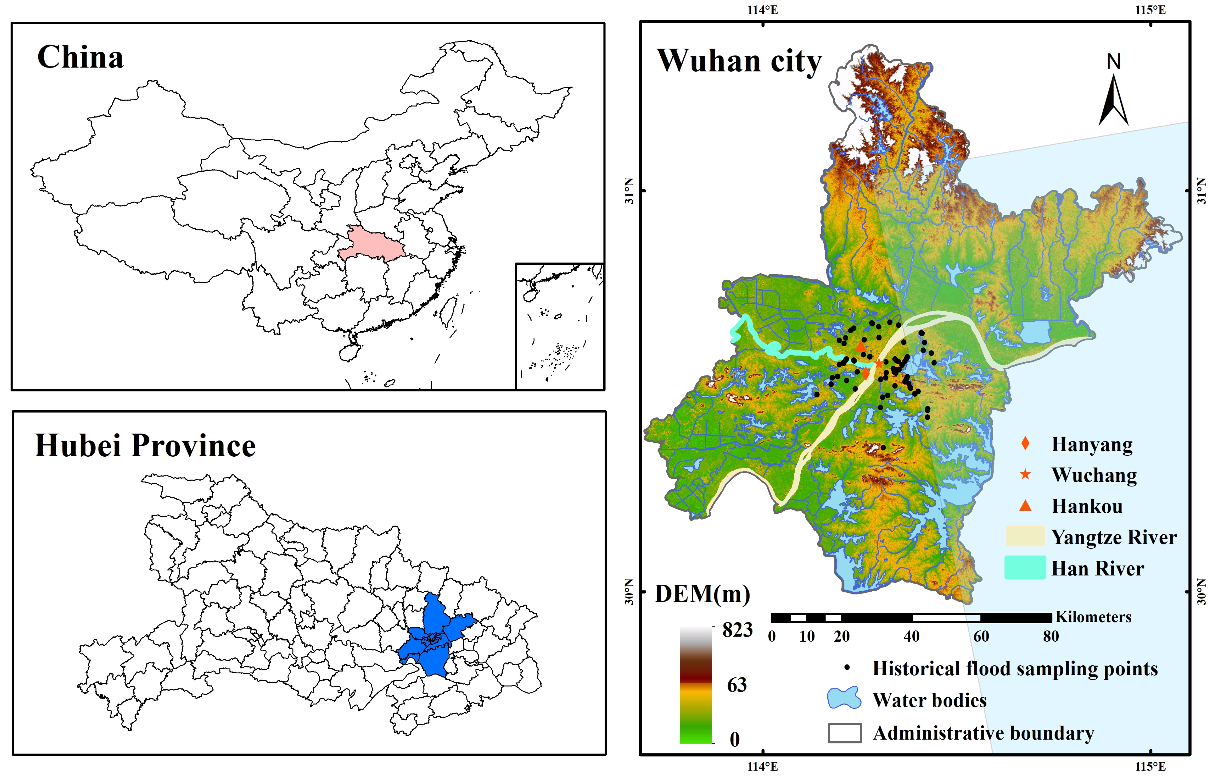
Figure 1. Location of Wuhan City and the historical flood sampling points in the city. The pink area in the upper left image is Hubei Province; The blue area in the picture below is Wuhan City. The semitransparent blue area in the right image represents the coverage range of Sentinel-1 images used in this experiment.
Remotesensing 15 03601 g001
Figure 2. Flowchart for expanding the flood inventory data and predicting flood susceptibility using the expanded FID and machine learning models.
Remotesensing 15 03601 g002
Figure 3. The spatial distribution of the historical and expanded FPs and the comparison of the extracted flood area with previous studies. (a) Historical and expanded flood and non-flood sampling points used for training and validating the models. The Flood points_b means the historical FPs; the Flood points_a means the expanded FPs. (b) Flood and non-flood points used for testing the models. In addition, the blue semi-transparent area is the Sentinel-1 image area used in this study. (c) Flood areas (red color) extracted by Zeng et al. (2020) [22] near Wu Lake (Adapted with permission from Ref. [22]. 2020, Ziyue Zeng). Its specific location is in the red box in (a). (d) Flood areas (red color) extracted in this study for comparing with results of Zeng et al. (2020) [22]. The Water 1 represents the water surface data from the National Catalogue Service for Geographic Information (see Section 2.2); the Water 2 is the water surface extracted in this study. (e) Locations of the FPs identified based on the flood areas extracted by Zeng et al. (2020) [22] in (c).
Remotesensing 15 03601 g003
Figure 4. Spatial distribution of the flood conditioning factors in Wuhan City.
Remotesensing 15 03601 g004
Figure 5. The ROC curves and corresponding AUC values of the machine learning models in the testing period. The symbol “_b” means the AUC of the machine learning models without considering the expanded FID, while the symbol “_a” means the AUC of the machine learning models considered the expanded FID.
Remotesensing 15 03601 g005
Figure 6. Flood susceptibility maps of Wuhan City based on the SVM, RF and ANN models. The symbols “_a” and “_b” mean considering and not considering the expanded FID for the corresponding models, respectively. The small block diagrams show the details of the flood susceptibility map in the red box region.
Remotesensing 15 03601 g006
Figure 7. Area and area proportion of the flood susceptibility classification (km2). (a,c) using scenario 2 data modeling, while (b,d) using scenario 1 data modeling with *.
Remotesensing 15 03601 g007
Figure 8. The variability map generated by the flood susceptibility map in Figure 7 as well as some important conditioning factors. Among them, (ad) represent the variability map generated by the flood susceptibility map of (ad) in Figure 7, and (eh) show the details of the red box area of (ad). (il) represent four important conditioning factors, namely elevation, distance to water, NDVI, and distance type, in the (eh) regions. In addition, the classification of the distance type is shown in Table 3.
Remotesensing 15 03601 g008
Table 1. Flood conditioning factors used in this study for driving the machine learning models.
Flood Conditioning FactorData SourceMeaningResolutionEquationVariable Description
ElevationGDEM V2The distance from a point along the vertical line to the absolute base plane30 MExtraction based on DEM-
SlopeGDEM V2Degree of surface steepness30 MExtraction based on DEM-
AspectGDEM V2Direction of projection of the slope normal on the horizontal plane30 MExtraction based on DEM-
CurvatureGDEM V2The degree of curvature of a curve at a point30 MExtraction based on DEM-
NDVILandsat-8 OLI_TIRSNormalized difference vegetation index30 M NDVI = NIR     R NIR   +   R where NIR and R refer to the top of the atmosphere reflectance of the near-infrared (0.86 µm) and red band, respectively.
NDBILandsat-8 OLI_TIRSNormalized differences built-up index30 M NDBI = SWIR     NIR SWIR   +   NIR where SWIR and NIR are the top of the atmosphere reflectance of the shortwave infrared (2.2 µm) and near infrared band, respectively.
TWIGDEM V2Topographic wetness index30 M TWI = ln A S / tan β where AS is the specific catchment area in units of (m2 m−1) and β is a slope in radians [36].
SPIGDEM V2Stream power index 30 M SPI = A S · tan β
Soil typeNational 1:6 million soil-type datasetSoil classification1:600 million--
Land useFROM-GLC 10 2017v1Land use classification10 M--
Distance to water1:1 million basic geographic vector map dataThe Euclidean distance to the closest water area1:100 million--
Distance type1:1 million basic geographic vector map dataClassification of water body types nearest to pixels based on the Euclidean distance1:100 million--
Table 2. Spatial distribution of the flood conditioning factors in Wuhan City.
Land UseSoil TypeDistance Type
CodeDescriptionCodeDescriptionCodeDescription
0-ASwampy SoilIYangtze and Han Rivers
1CropBLakes and waterIIRivers
2ForestCDark yellow–brown loamIIILakes
3GrassDAlluvial soilsIVReservoirs
4ShrubETidal soils--
5WetlandFRice soils--
6WaterGYellow–brown loam--
7TundraHYellow–brown loam--
8ImperviousIYellow–red loam--
9Bare landJYellow–brown loam--
10Snow/iceKPercolating rice--
11CloudLTrapped rice--
--MRed loam--
--NGrey tide soil--
--ORed loamy soils--
--PBrown–red loam--
--QDe-submerged rice--
--RUrban area--
--SRiver and stream--
--TRinsed rice--
Table 3. The VIF analysis of the selected flood conditioning factors.
FactorsVIFFactorsVIF
Elevation3.81Slope4.58
NDVI5.25Curvature1.12
SPI1.43NDBI2.85
TWI5.82Distance to water2.91
LU2.84Distance type11.83
Aspect3.53Soil type9.50
Table 4. Adjustment of the model hyperparameters for the ANN, RF, GBDT, KNN and SVM models in Wuhan City.
ModelHyperparameters of without Considering Data ExpansionHyperparameters of with Considering Data Expansion
RFn_estimators = 15n_estimators = 25
GBDTn_estimators = 100, loss = ‘deviance’, learning_rate = 0.1n_estimators = 100, loss = ‘deviance’, learning_rate = 0.1
ANNbatch_size = 4, epoch = 60, activation function: ReLUbatch_size = 4, epoch = 80, activation function: ReLU
KNNn_jobs = −1, n_neighbors = 7n_jobs = −1, n_neighbors = 15
SVMkernel = ‘rbf’, C = 195, gamma = 1.0, probability = Truekernel = ‘rbf’, C = 198, gamma = 1.0, probability = True
Table 5. The AUC values of the machine learning models used in this study in the model validation phase.
Model in Scenario 1, without Considering Expanded FIDAUC Value under Cross-ValidationAUC Value under Spatial Cross-ValidationModel in Scenario 2, with Considering Expanded FIDAUC Value under Cross-ValidationAUC Value under Spatial Cross-Validation
RF0.890.97RF0.900.95
GBDT0.900.98GBDT0.920.95
KNN0.830.82KNN0.890.81
SVM0.870.82SVM0.920.86
ANN0.970.92ANN0.940.89
Table 6. The results of the performance metrics used to evaluate the performances of the machine learning models during the testing phase.
ScenarioModel KappaAUCPrecisionRecallF1-ScoreImprovement of AUC (%)
Models in Scenario 1RF0.250.800.670.620.59-
GBDT0.300.760.640.60.58-
KNN0.470.770.750.730.72-
SVM0.570.880.750.740.73-
ANN0.600.830.810.790.8-
Models in Scenario 2RF0.720.930.860.860.8616.25
GBDT0.700.910.850.850.8519.74
KNN0.530.860.830.830.8311.69
SVM0.700.890.770.760.761.14
ANN0.720.910.830.910.869.64
Disclaimer/Publisher’s Note: The statements, opinions and data contained in all publications are solely those of the individual author(s) and contributor(s) and not of MDPI and/or the editor(s). MDPI and/or the editor(s) disclaim responsibility for any injury to people or property resulting from any ideas, methods, instructions or products referred to in the content.